Impacts of climate change on flow composition using a model tailored to runoff components

Full text

(1)IMPACTS OF CLIMATE CHANGE ON FLOW COMPOSITION USING A MODEL TAILORED TO RUNOFF COMPONENTS. W.J. Schreur March 2019.

(2)

(3) Title. Author. Institute. Supervisors. Impacts of climate change on flow composition using a model tailored to runoff components. Wouter Jan Schreur. University of Twente Institute of Geophysics, Polish Academy of Sciences. Dr. ir. M.J. Booij University of Twente, Department of Water Engineering and Management Dr. M.S. Krol University of Twente, Department of Water Engineering and Management. Advisor. Date. Prof. dr. hab. eng. R.J. Romanowicz Institute of Geophysics, Polish Academy of Sciences; Department of Hydrology and Hydrodynamics. 12 March 2019.

(4) Summary Over the past decades various studies have indicated that climate change and its accompanying hydrological impacts are a prevalent issue. Without proper measures the impact of floods and droughts can extend to various water dependent sectors including agriculture, forestry, fishing, hydropower and tourism. Generally, climate change impact on river discharge is assessed based on projected changes to the total runoff. It is however argued that looking exclusively at the total river discharge is not a sufficient indicator and additional insights in the runoff would be a step towards improvements on runoff modelling and gaining insight in climate change impacts. The goal of this research is to gain insight in the runoff components that together make up the total runoff and how to calibrate a hydrological model such that the skill at which the individual runoff components are simulated improves. These new insights will then be applied to calibrate a hydrological model tailored towards simulating runoff components and assess the impacts of climate change not only on the total runoff but also the impact it has on the runoff components and the composition of the total runoff. For this research, hydrological modelling will be done using the Hydrologiska Byråns Vattenbalansavdelning (HBV) model. Three Polish catchments: Biala Tarnowska, Dunajec and Narewka catchments are used as test cases in this research. To find if there is a relationship between the criteria that are used in model calibration and the skill at which the HBV model simulates the runoff components two objective functions have been used for model calibration. The two criteria or objective functions that are used for model calibration are the Nash-Sutcliffe efficiency criterion (NS) that emphasised high flows and the logarithmically transformed Nash-Sutcliffe (NSL) which emphasises baseflow. The two objective functions are used in a weighted manner by assigning a weight to each function to be able to later identify a trade-off between the objective functions. The weights assigned to both objective functions are varied between 0% to 100% at increments of 10% while keeping the sum of the weights equal to 100%. Calibration was done using the SCEM-UA calibration algorithm which resulted in 11 unique parameter sets for each catchment, each corresponding to a combination of NS and NSL function weights. The contributions of the runoff components are derived from the total runoff using the Wittenberg baseflow filter (Wittenberg, 1999). The skill at which the runoff components are simulated is assessed by using the NS as performance indicator and comparing the individual runoff components derived from simulations to those derived from the observations. Correlation between the skill at which runoff components are simulated and the NSL weight used in model calibration indicates that, for all three catchments, there is a significant correlation between the NSL weight and the HBV model its ability to skilfully simulate the baseflow component. A significant correlation between the NSL weight used in calibration and the skill at which the HBV model simulates the fast runoff component was only found for the Narewka catchment. Because the goal is to improve on the skill at which runoff components are simulated, the final calibration has been done using exclusively the NSL as performance indicator for model calibration. Using the HBV model that is calibrated for the three catchments using the NSL as performance indicator, climate change impacts on the total runoff have been assessed and additionally the impact that climate change has on the runoff components and the composition of the runoff are assessed. For climate change (re)assessment synthetic climate data is used from the EURO-CORDEX initiative. The datasets consist of precipitation and temperature simulations generated by seven combinations of General Circulation Models (GCM) and Regional Climate Models (RCM).

(5) Assessment of climate change impacts on projected flow resulted in findings that correspond to earlier modelling studies that have used the considered catchments as case studies (Osuch et al., 2016; Piniewski, 2017). The annual total runoff is projected to increase with the largest projected increase observed in the winter (December, January and February) and spring (March, April and May) periods. Separation of the runoff in the fast runoff component and the baseflow component indicated that there are differences in the composition of the total runoff between the three catchments for the observational period. When projected flows are assessed differences between the catchment are still present but differences between the simulations that are done using the GCM/RCM combinations are also present. These differences between the seven GCM/RCM combinations appeared to be consistent between the catchments and are assumed to be related to the individual GCM and/or RCM models that are used in simulating the climate data. Looking at the impact that projected climate change will have on the composition of the runoff indicated that the composition of the total runoff is not projected to change in the future for either of the climate models. Previously, climate change projections have shown that the intensity of precipitation evens is projected to increase which results in the expectations that more fast runoff will occur. Findings from this research however do not support this expectation. This might be caused by not taking into account changes that the catchments themselves may undergo over the upcoming decades. Wang & Cai (2010) have shown that the main driving force in changes in the flow composition is human interference (e.g. urbanisation or canalisation), an aspect that is not taken into account in this study. Another explanation for the absence of these changes can be found in the climate data that has been used in this research. Simulations from the GCM or downscaling to a RCM could have resulted in climate data that does not contain this increase in intensity but rather display a gradual uptrend in the precipitation. These possible causes however were outside of the scope of this research and have not been further pursued. In conclusion, there appears to be a significant relationship between objective functions that are used in model calibration and the skill at which runoff components can be simulated. This again shows the importance of selecting the most suited objective functions according to the research objective. But even while new insights have been gained in this area it displays that the impacts of climate change on river runoff might be restricted to changes in the total runoff after all. And that the composition of the runoff is not projected to change when compared to runoff simulations of the present situation. To conclude this research, several recommendations have been made that might be a worthwhile endeavour to pursue in order to be able to make these results more applicable wider variety of cases and to further improve on modelling runoff components..

(6) Table of Contents 1. 2. Introduction ..........................................................................................................................................................5 1.1. Background and Relevance ..........................................................................................................................5. 1.2. Problem Description ....................................................................................................................................6. 1.3. Research objective .......................................................................................................................................6. 1.4. Research Strategy and Reading Guide .........................................................................................................7. Study area and data sets .......................................................................................................................................9 2.1 2.1.1. Biała Tarnowska .....................................................................................................................................10. 2.1.2. Dunajec ..................................................................................................................................................10. 2.1.3. Narewka .................................................................................................................................................10. 2.2. Discharge ...............................................................................................................................................11. 2.2.2. Precipitation...........................................................................................................................................12. 2.2.3. Temperature ..........................................................................................................................................13 Climate change data sets ...........................................................................................................................14. Methodology.......................................................................................................................................................17 3.1. Hydrological model ....................................................................................................................................17. 3.1.1. Model choice .........................................................................................................................................17. 3.1.2. Model description and model equations ...............................................................................................18. 3.2. Sensitivity analysis......................................................................................................................................21. 3.2.1. Objective functions ................................................................................................................................21. 3.2.2. Sobol’s method ......................................................................................................................................22. 3.3. Model calibration .......................................................................................................................................24. 3.3.1. Calibration algorithm choice ..................................................................................................................24. 3.3.2. Calibration algorithm .............................................................................................................................24. 3.3.3. Calibration and validation period ..........................................................................................................25. 3.4. Simulation of runoff components ..............................................................................................................25. 3.4.1. Hydrograph separation ..........................................................................................................................25. 3.4.2. Simulation of runoff components ..........................................................................................................26. 3.5 4. Observational data sets..............................................................................................................................11. 2.2.1. 2.3 3. Catchments ..................................................................................................................................................9. Climate change impact ...............................................................................................................................27. Results .................................................................................................................................................................29 4.1. Sensitivity Analysis .....................................................................................................................................29. 1.

(7) 4.2. Model calibration .......................................................................................................................................31. 4.2.1. Parameter ranges ..................................................................................................................................31. 4.2.2. Calibration Results .................................................................................................................................33. 4.3. Simulation of runoff components ..............................................................................................................36. 4.4. Trade-off between objective functions ......................................................................................................37. 4.5. Climate change impact ...............................................................................................................................38. 5. 4.5.1. Model performance on reference period ..............................................................................................38. 4.5.2. Climate change impact on the total runoff ............................................................................................40. 4.5.3. Climate change impact on the runoff components ...............................................................................41. 4.5.4. Projected changes in low flows .............................................................................................................44. Discussion ...........................................................................................................................................................47 5.1. Datasets .....................................................................................................................................................47. 5.2. Model calibration .......................................................................................................................................47. 5.3. Results ........................................................................................................................................................48. 6. Conclusion ...........................................................................................................................................................51. 7. Recommendations ..............................................................................................................................................52. 8. References ..........................................................................................................................................................53. 9. Appendices..........................................................................................................................................................59 A.. Appendix A .....................................................................................................................................................59. B.. Appendix B......................................................................................................................................................62. C.. Appendix C......................................................................................................................................................63. D.. Appendix D .....................................................................................................................................................66. 2.

(8) List of Figures Figure 2-1: Geographical locations of the considered catchments. (Romanowicz et al., 2016)....................................9 Figure 2-2: Daily mean discharges for the Biała Tarnowska, Dunajec and Narewka catchments for the 1971-2010 period ..........................................................................................................................................................................11 Figure 2-3: Mean monthly precipitation values for the observation period 1971-2010 .............................................12 Figure 2-4: Observed mean daily temperature for the 1971-2010 period ..................................................................13 Figure 2-5: Annual sum precipitation for the Biała Tarnowska, Dunajec and Narewka catchments for the 1971-2100 period from the seven GCM/RCM combinations ........................................................................................................14 Figure 2-6: Annual mean temperature for the Biała Tarnowska, Dunajec and Narewka catchments for the 1971-2100 period from the seven GCM/RCM combinations ........................................................................................................15 Figure 3-1: HBV model structure, adopted from Knoben (2013) ................................................................................18 Figure 3-2: Visual representation of the temperature interval and temperature threshold (Knoben, 2013) .............19 Figure 3-3: Wittenberg's baseflow separation applied to the Biala TArnowska catchment for the year 1976...........26 Figure 4-1: Results of variance decomposition for the Biała Tarnowska catchment ..................................................30 Figure 4-2: Results of variance decomposition for the Dunajec catchment ................................................................30 Figure 4-3: Results of variance decomposition for the Narewka catchment ..............................................................30 Figure 4-4: Calibration results for the Biała Tarnowska catchment ............................................................................33 Figure 4-5: Calibration results for the Dunajec catchment..........................................................................................34 Figure 4-6: : Calibration results for the Narewka catchment ......................................................................................35 Figure 4-7: NS Scores for the fast runoff and baseflow components for the Biała Tarnowska catchment .................36 Figure 4-8: NS scores for the fast runoff and baseflow components for the Dunajec catchment ..............................36 Figure 4-9: NS scores for the fast runoff and baseflow components for the Narewka catchment .............................37 Figure 4-10: Modelled Annual mean flow from the Biała Tarnowska, Dunajec and Narewka catchments for the 19712100 period .................................................................................................................................................................41. 3.

(9) List of Tables Table 2-1: Observed mean flow and standard deviation for the years 1971-2010 .....................................................12 Table 2-2: Minimum, mean and maximum observed yearly precipitation for the Biała Tarnowska, Dunajec and Narewka catchments ...................................................................................................................................................13 Table 2-3: List of GCM/RCM combinations used in this study ....................................................................................14 Table 3-1: SCEM-UA algorithm parameters (Vrugt et al., 2003b) ...............................................................................25 Table 4-1: HBV model parameters that will be taken into account for model calibration per catchment .................31 Table 4-2: Definitive parameter ranges used in calibration of the HBV model for the Biała Tarnowska catchment ..31 Table 4-3: Definitive parameter ranges used in calibration of the HBV model for the Dunajec catchment ...............32 Table 4-4: Definitive parameter ranges used in calibration of the HBV model for the Narewka catchment ..............32 Table 4-5: Default parameter values for the HBV model (SMHI, 2006) ......................................................................32 Table 4-6: Correlations between the NS scores of the components and the weight assigned to the NSL .................37 Table 4-7: Mean runoff from the Biała Tarnowska catchment per GCM/RCM combination and deviation from the observated mean runoff ..............................................................................................................................................39 Table 4-8: Mean runoff from the Dunajec catchment per GCM/RCM combinations and deviation from the observed mean runoff .................................................................................................................................................................39 Table 4-9: Mean runoff from the Narewka catchment per GCM/RCM combinations and deviation from the observed mean runoff .................................................................................................................................................................39 Table 4-10: changes in percentage per year in modelled annual runoff over the 1971-2100 period for the Biała Tarnowska, Dunajec and Narewka catchments...........................................................................................................41 Table 4-11: Derived BFI for the Biała Tarnowska catchment from runoff simulations for each of the seven GCM/RCM combinations for the reference, near-future and far-future period ...........................................................................42 Table 4-12: Derived BFI for the Dunajec catchment from runoff simulations for each of the seven GCM/RCM combinations for the reference, near-future and far-future period ...........................................................................42 Table 4-13: Derived BFI for the Narewka catchment from runoff simulations for each of the seven GCM/RCM combinations for the reference, near-future and far-future period ...........................................................................42 Table 4-14: Seasonal BFI contributions to the total fow for the Biała TArnowska catchment for the reference, nearfuture and far-future periods ......................................................................................................................................43 Table 4-15: Seasonal BFI contributions to the total fow for the Dunajec catchment for the reference, near-future and far-future periods ........................................................................................................................................................43 Table 4-16: Seasonal BFI contributions to the total fow for the Narewka catchment for the reference, near-future and far-future periods .................................................................................................................................................43 Table 4-17: Q90 for the Biała Tarnowska, Dunajec and Narewka catchments derived from the observed runoff for the reference period ....................................................................................................................................................44 Table 4-18: Mean Q90 for the Biała Tarnowska, Dunajec and Narewka catchments derived from the simulated runoff for the reference, near-future and far-future period ..................................................................................................44. 4.

(10) 1 INTRODUCTION This chapter of the report will be used to introduce the topic of this research and will set the scope of what this research will consist of. In section 1.1 background information on the topic will be discussed and the relevance of this research will be pointed out. The problem description is presented in section 1.2 along with the research questions that have been defined in section 1.3. An overview of how the report will be structured is presented in section 1.4.. 1.1 BACKGROUND AND RELEVANCE From studies and observations it has become more and more apparent that climate change and its hydrological impacts are a prevalent issue. Without proper measures the impact of floods and droughts extend to various water dependent sectors, including agriculture, forestry, fishing, hydropower and tourism. (Demirel et al., 2013) Additionally extreme events can have direct societal impacts by disrupting e.g. domestic water supply and infrastructure. Therefore, it is important to gain more insight in the occurrence of hydrologically extreme events and projected changes in their magnitude and probability of occurrence (CHIHE, 2016). In the Intergovernmental Panel on Climate Change’s Assessment Report 5 it is described that, over mid-latitude regions, it is very likely that extreme precipitation events will become more frequent and also become more intense (Pachauri & Meyer, 2014) which leads to an increased risk of urban- and flash flooding caused by rainfall. In addition to this, projections also show a shorter snow season in mountainous areas which means that less snow will accumulate which leads to a decreased risk of spring floods (WHO, JRC, & EEA, 2008). Translation of climatic variables and catchment characteristics to river discharge is done using hydrological models. Many studies have been done into the functioning of these models as well as the application of the models on case studies. In the majority of the case studies where hydrological models are applied to model runoff from catchments the focus has been on the total runoff (e.g. Lindström et al., 1997; Beven, 2012). Also, for assessment of the impacts of climate change the effects are generally assessed based on changes to the projected total runoff (e.g. Bisterbosch, 2010; Osuch et al., 2016). For various Polish catchments for example, studies on climate change impact have shown that projected changes will lead to a shift in the timing of runoff and change in the magnitude of runoff peaks. The flood season is expected to shift from March-April to January-February due to the earlier snowmelt (Romanowicz et al., 2016). The total runoff can also be seen as the combined sum of the runoff components, a faster, direct runoff component and, a slower, baseflow component. These individual components often go unobserved as generally only the total runoff is measured and the origins of the runoff remain unknown. Retracing the origin of the baseflow can be done by tracer analysis if the data is present in addition to the observations of the runoff. Alternatively, the baseflow can be derived from the total runoff by making use of filtering techniques. These filtering techniques can be based on different measurable aspects of the hydrograph but are most commonly based on the recession parameter that is derived from the receding part of the hydrograph. Studies into the impact of climate change on the total runoff are common and widespread but studies into runoff components and the composition of the total runoff are far more uncommon. For proper functioning of a hydrological model it is paramount that the correct parameter values are found for the hydrological model by calibrating them. In model calibration one or more objective functions can be used to assess the model performance by comparing the model output to observations. Different objective functions emphasise different parts of the hydrograph during the model calibration and the correct objective function should be determined a-priori according to the goal of the research (Chang, 2014). Often a single objective function is used in. 5.

(11) model calibration (e.g. Knoben, 2013; Osuch et al., 2016; Romanowicz et al., 2016) but there are also various reported cases where a combination of objective functions was used in model calibration (e.g. Dawdy et al., 1971; Li et al., 2014; Lv et al., 2018). Model calibration using multiple objective functions in e.g. the aforementioned studies was done by assigning static weights to the objective functions which were arbitrarily assigned. Because of the static weights that were assigned to the different objective functions it is uncertain if the weighting of the functions has resulted in the best parameterisation of the model of the research purpose.. 1.2 PROBLEM DESCRIPTION Assessing impacts of climate change by looking at the total river discharge does not give full insight in the alterations the river discharge might undergo. Even looking at more specific parts of the hydrograph, e.g. the maximum, mean or seasonal flows does not show the full picture of the hydrological impact of climate change on river runoff. A more thorough way to assess the changes a river system undergoes is to decompose the runoff into its components that together make up the total runoff and look at the impact that climate change has on the individual components and the composition of the total runoff. Because the individual components of the runoff are usually not observed (Romanowicz, 2017), calibration and validation of hydrological models is therefore done based on the hydrograph representing the total runoff. This might lead to a model calibration that and performs best for simulating the total runoff but might not correctly describe the individual runoff components. The underlying problem herein is that little research has been done into a calibration method that can be applied such that the model output not only corresponds to the observed total runoff but that also the derived runoff components are simulated correctly. It is known that different objective functions emphasize different parts of the hydrograph and objective functions can be chosen according to the goal of the research. However, the impact that different objective functions have on the model its ability to simulate the individual runoff components is a topic in which little research has been done. This limitation leads to the uncertainty on the reliability of more detailed analysis on the effect of changing climatological conditions not only on the projected total runoff but also on the runoff components and the composition of the runoff.. 1.3 RESEARCH OBJECTIVE The goal of this research is to find whether there is a relationship between the objective functions that are used during model calibration and the ability of a hydrological model to correctly simulate runoff components in addition to correctly simulating the total runoff. This potential relationship will then be used to calibrate a hydrological model that is tailored towards simulation of runoff components. With this calibrated model, the impact of climate change will be assessed for a test case considering three Polish catchments. The impact of climate change will be evaluated by assessing the impact that projected climate change has on the composition of the runoff in addition to the impact it has on the total runoff. To reach these objectives and guide the research the following research questions have been formulated: 1. 2. 3. 4.. What is the trade-off between objective functions for model calibration for the accuracy at which runoff components are simulated? Which parameter set allows the HBV model to correctly simulate both the total runoff and the runoff components for the Biała Tarnowska, Dunajec and Narewka catchments? What are the contributions of the runoff components to the observed runoff for the Biała Tarnowska, Dunajec and Narewka catchments? What are the impacts of projected climate change on the runoff components and the composition of the runoff? 6.

(12) 1.4 RESEARCH STRATEGY AND READING GUIDE To answer the aforementioned research questions and achieve the objective of this research the research and report are structured as follows. Firstly, the HBV model will be set up with a reduced number of parameters. The parameters which will be involved in the model calibration are determined per catchment by executing a sensitivity analysis. The model will be calibrated for various combinations of weights assigned to the Nash-Sutcliffe and the logarithmic NashSutcliffe objective functions. Multiple calibrations for various objective function weights allow for a comparison between the scores achieved on the objective functions and the weights assigned to the objective functions. From this comparison insight will be gained in the trade-off between the objective functions and the model its ability to correctly simulate the runoff components. Based on the trade-off between the objective functions the most appropriate weights that will be assigned to the individual objective functions will be determined in order to allow for the most accurate simulation of the individual runoff components. With the model being correctly set up and calibrated the impact of climate change can be assessed. The impacts of climate change will firstly be evaluated on the total runoff before going into a more detailed analysis of the impact that climate change is projected to have on the runoff components. Assessing the impact of climate change will be done by comparing the projected changes for the near-future (2021-2050) and far-future (2071-2100) to the reference period (1976-2005). Climate change impact on the runoff components will be evaluated by looking more closely at the composition of the total runoff. The total runoff will be separated into the baseflow components and the quick runoff component. The contribution of the two individual components to the runoff will be used to indicate whether climate change will impact the composition of projected flows for the near-future and far-future relative to the composition of the flow in the reference period. The Biała Tarnowska, Dunajec and Narewka catchments that are considered in this research as well as the datasets what will be used will be presented in chapter 2. In chapter 3, the aforementioned approach to the research will be discussed in more detail. The results that are obtained will be presented in chapter 4 and discussed in chapter 5 with the final conclusions and recommendations being presented in chapters 6 and 7.. 7.

(13) 8.

(14) 2 STUDY AREA AND DATA SETS In this chapter of the report the data sets that will be used in this study will be presented. In chapter 2.1 the catchments that will be used in the case study are presented along with a description of the characteristics of the catchments. Chapter 2.2 will be used to describe the datasets containing the observational data and in chapter 2.3 the datasets containing the climate projections will be presented.. 2.1 CATCHMENTS In the case study that will be executed in this research three Polish catchments will be considered. The three catchments that are chosen for this purpose are the Biała Tarnowska, the Dunajec and the Narewka catchments. In the following sections these catchments will be individually described and characterized. The choice for these specific catchments has been made based on previous research. The Polish-Norwegian project Climate Change Impact on Hydrological Extremes (CHIHE) has identified catchments that were suited for rainfall runoff and climate change modelling. Romanowicz et al. (2016) describes the selection procedure that was used to identify these catchments. In this study, ten nearly-natural Polish catchments were identified and flood regimes have been attributed to each catchment. In earlier modelling studies from the CHIHE project for these catchments, rainfall runoff modelling has been done by using the HBV model. The accuracy at which their calibrated models were able to reproduce the observed river runoff has been used as criteria for catchment selection in this study. Both the calibration and validation periods are taken into account in this consideration. This choice should ensure that catchments with the best data quality will be used. In Figure 2-1 a map is displayed where the geographical location of the catchments can be found along with the flood regime attributed to each catchment.. FIGURE 2-1: GEOGRAPHICAL LOCATIONS OF THE CONSIDERED CATCHMENTS. (ROMANOWICZ ET AL., 2016). 9.

(15) 2.1.1 BIAŁA TARNOWSKA The Biała Tarnowska catchment is located in the southern regions of Poland in the Carpathian Mountains and extends north from the Polish-Slovakian border. The source of the river has an elevation of 730 m above mean sea level and the total length of the Biała Tarnowska is 101.8 km along which the river banks are unregulated and in a natural state. The catchment area of the Biała Tarnowska that is drained by the river is 956.9 km 2 and is in a nearlynatural state (Napiorkowski et al., 2014). The southern, mountainous, region of the catchment representing about 25% of the catchment area is covered with woodland and has relatively steep river slopes which are in the range of 10‰. The northern regions of the catchment can be described as deep river valleys where fields, meadows and pastures predominate. In this area of the catchment the river slope is much gentler in the range of 0.9 – 5 ‰. Biała Tarnowska is a perennial river that is characterized by its mixed runoff regime that contains elements of both snowmelt and rainfall as driving mechanisms for runoff generation (Romanowicz et al.,2016). T. 2.1.2 DUNAJEC The Dunajec catchment is situated in southern Poland in the Tarta Mountains and is formed at the confluence of the Czarny Dunajec (Black Dunajec) and the Biały Dunajec (White Dunajec). The Dunajec River has a length of 274 km of which 27 km forms a natural border between Slovakia and Poland. The drainage area of the Dunajec basin that discharges to the Dunajec River is 681.1 km2 of which nearly 60% is used for agricultural purposes. The Dunajec is a nearly natural the river with unregulated banks that are in a natural state and an average slope of the Dunajec is 8‰ (Rowinsky, 2013; Kundewicz et al., 2016). Romanowicz et al. (2016) classified the runoff regime of the Dunajec River as a predominantly rainfall fed river.. 2.1.3 NAREWKA The Narewka Catchment is located in the north-eastern regions of Poland on the Polish Plain and extends over the border with Belarus. The area of the catchment is 635.3 km2 of which the largest part is on Polish territory. The Narewka river that is fed from this catchment has a length of 61.1 km of which approximately 22 km in Belarus with the slope of the river ranging between 0.35‰ and 0.64‰ (Jedrzejewska & Jedrzejewski, 1998). In Romanowicz et al. (2016) the Narewka catchment was classified as a nearly-natural catchment with a flood regime that is predominantly fed by snowmelt. Nearly the entire catchment (88%) is covered with forests. Of the remaining area 11% is used for agriculture.. 10.

(16) 2.2 OBSERVATIONAL DATA SETS The observational datasets that are used for this study contain observations on the river discharge and climatological variables for the selected catchments. The datasets contain observations covering the period from 1971 until the 2010 measured at daily intervals. The datasets have been checked on data quality i.e. the datasets contain no obvious outliers and/or missing values. In the following sections the available datasets will individually be described briefly and presented in figures.. 2.2.1 DISCHARGE Discharge data as provided by the Institute of Geophysics Poland (IGF PAN) is the observed river discharge at the gauging station at the outlet of the catchment. The river discharge is determined based on water level measurements which have been converted using rating curves. In Figure 2-2 the mean daily observed discharge for each of the three catchments are presented. Peaks in the discharge can be observed mainly in the spring and summer periods. These spring floods are largely the result of snowmelt whereas discharge peaks in the summer are caused by precipitation events. Mean flow and standard deviation for the catchments are presented in Table 2-1Error! Reference source not found... FIGURE 2-2: DAILY MEAN DISCHARGES FOR THE BIAŁA TARNOWSKA, DUNAJEC AND NAREWKA CATCHMENTS FOR THE 1971-2010 PERIOD. 11.

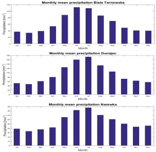
(17) TABLE 2-1: OBSERVED MEAN FLOW AND STANDARD DEVIATION FOR THE YEARS 1971-2010. Catchment Biała Tarnowska Dunajec Narewka. Mean flow [m3 s-1] 9.5 14.6 3.1. Standard deviation [m3 s-1] 20.3 17.1 3.5. 2.2.2 PRECIPITATION Precipitation data for the catchments is taken from one or a combination of multiple meteorological observation stations located in or close to the catchment. The Narewka catchment is the only catchment that makes use of observations from only one measurement station. The data sets of the Biała Tarnowska and Dunajec make use of data derived from 5 and 3 measurement stations respectively. The areal average precipitations that is used in this study is derived from the observations from the individual meteorological stations and averaged to one representative value for the entire catchment by using Thiessen polygons (Benninga et al., 2017). Precipitation values are provided in mm at daily measurement intervals. In Figure 2-3 the average monthly precipitation over the observation period is presented to show how the precipitation is distributed over the year. It can be seen that the Biała Tarnowska and Dunajec catchments where the flood regime is dominated by rainfall or is a mixed regime the summer precipitation is relatively much higher than in the snowmelt dominated Narewka catchment. Annual minimum, mean and maximum observed values for the precipitation over the 1971-2010 period are presented in Table 2-2.. FIGURE 2-3: MEAN MONTHLY PRECIPITATION VALUES FOR THE OBSERVATION PERIOD 1971-2010. 12.

(18) TABLE 2-2: MINIMUM, MEAN AND MAXIMUM OBSERVED YEARLY PRECIPITATION FOR THE BIAŁA TARNOWSKA, DUNAJEC AND NAREWKA CATCHMENTS. Catchment Biała Tarnowska Dunajec Narewka. Minimum observed precipitation [mm] 552 816 448. Average observed precipitation [mm] 752 1 120 651.1. Maximum observed precipitation [mm] 1 073 1 460 933. 2.2.3 TEMPERATURE From the same measurement stations that are used for the precipitation observations the temperature observations are obtained for the three catchments. In Figure 2-4 the mean daily observed temperature for the 1971-2010 period is displayed in degrees Celsius. The temperature observations are used in calculating the potential evapotranspiration according to the method of Hamon (Hamon, 1961) and as model inputs for the snow accumulation and snowmelt routines of the hydrological model.. FIGURE 2-4: OBSERVED MEAN DAILY TEMPERATURE FOR THE 1971-2010 PERIOD. 13.

(19) 2.3 CLIMATE CHANGE DATA SETS The datasets containing the future climate projections contain the results from several climate model simulations. The climate projection data used in this research consists of the daily temperature and precipitation and were obtained from the EURO-CORDEX initiative (http://www.euro-cordex.net/). The climate change scenario that these projections represent is the RCP 4.5 scenario which is described in the Fifth Assessment Report (AR5) by the Intergovernmental Panel on Climate Change (IPCC, 2013). All climate simulations are done using a General Circulation Model (GCM) and a Regional Climate Model (RCM). In total seven GCM/RCM combinations are used to generate the dataset resulting in an ensemble of seven different projections. The seven GCM/RCM combinations that are used to generate the climate change projections are presented in Table 2-3 along with the affiliated institute (Meresa & Romanowicz, 2017). TABLE 2-3: LIST OF GCM/RCM COMBINATIONS USED IN THIS STUDY. 1 2 3 4 5 6 7. GCM EC-EARTH EC-EARTH EC-EARTH EC-EARTH MPI-ESM-LR MPI-ESM-LR CNRM-CM5. RCM RCA-4 HIRHAM5 CCLM-4-8-17 RACMO22E CCLM-4-8-17 RCA4 CCLM4-8-17. Institute Swedish Meteorological and Hydrological Institute Danish Meteorological Institute NCAR UCAR Danish Meteorological Institute Max Planck Institute for Meteorology Max Planck Institute for Meteorology CARFACS, France. In Figure 2-5 the projected annual precipitation from the seven GCM/RCM models is presented for the 1971-2100 period for the three catchments considered in this study. Each coloured dot represents a GCM/RCM combination and the black line represents the ensemble mean annual precipitation of the seven GCM/RCM combinations. All three catchments show an upward trend in the mean annual precipitation with the strongest upward trend for the Narewka catchment.. FIGURE 2-5: ANNUAL SUM PRECIPITATION FOR THE BIAŁA TARNOWSKA, DUNAJEC AND NAREWKA CATCHMENTS FOR THE 1971-2100 PERIOD FROM THE SEVEN GCM/RCM COMBINATIONS. 14.

(20) In Figure 2-6 the projected annual mean air temperatures are presented for the Biała Tarnowska, Dunajec and Narewka catchments for the 1971-2100 period obtained from the seven GCM/RCM combinations. Each coloured dot represents a GCM/RCM combination and the black line represents the ensemble mean annual air temperature between the seven GCM/RCM combinations. Also, for the temperature projections, for all three catchments an upward trend is observed. The largest projected increase in annual mean temperature is observed for the Dunajec catchment.. FIGURE 2-6: ANNUAL MEAN TEMPERATURE FOR THE BIAŁA TARNOWSKA, DUNAJEC AND NAREWKA CATCHMENTS FOR THE 1971-2100 PERIOD FROM THE SEVEN GCM/RCM COMBINATIONS. 15.

(21) 16.

(22) 3 METHODOLOGY In this chapter the approach that will be taken to the research and answering the research questions will be presented. Section 3.1 will elaborate on the choice of which hydrological model will be used and describe how the hydrological model functions. The sensitivity analysis that will be applied is presented in section 3.2. The approach to model calibration will be presented in section 3.3 including considerations made on what calibration algorithm will be applied and which objective functions will be used. Section 3.4 will go into how the runoff components will be derived from the model outputs and the methods that will be used to assess how well the individual runoff components are simulated. Lastly in section 3.5 the approach to assessing climate change impacts on both the total runoff and the individual runoff components will be presented.. 3.1 HYDROLOGICAL MODEL This chapter will elaborate on the choice for using the Hydrologiska Byråns Vattenbalansavdelning (HBV) model in section 3.1.1. The model structure, model equations and model parameters will be presented in section 3.1.2.. 3.1.1 MODEL CHOICE Models are a simplified representation of real-world systems (Stevenson, 2002). For hydrological models this means that the dominant processes that govern the conversion from precipitation to runoff are simplified to a set of equations. Using precipitation, temperature and potential evapotranspiration as model inputs, hydrological models enable the modeler to obtain an estimate of the runoff that is generated from the catchment. This has made hydrological models an essential component in many fields, including spatial planning, water quality modelling and flood and drought forecasting. Besides these applications, hydrological models are also an important tool for assessing the impacts of climate change on river discharge. A large number of hydrological models exist, all using different model structures and/or representations of the physical processes that lead to the generation of runoff (Singh, 1995). Hydrological models can be classified into various archetypes, e.g. conceptual models, physics-based models or empirical models (Pechlivanidis et al., 2011). In this research the conceptual Hydrologiska Byråns Vattenbalansavdelning (HBV) model will be applied. Conceptual models represent the hydrological processes that are considered to be dominant in the translation from climatological input variables to runoff following a predetermined model structure. Not all model parameters have a direct physical interpretation and therefore have to be estimated by calibrating them against observed data (Pechlivanidis et al., 2011; Jajarmizadeh et al., 2012). The HBV model was originally developed by the Swedish Meteorological and Hydrological Institute and has a long history with its first application as early as 1973 (Bergström and Forsman, 1973). Ever since its development and firsts applications the model has been improved and modified which has also led to a steady increase of the scope of the model and its applications (Lindström et al., 1997). Since its initial development the HBV model has been successfully applied in over 90 countries for various applications including forecasting (e.g. Bergström & Lindström, 2015; Benninga et al., 2017) and climate change impact studies (e.g. Booij, 2004; Romanowicz et al. 2016; Kundzewicz et al., 2017). These aforementioned studies have shown that the HBV model is able to skilfully model rainfall runoff in terms of total flow. Besides the widespread successful application of the HBV model another argument for the HBV model is that the model outputs are dependent on the climatological inputs: temperature, potential evapotranspiration and precipitation of which historical data as well as future projections are available. This makes the HBV model a suitable. 17.

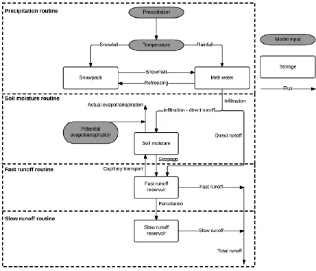
(23) model for assessing climate change impacts as seen from many previous studies (e.g. Tian et al., 2013; Al-Safi & Sarukkalige, 2017; Worqlul, 2018). (Al-Safi & Sarukkalige, 2017) (Worqlul, et al., 2018) (Tian, Xu, & Zhang, Assessment of Climate Change Impacts on River High Flows through Comparative Use of GR4J, HBV and Xinanjiang Models, 2013).. 3.1.2 MODEL DESCRIPTION AND MODEL EQUATIONS In Figure 3-1 the model structure of the HBV-96 model is displayed. The model consists of five storages that are linked together by the fluxes between them. Inputs for the model are the temperature (T) in [oC], potential evapotranspiration (PET) in [mm d-1] and the precipitation (P) in [mm d-1]. The precipitation is also the flux going into the model. Outgoing fluxes are the evapotranspiration (ET) in [mm d-1] and the runoff (Q) in [mm d-1]. The total runoff that is calculated by the model consists of a fast component and a slow component. The fast component is generated from a nonlinear reservoir whereas the slow component is generated from a linear storage box (Bergström, 1992). In the HBV-96 model four routines can be identified: (1) precipitation, (2) soil moisture, (3) fast response and (4) slow response. Each routine is governed by its own model parameters with a total of 14 parameters in the HBV-96 model that can be calibrated.. . FIGURE 3-1: HBV MODEL STRUCTURE, ADOPTED FROM KNOBEN (2013). 18.

(24) Precipitation routine In the precipitation routine the total precipitation is split up into rainfall and snowfall or a combination of the two. At every time step (t) the total precipitation P is divided into rainfall Pr and snowfall Ps based on the air temperature T. Parameters TT in [oC] and TTI [oC] are used to define an interval of size TTI centred around TT along which it is assumed that precipitation will be a mix between rain and snow, linearly decreasing from 100% snow at the lower threshold to 0% snow at the upper threshold. Figure 3-2, adopted from Knoben (2013), gives a visual representation of the TT and TTI parameters and the interval and threshold that they define.. FIGURE 3-2: VISUAL REPRESENTATION OF THE TEMPERATURE INTERVAL AND TEMPERATURE THRESHOLD (KNOBEN, 2013). This distinction between snow and rain allows to direct them to different storage boxes; the snowpack (Ssp) in [mm] and the melt water storage (Smw) in [mm]. The HBV model uses a degree-day approach that, based on air temperature and the water retention capacity of the snow, describes snowmelt (qm) in [mm] (eq. 3.1) and potential refreezing of melt water (qr) in [mm] (eq. 3.2). 𝑞𝑚 (𝑡) = 𝐶𝐹𝑀𝐴𝑋 ∗ (𝑇(𝑡) − 𝑇𝑇) 𝑞𝑟 (𝑡) = 𝐶𝐹𝑅 ∗ 𝐶𝐹𝑀𝐴𝑋 ∗ (𝑇𝑇 − 𝑇(𝑡)). TT CFMAX CFR. (3.1) (3.2). Temperature limit for snow/rain[oC] Degree-day factor of snowmelt [mm OC-1 d-1] Degree-day factor of refreezing [mm OC-1 d-1]. Soil moisture routine The soil moisture routine accounts for the overall wetness of the catchment. Fluxes into the soil moisture routine are capillary transport (qc) in [mm] (eq 3.3) from the fast response routine and infiltration from the precipitation routine. The infiltration is further divided into infiltration (qin) in [mm] (eq 3.4) into the soil moisture storage box (Ssm) and infiltration (qd) in [mm] (eq 3.5) that directly feeds into the fast response storage box (Ssw).. 𝑞𝑐 (𝑡) = 𝐶𝐹𝐿𝑈𝑋 ∗ CFLUX. Maximum rate of capillary flow [mm d-1]. 19. 𝐹𝐶 − 𝑆𝑠𝑚 (𝑡) 𝐹𝐶. (3.3).

(25) 𝑞𝑖𝑛 (𝑡) = 𝑆𝑚𝑤 (𝑡) + 𝑞𝑚 (𝑡) + 𝑃𝑟 (𝑡) − 𝑞𝑟 (𝑡) − 𝑊𝐻𝐶 ∗ 𝑆𝑠𝑝 (𝑡) 𝑞𝑑 (𝑡) = 𝑞𝑖𝑛 (𝑡) + 𝑆𝑠𝑚 (𝑡) − 𝐹𝐶. WHC FC. (3.4) (3.5). Water Holding Capacity of snow [-] Maximum soil moisture content [mm]. Outgoing fluxes from the soil moisture storage are the evapotranspiration (eta) in [mm] (eq 3.6) and seepage (qs) in [mm] (eq 3.7) into the fast response routine storage 𝑒𝑡𝑎 (𝑡) = 𝑒𝑡𝑝 (𝑡) ∗. 𝑆𝑠𝑚 (𝑡) 𝐿𝑃 ∗ 𝐹𝐶. 𝑖𝑓 𝑆𝑠𝑚 (𝑡) < 𝐿𝑃 ∗ 𝐹𝐶 (3.6). 𝑒𝑡𝑎 = 𝑒𝑡𝑝 (𝑡). 𝑖𝑓 𝑆𝑠𝑚 (𝑡) ≥ 𝐿𝑃 ∗ 𝐹𝐶. 𝛽. 𝑆𝑠𝑚 (𝑡) 𝑞𝑠 = ( ) ∗ (𝑞𝑖𝑛 (𝑡) − 𝑞𝑑 (𝑡)) 𝐹𝐶. etp 𝛽 LP. (3.7). Model input, a time series containing the potential evapotranspiration [mm] Soil routine parameter [-] Limit for potential evapotranspiration [-]. Fast runoff response routine The fast runoff response routine has one storage box (Ssw) with five fluxes connected to it. Incoming fluxes are the previously mentioned direct runoff and seepage. Outgoing fluxes are the previously mentioned capillary rise, percolation (qperc) in [mm] to the slow runoff response routine and fast runoff qf in [mm] (eq 3.8) 𝑞𝑓 (𝑡) = 𝐾𝐹 ∗ 𝑆𝑠𝑤 (𝑡)1+𝛼. KF 𝛼. (3.8). Recession coefficient of the fast runoff response reservoir [d-1] Response box parameter [-]. Percolation to the slow runoff response box is not described by an equation but is expressed by parameter PERC describing the amount of water in [mm] that will percolate from the fast runoff response routine storage to the slow runoff response routine storage Sgw. Slow runoff response routine The slow runoff response routine has one reservoir Sgw with one inflow and one outflow. The only inflow into the slow routine is the previously described percolation from the fast runoff response reservoir. The only outflow is the slow runoff qs [mm] (eq 3.9). 𝑞𝑠 (𝑡) = 𝐾𝑆 ∗ 𝑆𝑔𝑤 (𝑡). KS. Recession coefficient of the slow runoff response reservoir [d -1]. 20. (3.9).

(26) 3.2 SENSITIVITY ANALYSIS The HBV model uses 14 parameters in the model routines to translate the model inputs to a runoff value. A risk of a high number of model parameters is that it might result in different parameter sets resulting in a similar model performance, an issue also often referred to as overparameterization (Booij, 2005). To reduce the number of model parameters to be calibrated in the calibration procedure a sensitivity analysis will be applied. The sensitivity analysis will indicate which parameters are most influential for the model performance and should be considered in the model calibration (Song et al., 2015). Measures to assess the performance of a model are found in objective functions. These objective functions give a quantification of how well the model output corresponds to observations. Different objective functions emphasize different parts of the hydrograph. The objective functions that will be used in this research will be described in section 3.2.1. Section 3.2.2 will be used to elaborate on the sensitivity analysis method.. 3.2.1 OBJECTIVE FUNCTIONS Objective functions are used to quantify the quality at which model output resembles the observations. Multiple objective functions are available for this assessment of the goodness of fit. These different objective functions all use different mathematical functions to quantify the quality of the simulations when compared to observations. These differences allow for the different objective functions to focus on different parts of the hydrograph (e.g. peak flows, periods of low flow). Cheng (2014) presents an overview of classical objective functions that are regularly used in hydrological modelling studies. The objective of this research is to find whether there is a trade-off between using different objective functions in model calibration when the aim is to not only simulate the total runoff correctly but also the runoff components. To find this trade-off between objective functions, a weighted combination of two objective functions will be used. From the two objective functions that will be selected, one objective function will put more emphasis on high flow and the other objective function will emphasize low flows. The objective functions that have been selected for this purpose are the Nash-Sutcliffe efficiency criterion (NS) (Nash & Sutcliffe, 1970) and the logarithmically transformed Nash-Sutcliffe efficiency criterion (NSL) (Krause et al., 2005). The NS has been selected because fast runoff has a large contribution to the total runoff during periods of high runoff and runoff peaks, the part of the hydrograph on which the NS puts more emphasis. The NSL on the other hand emphasises periods of low flow more, during these periods baseflow is the dominant runoff component. NS is an objective function that is often used in hydrological modelling studies (e.g. Swamy & Brivio, 1997; Wu & Xu, 2006; Lemonds & McCray, 2007; Benninga et al., 2017; Romanowicz et al., 2016; Osuch et al., 2017). The so-called efficiency that quantifies the quality of the simulation is calculated according to equation 3.10: 2. 𝑁𝑆 = 1 −. ∑𝑖=𝑛 𝑖=1 (𝑄𝑜𝑏𝑠,𝑖 − 𝑄𝑠𝑖𝑚,𝑖 ). 2. ̅̅̅̅̅̅ ∑𝑖=𝑛 𝑖=1 (𝑄𝑜𝑏𝑠,𝑖 − 𝑄𝑜𝑏𝑠 ). (3.10). Where 𝑄𝑜𝑏𝑠,𝑖 denotes the observed discharge at time step 𝑖, 𝑄𝑠𝑖𝑚,𝑖 denotes the simulated discharge at time step 𝑖 and ̅̅̅̅̅̅ 𝑄𝑜𝑏𝑠 is the mean observed discharge. The NS is defined as one minus the sum of the differences between the model output and observations squared and normalized by dividing by the variance of the observations from the considered time period. The value that NS can assume ranges from −∞ to 1 where a NS value of 1 indicates that the simulated discharge exactly agrees with the observed discharge at every time step. Values less than 1 indicate that. 21.

(27) differences between the observed and simulated discharges exist with lower values indicating larger discrepancies between the model output and the observations. Because the NS uses the sum of the differences squared this objective function is more sensitive to high flows. This is a valuable property for assessing the correctness at which peak flows are simulated but can be a limitation when assessing the goodness of the simulation of low flows or baseflow. An objective function that puts more emphasis on low flows is the logarithmically transformed NS (NSL) (Cheng, 2014). Prior to assessing the goodness of the simulation, the observed and modelled hydrographs are logarithmically transformed (eq. 3.11). Following the same methodology as the NS for assessing the correctness of the simulation, this method places more emphasis on low flows compared to the NS (Tesemma et al., 2014). Krause et al. (2015) also presents the NSL as an efficiency criterion that is especially suited for assessing periods of low flow because the influence of high flow values is greatly reduced.. 2. 𝑁𝑆𝐿 = 1 −. ∑𝑖=𝑛 𝑖=1 (log(𝑄𝑜𝑏𝑠,𝑖 ) − log(𝑄𝑠𝑖𝑚,𝑖 )). 2. ̅̅̅̅̅̅ ∑𝑖=𝑛 𝑖=1 (log(𝑄𝑜𝑏𝑠,𝑖 ) − log(𝑄𝑜𝑏𝑠 )). (3.11). 3.2.2 SOBOL’S METHOD A broad palette of methods is available for sensitivity analyses all of different complexities and based on different underlying assumptions on how to correctly assess parameter sensitivity (Song et al., 2005). This can lead to different methods resulting in different results when ranking the parameters based on their relative importance (Frey & Patil, 2002). Sobol’s method for global sensitivity analysis is considered as one of the more robust methods available (Tang et al., 2007). Also, the Sobol method does not rely on model structure or assumptions about the model functioning, e.g. linearity or additivity of the model (Saltelli et al., 2000). The method is classified as a variance decomposition method and results in the overall parameter sensitivity as well as the variance explained by interactions between parameters (Homma & Saltelli, 1996). The goal of this sensitivity analysis is to quantify the contribution of each parameter to the total variance in the model output. This allows the modeler to exclude insensitive parameters from the model calibration by fixing them at a set (default) value (Saltelli et al., 2000). The contribution of variance to the model output by a parameter Xi consists of the main effect, Vi, and the total effect, VTi (Saltelli et al., 2004). These effects are defined by Saltelli et al. (2004) as follows (eq. 3.12 and eq. 3.13): 𝑉𝑖 = 𝑉[𝐸(𝑌|𝑋𝑖 )]. (3.12). 𝑉𝑇𝑖 = 𝑉[𝐸(𝑌|𝑋−𝑖 )]. (3.13). Vi indicates the amount of variance that is contributed to the model result if the true value of only parameter X i was known and the other parameters were allowed to vary. The total effect, V Ti, indicates how much of the variance is left unexplained if the exact values of all the parameters except Xi were known.. 22.

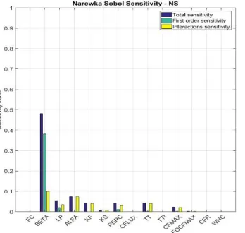
(28) The sensitivity of the parameters can be found by dividing the two variance components by the total output variance V(Y) (eq. 3.14 and eq. 3.15). Where Si is the sensitivity to first order term and STi denotes the total sensitivity index which is a summation of the main effect and interactions with other parameters. The influence of the interactions between parameters on the output sensitivity is determined according to equation 3.16.. 𝑆𝑖 =. 𝑉[𝐸(𝑌|𝑋𝑖 )] 𝑉(𝑌). (3.14). 𝑆𝑇𝑖 =. 𝐸[𝑉(𝑌|𝑋−𝑖 )] 𝑉(𝑌). (3.15). 𝑆𝑖𝑛𝑡𝑒𝑟𝑎𝑐𝑡𝑖𝑜𝑛 = 𝑆 𝑇𝑖 − 𝑆𝑖. (3.16). A sensitivity analysis package was provided by the Polish Academy of Sciences, Institute of Geophysics which, among others, included the Sobol method. The Sobol sensitivity analysis was run for all three catchments for both the NS and the NSL objective functions (section 3.3.2). Every simulation was run using 30 000 samples and used the 30 years of the observational data covering the years 1976 until 2005 that will also be used for model calibration. This resulted in sensitivity indices for all 14 parameters in every catchment for both the objective functions. Determining appropriate thresholds above which parameters are considered for model calibration and below which parameters will be set to a default value is generally an arbitrary decision (e.g. Bastidas et al., 1999; Tang et al., 2007; Knoben, 2013). Here, similarly, the decision on which parameters to include in the model calibration and which ones to fix at a default value will be a subjective one. Using the outcomes of the sensitivity analysis we can classify the model parameters in three main groups based on the amount of variance they explain and therefore also their necessity to be calibrated: -. Parameters that have a high main effect: these parameters influence the overall model performance independently of interaction with other model parameters; Parameters that have a small main effect but a high total effect: these model parameters mainly influence the model performance through interactions with other parameters; Parameters that display a small main effect and a small total effect: these parameters have a negligible effect on the overall model performance and freezing these parameters to their default value is justified (Saltelli et al., 2004).. It is aimed to reduce the number of model parameters that will be calibrated to 8 by taking the parameters that displayed the highest sensitivity from the sensitivity analysis. The choice on which parameters to include will be made based on the total sensitivity index.. 23.

(29) 3.3 MODEL CALIBRATION In this chapter the approach that is taken to calibrate the HBV model is presented. Firstly, the choice on which calibration algorithm will be applied is presented in section 3.1.1. The calibration algorithm that is decided on and will be applied in this research is presented in section 3.3.2 and the periods that will be used for model calibration and validation presented in section 3.3.3.. 3.3.1 CALIBRATION ALGORITHM CHOICE During the calibration procedure the aim is to find the parameter set that allows the model to generate a model output that resembles the observations as closely as possible. To find this parameter set, the Shuffled Complex Evolution Metropolis (SCEM-UA) calibration algorithm will be used (Vrugt et al., 2003a). The SCEM-UA algorithm is a further development of the work of Duan et al. (1992) who presented the SCE-UA algorithm for calibration (of conceptual rainfall-runoff models). The SCE-UA algorithm combines elements from several optimization strategies into one algorithm. Numerous case studies have demonstrated the robustness and efficiency of the SCE-UA algorithm in finding the global optimum. The difficulty for the SCE-UA algorithm is identifying a unique best parameter set that performs significantly better than other feasible parameter sets in its proximity (Vrugt et al., 2003b). Calibration of the HBV model will be done by using the precipitation, the potential evapotranspiration and the temperature observations as model inputs. The model outputs will be evaluated against the discharge observations by using the objective functions described earlier in section 3.2.1. To be able to identify a trade-off between the two objective functions (section 3.2.1), weights will be assigned to both the objective functions during the model calibration. The weights assigned to both objective functions are varied from 0% to 100% with increments of 10% while keeping the sum of the weights equal to 100%. For each of the combination of weights assigned to the objective functions an optimum parameter set will be found resulting in a total of 11 best performing parameter sets per catchment. Before calibration of the HBV model will be done an exploratory Monte Carlo (MC) analysis will be done to determine the appropriate parameter ranges. The parameters that will not be considered in the calibration have been set to their default values according to the HBV manual version 5.10 (SMHI, 2006). For the parameters that will be calibrated preliminary parameter ranges are adopted from Benninga (2017) and Osuch et al. (2016). In the MC analysis the performance of 250 000 parameter sets will be evaluated where each parameter that will be calibrated is individually sampled from a uniform distribution. For each sample the NS and NSL values are then calculated from the output of the HBV model. By evaluating how individual parameter values from the MC samples relate to NS and NSL achieved by the according parameter set, parameter ranges can be adjusted to more appropriate ranges whilst still taking into account their physical meaning and interpretation. 3.3.2 CALIBRATION ALGORITHM The SCEM-UA algorithm applies Markov Chain Monte Carlo (MCMC) sampling following the Metropolis Hastings (Metropolis et al., 1953) strategy instead of the Downhill Simplex procedure, used in the SCE-UA algorithm, for evolution of the population. This change allows the algorithm to find the most likely parameter set as well as its posterior probability distribution. Vrugt et al. (2003a) describe the steps that are involved in the process of finding the ‘best’ parameter set. From the feasible parameter space bounded by the parameter minimum and maximum values, the SCEM-UA algorithm randomly draws the initial population and ranks the sample points in descending posterior density. These initial sample points also serve as the initial points from where the parallel chains will start to evolve. Proposal points for evolving the chain into the next generation are drawn from the proposal distribution that corresponds to the individual chain. The posterior distributions of the new generations are then evaluated and can be either accepted or rejected. If the proposed evolution is accepted the chain then progresses to the new 24.

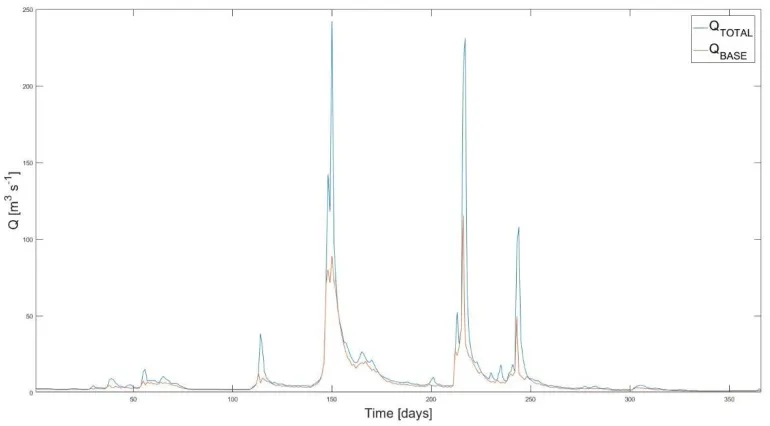
(30) position. If the proposed evolution is not accepted the chain remains at the current position. After every evolution it is checked for convergence according to the Gelman Rubin convergence statistic (Gelman & Rubin, 1992).The calibration process is terminated if either the Gelman Rubin convergence criteria is satisfied or if the predefined maximum number of iterations has been executed. The default settings for the SCEM-UA algorithm are adopted from Vrugt et al. (2003b) and are presented in Table 3-1. TABLE 3-1: SCEM-UA ALGORITHM PARAMETERS (VRUGT ET AL., 2003B). Setting Description nSamples Population size nCompl The number of complexes nModelEvalsMax The maximum number of model iterations drawInterval Shuffling rate of complexes 3.3.3 CALIBRATION AND VALIDATION PERIOD. Value 200 5 10 000 5. The provided datasets by the IGF PAN consist of 40 years of continuous observations spanning from 1 January 1971 until 31 October 2010. The dataset is used for two purposes, namely: (1) calibration of the HBV model and (2) validation of the HBV model. To prevent biased results periods have been defined that do not overlap. Model calibration using the SCEM-UA algorithm will be done using the observations between 1 November 1976 and 31 October 2005. The validation of the model calibration will be done by applying a split-sample test (Klemeš, 1986). The split-sample test will be done using the observational data from 1 November 2005 until 31 October 2010.. 3.4 SIMULATION OF RUNOFF COMPONENTS There is widespread agreement that for assessing model performance the correspondence between the total measured and modelled stream flow is not a sufficient indicator. Additional insights in the processes that take place within the catchment would be a step towards improvement of runoff modelling (Beven, 1989). Yet, in most cases the assessment of model performance is still done based on the total runoff because individual components that contribute to the total runoff usually go unobserved. The information that observed hydrographs provide however, is not limited to the absolute values of the measured runoff. Eckhardt et al. (2002) presents an example of what the potential benefits of having insight in the runoff components can provide for model performance.. 3.4.1 HYDROGRAPH SEPARATION Over the years, many methods have been developed that allow for the identification of the baseflow component from the total runoff e.g. low-pass filtering, recursive filtering and unit hydrograph methods. Often linear reservoirs have been used for modelling the groundwater contribution, i.e. baseflow, to the total flow (e.g. Chapman. 1999; Fenicia et al., 2006; Eckhardt, 2005). More recent studies however by Wittenberg (1994, 1999, 2003), Gan & Luo (2013) and Aksoy et al., (2008) have used nonlinear reservoirs for the analysis of groundwater recession and baseflow contribution as these methods appeared to give a more realistic representation of catchment processes. Baseflow separation in this research is done according to the non-linear reservoir approach from Wittenberg (1999). Wittenberg’s baseflow separation method assumes a power-law relationship between the baseflow and the groundwater storage of the catchment (eq. 3.17). With S denoting the groundwater storage and Q representing the recession of the baseflow and 𝑎 and 𝑏 are model parameters. Parameters 𝑎 and 𝑏 for flow recessions are found by an iterative process by calibrating them against flow recession data by utilizing a least-squares method (Wittenberg, 1999). 𝑆 = 𝑎 ∗ 𝑄𝑏 25. (3.17).

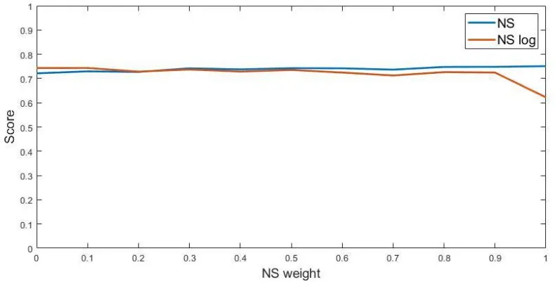
(31) The analytical solution for the baseflow is presented by Wittenberg (1999) and is given in equation 3.18. Here QB indicates the baseflow resulting from the nonlinear reservoir at time step t starting from initial discharge Q0. 1. 𝑏−1 (1 − 𝑏) ∗ 𝑄01−𝑏 𝑄𝐵 = 𝑄0 [1 + ∗ 𝑡] 𝑎𝑏. (3.18). With the contribution of the baseflow to the total flow determined by applying Wittenberg’s baseflow separation method the fast runoff (QF) component can easily be found by subtracting the baseflow component from the total flow (QT) (eq. 3.19). (3.19) 𝑄𝐹 = 𝑄𝑇 − 𝑄𝐵 To illustrate the results of the hydrograph separation the hydrograph separation done for the Biała Tarnowska catchment for the year 1976 is graphed and presented in Figure 3-3. It shows that during periods of low flow the runoff almost entirely consists of baseflow and that fast runoff barely contributes to the total runoff. During high runoff events it is observed that the baseflow also increases but the main contribution to the total flow becomes the fast runoff component.. FIGURE 3-3: WITTENBERG'S BASEFLOW SEPARATION APPLIED TO THE BIALA TARNOWSKA CATCHMENT FOR THE YEAR 1976. 3.4.2 SIMULATION OF RUNOFF COMPONENTS Determining model performance in simulating the runoff components will be done by comparing the runoff components derived from the observed runoff for the calibration period with the runoff components derived from the simulated runoff for the calibration period. This is done for each simulation using the different parameter sets that resulted from model calibration (section 3.3). Assessing the correctness of the simulated runoff components for the previously determined parameter sets will be done by using the previously described NS objective function (section 3.2.1). Identifying a trade-off between using different objective functions and the model its ability to correctly simulate the runoff components will be done by checking if there is a correlation between the weights assigned to the objective 26.

No results found