A Bootstrapping Approach for Software Reliability Measurement Based on a Discretized NHPP Model

A Bootstrapping Approach for Software Reliability

Measurement Based on a Discretized NHPP Model

Shinji Inoue, Shigeru Yamada

Department of Social Management Engineering, Graduate School of Engineering, Tottori University, Tottori, Japan. Email: [email protected], [email protected]

Received December 14th_{,2012; revised January 17}th_{, 2013; accepted January 26}th_{, 2013}

Copyright © 2013 Shinji Inoue, Shigeru Yamada. This is an open access article distributed under the Creative Commons Attribution License, which permits unrestricted use, distribution, and reproduction in any medium, provided the original work is properly cited.

ABSTRACT

Discrete software reliability measurement has a proper characteristic for describing a software reliability growth process which depends on a unit of the software fault-detection period, such as the number of test runs, the number of executed test cases. This paper discusses discrete software reliability measurement based on a discretized nonhomogeneous Poisson process (NHPP) model. Especially, we use a bootstrapping method in our discrete software reliability meas-urement for discussing the statistical inference on parameters and software reliability assessment measures of our model. Finally we show numerical examples of interval estimations based on our bootstrapping method for the several software reliability assessment measures by using actual data.

Keywords: Software Reliability Measurement; Discretized NHPP Model; Nonparametric Bootstrapping Method;

Regression Analysis; Bootstrap Confidence Intervals

1. Introduction

It is very important to measure reliability of a software product with accuracy in the final stage of software de- velopment process for shipping a highly reliable software product. A software reliability growth model [1-4] is known as one of the useful mathematical tools for quan- titative measurement or assessment of software reliability. Generally in an actual testing-phase, we observe a soft- ware reliability growth process, in which software faults are detected and removed and the number of faults re- maining in the software system is decreasing along with the test-execution time. The software reliability growth model describes the software reliability growth process, and measures the software reliability quantitatively by using software reliability assessment measures, which are derived by the software reliability growth model. A huge number of software reliability growth models were pro- posed so far for accurate software reliability assessment. Especially, there are discretized nonhomogeneous Pois- son process (discretized NHPP) models, which have good fitting and prediction performance in software reli- ability assessment [5,6] because the discretized NHPP models have consistency with fault counting data, which are obtained by collecting information on the frequency of the software failure-occurrence or the number of detected

faults during each constant testing-period. Estimating parameters in the discretized NHPP model from actual data is conducted by using the regression analysis based on a regression equation derived from a difference equa- tion of the discretized NHPP model. After the parameter estimation, software reliability assessment is performed based on the software reliability assessment measures derived from the discretized NHPP model. This approach is based on the point estimation, which is better to use when we have enough number of data.

the bootstrapping method is applied not only to software reliability analysis [9-11] but also optimal checkpoint replacement for hardware system [12].

In this paper, we discuss an interval estimation method for parameters and software reliability assessment meas- ures of a discretized exponential software reliability growth model, which is one of the discretized NHPP mo- dels and has the simplest model-structure, by the boot- strapping method. And, we discuss several kinds of boot- strap confidence intervals for the interval estimations. Finally, we show numerical examples for our bootstrap- ping method for software reliability assessment based on the discretized exponential software reliability model and the bootstrap confidence intervals by using actual data.

2. Discretized Exponential NHPP Model

2.1. The Model

We briefly discuss the aspect of the discretized NHPP model by showing a discretized exponential software reliability growth model [5,6], which has the simplest mathematical structure. Now we define a discrete

count-ing process representing the

cumula-tive number of faults detected up to n-th testing-period.

And we can say that the discrete counting process

n follows a discrete-time NHPP [13] if

the process has the following property:



Nn,n0,1, 2,



,1, 2,





N ,n0





 

_

_

_

0

Pr | 0

exp , 0,1, 2, ,

!

n x n

n

N x N

n x



x

 



    (1)

which is derived based on a continuous-time NHPP. In

Equation (1), Pr

 

A means the proba of event A. _n

is a mean value function of the discrete-time NHPP. The

mean value function, n, represents the expected

cu-mulative number of faults detected up to nth

test-ing-period.



The discretized exponential software reliability growth model is a discrete analog of the original (continu-ous-time) exponential software reliability growth model.

Let Hn denote the mean value function following the

discretized exponential software reliability growth model. The discretized exponential software reliability growth model is given as





1 ,

n n n

H _ H  H (2)

from the basic assumptions of the original exponential

software reliability growth model. In Equation (2), 

represents the constant time-interval,  the expected

total number of potential faults to be detected in an infi-nitely long duration or the expected initial fault content,

and  the fault detection rate per fault. Regarding the

discretization method, we use the Hirota’s bilinearization

methods [14] for conserving the property of the continu-ous-time NHPP model. Solving the integrable difference equation in Equation (2), we can obtain an exact solution

n

H as







1 1 n 0, 0 .

n

H _   _   

0



(3)

As   , Equation (3) converges to an exact

solu-tion of the original continuous-time exponential software reliability growth model, which is derived by the differ-ential equation.

The discretized exponential software reliability growth

model in Equation (3) has two parameters,  and ,

which have to be estimated by using actual data. The

parameter estimations of  and  , ˆ and ˆ, can

be obtained by the following procedure using the method of least-squares. First of all, if we observed fault count-ing data



n y, n





n1, 2,,N



, where n represents

the cumulative number of faults detected up to nth

test-ing-period, we derive the following regression equation from Equation (2):

y

0 1 ,

n

C   D_n (4)

where

1 1

0

1 .

n n n n

n n n

C H H y y D H y

 

 

  n

   



 _{ }



 _

    

(5)

Based on the regression analysis, we can estimate ˆ0

and ˆ1, which are the estimations of 0 and 1 in

Equation (4). Then, the parameter estimations, ˆ and

ˆ

, can be obtained as

0 1

1

ˆ ˆ ˆ

ˆ _{ˆ .}

  

  

   

 

 (6)

n in Equation (4) is independent of

C  because 

is not used in calculating n as showing Equation (5).

Hence, we can obtain the same parameter estimates

C

ˆ



and ˆ, respectively, when we choose any value of 

[5,6,15,16].

2.2. Software Reliability Assessment Measures

Software reliability assessment measures are useful in quantitative software reliability assessment. This paper discusses the expected number of remaining faults and the software reliability function, which are well-known software reliability assessment measures. The expected

number of remaining faults, Mn, represents the ex-

pected number of undetected faults in the software system at arbitrary testing-period. Then, we have







1



n

n n n

M   NN       , (7)

with mean in Equation (3). The software reliability

function, , is defined as the probability that a

software failure does not occur in the time-interval n





,

R n h





n n, h





h1,

R n



2,

 

h



, P

given that the testing has been

going Up to the nth testing-priod. Then, we have













r 0 |

exp

exp 1 .

n h n n

n h n

n h

N N N x

H 





   

 

 _    _

 

 _  _

(8)

3. Software Reliability Assessment Based on

Bootstrapping Method

Ordinarily, the parameters of the discretized NHPP mo- dels are estimated by using the regression analysis based on the regression equation derived from the difference equation of the discretized NHPP models. However, it is difficult to discuss the statistical inference on software reliability assessment in the existing estimation approach because it is very difficult or complex to identify the probability distribution function for the estimators of pa- rameter analytically. For overcoming a problems above, Kimura and Fujiwara [9,10] applied non-parametric boot- strap software reliability assessment methods for an in- complete gamma function-based software reliability growth model. Kaneishi and Dohi [11] discussed a parametric bootstrap method for software reliability assessment based on continuous-time NHPP models. In this paper, we ap- ply a non-parametric bootstrap method to the discretized NHPP model for estimating model parameters and for obtaining information for the statistical inference on the parameters and software reliability assessment measures. Especially in this paper, we discuss five types of boot- strap confidence intervals for interval estimation of the model parameters and software reliability assessment measures.

3.1. Our Bootstrapping Method

As an example for discussing our bootstrapping method based on the discretized NHPP model, we apply the dis- cretized exponential software reliability growth model. Our bootstrap method for software reliability assessment follows the following procedure:

Step 1: Estimate 0 and 1 in Equation (4) based

on the linear regression scheme by using fault counting data. We indicate ˆ0 and ˆ1 as ˆ0 0  and ˆ1 0 , res- pectively.

Step 2: Calculate the residual errors, at each

observation point by

ˆ

i

d

  0 0  



ˆ ˆ1 0Di





i1, 2, , N1 .



ˆ

ˆ

i i

d C 

Step 3: Construct an empirical distribution function

F by assuming the residual errors follows the

independent and identically probability distribution and putting mass

ˆ

i

d





1 N1 at each ordered point

     



dˆ1,dˆ2, , dˆN1



.

Step 4: Set the total number of iteration B and let

b



b1, 2, , B



be the iteration count.

Step 5: Generate a bootstrap sample for the residual errors,

 



,1 ,2 , 1



ˆ ˆ _,ˆ _{, ,}ˆ

b b b N

b

d  d d  d _

by sampling with replacement from Fˆ .

Step 6: Generate a bootstrap sample for

 b





1, b,1

 

, 2, b,2

 

, , N 1, b N, 1





z  y C y C  y _ C _

by

   

, ˆ0 0 ˆ1 0 ˆ,.

b i i b i

C   D d

Step 7: Estimate ₀_{ b and}

 

1b

 _{from the bootstrap}

sample z_{ }_b .

Step 8: Calculate parameters of the discretized expo- nential software reliability growth model by the fol- lowing equation:

   

 

   

0

1

1 ˆ ˆ ˆ

. b b

b

b b

 

  



 



 

 

 

Step 9: Calculate software reliability assessment measures.

Step 10: Let b b 1 and go back to Step 5 if. b < B

Step 11: We have B samples for ˆ , ˆ and a

software reliability assessment measures.

We can calculate the mean and the standard deviation for the model parameters and software reliability assess- ment measures by the Monte Carlo approximation, re- spectively.

3.2. Bootstrap Confidence Intervals

We discuss the following three typical bootstrap confi- dence intervals [17]: basic, standard normal, and per- centile bootstrap confidence intervals. Further we discuss

bootstrap-t and BCa methods [17,18] for deriving boot-

strap confidence intervals considering with the asym- metric property and the bias and the skewness of the esti-

mator of the parameter. Let  be parameter of interest.

The basic bootstrap confidence interval is derived by using the quantile of the distribution of ˆ_ˆ_{, where}

ˆ

 _{is the bootstrap statistic. We can approximate the }

and



1



quantile denoting va and va-1, respec- tively,

of the distribution of ˆ  by ˆ_{ }_{B }ˆ _and

1 

ˆ ˆ

B 

 



 









   



1 1 1 ˆ

1 2 Pr

ˆ ˆ

Pr

ˆ ˆ ˆ

Pr 2 _B 2 _B .

v v v v                                   

     ˆ



.





Thus, the basic bootstrap confidence

interval is given by





100 1 2  %

1   

ˆ ˆ ˆ ˆ

2  B  , 2 B

 

 

 

 _{ } 

 (9)

The standard normal bootstrap confidence interval is

derived by assuming that the distribution of ˆ  can

be approximated by the distribution of ˆ_ˆ _and



2



ˆ _{ˆ ~N 0,SD}

_ _{ }

 ˆ . That is,

1

ˆ ˆ

1 2 Pr

ˆ w w SD          _      _   _    _{ }    .

Thus, we have the standard normal

bootstrap confidence interval as





100 1 2  % 1

ˆ _{w SD} ˆ _, ˆ _{w SD}

 

 _  

   _{ }   _{ }

 ˆ , (10)

where w_ is 1

 

 , which is the  quantile of the

standard normal distribution. For example,

1 0.025 0.025 1.96

w_  w  .

The percentile bootstrap confidence interval is calculated from the empirical cumulative probability dis- tribution function, which consists of the bootstrap itera- tion values:  ˆ_{   }₁,ˆ₂ , ,ˆ_{ }_B . Then, the

percentile bootstrap confidence interval is calculated by





100 1 2  %

  1 

ˆ _, ˆ

B B 

 



 

 



 , (11)

where ˆ_{ }_B represents the  quantile of the empirical cumulative probability distribution function.

Further, we discuss a bootstrap-t method, which

enables us to take into consideration the variance of ˆ

by deriving T

 

  ˆ ˆ, where ˆ2 is the variance of ˆ. Letting u_ and u_{1} are the  and



1



quantile of T, we have



1

1 ˆ

1 2 Pr

ˆ

ˆ _ˆ ˆ _ˆ

Pr . u u u u                       _   _         



In above equation, we substitute u and u1, which are  and



1



quantile of T , into T_{ B}_ and

1  B T_ _

 , which are the  and



1



quantile of



ˆ ˆ



_ˆ

T    

.



  _{. Then, the}

bootstrap-t

confidence interval is derived as





100 1 2  %

1   

ˆ _{ˆ ,} ˆ _ˆ

B B

T _ T _

    



 

 

 _{ } 

  (12)

In Equation (12), ˆ is the standard deviation of ˆ_{ }_b

and ˆ is estimated by the bootstrap-t statistics T.

And we also discuss a BCa method for getting better

bootstrap confidence interval with the asymmetric property, the bias, and the skewness of the probability

distribution of the estimator. The BCa confidence

interval can be given as

 





















1 1

ˆ _, ˆ ₁

G z  G z  ,

 _{  } 

  (13)

where

 

0

_

_

0

0 1

z z

z z

a z z





   

  .

In above equation, 1



 

0 ˆ ˆ

z   G 



, in which Gˆ

 

 is

the bootstrap distribution for the estimator. And is the acceleration constant derived as

a    





   





3 1 3 2 2 1 ˆ ˆ 1

6 _{ˆ ˆ}

n i i n i i a            _     





,

where ˆ_{ i} is a jackknife iteration value, which is

estimated by using the data, removed ith data and

  1ˆ

n i

ˆ _

i n

 



.

4. Numerial Examples

We show numerical examples for our bootstrap software reliability assessment method based on the discretized exponential software reliability growth model.

We apply fault counting data:



n y, n





n1, 2, , 25; y25 136



2000

B

 [1] and we set the total

num-ber of iteration  .

We first obtain   0 0

ˆ 139.9564

  and ˆ_{1 0 }0.1133109 by the linear regression scheme from the actual data. Following to our bootstrapping method, we have 2000 bootstrap samples



z_{   }₁,z₂, , z__2000



. Then, we obtain

bootstrap samples for  and  . Figures 1 and 2 show

histograms for the bootstrap samples ˆ_{ }_{b and}

 

ˆ

b

 _to

see bootstrap distributions of ˆ and ˆ, respectively.

And we have bootstrap samples for the software reliabil-ity assessment measures, such as the expected number of remaining fault at the termination time of the testing,

25

ˆ

M , and the software reliability, Rˆ 25



,1



, respectively.

These bootstrap samples of Mˆ25_{ }b and



 b



25,1





ˆ

R are

calculated by      



  25 0 * 25 1 1 ˆ

ˆ _{1 ˆ}

ˆ

b b

b

M   _b



  



  , (14)

 





   





 







 



1 0 1 1 1 ˆ

ˆ _{25,1 exp 1 1 ˆ 1 ˆ ,}

ˆ

n b

b b

b

R   

     b           

[image:5.595.57.288.77.541.2] [image:5.595.309.537.84.290.2]

Figure 1. Bootstrap distribution of ˆ.

Figure 2. Bootstrap distribution of ˆ.

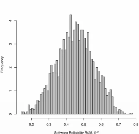
From Equations (7) and (8), respectively. Figures 3

and 4 show histograms of the bootstrap samples for

 

25 and   , respectively. Further, Table 1

indicates the mean and the standard deviations of the

estimators of 0

ˆ

b

M Rˆ_b



25,1

ˆ



 , ˆ1, ˆ, ˆ , Mˆ25, and Rˆ 25,1





ˆ

n

,

respectively. And, Figure 5 shows the estimated

discre-tized exponential software reliability growth model, H ,

in which we use the means of the bootstrap samples of  

ˆ_b

 _and

  ˆ

b



ˆ_b

as the point estimations, respectively.

The means of _{ } _and

 ˆ

b

 _{, which are denoted by }

and  , are calculated by

 

1

1 B _{ˆ ,}

b b

B

 







(16)

[image:5.595.59.285.86.309.2]

Figure 3. Bootstrap distribution of the expected number of remaining faults at n = 25,Mˆ25.

Figure 4. Bootstrap distribution of software reliability, .

ˆ_(25,1)

R

 

1

1 B _{ˆ ,}

b b

B

 







(17)

respectively.

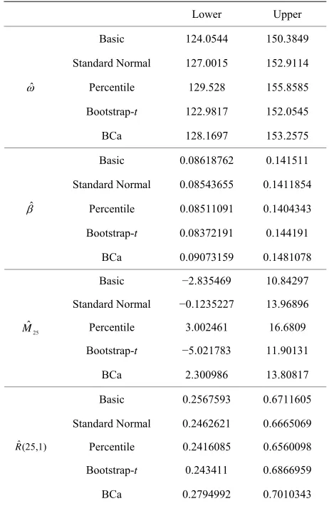
Further, Table 2 shows the results of interval estima-

tions based on the basic, standard normal, percentile,

bootstrap-t, and BCa methods, respectively, with the 5%

significance level



0.025



. From Table 2, we can

see that the inappropriate confidence intervals for Mˆ25

are estimated in the basic, standard normal, and boot-

[image:5.595.310.538.336.556.2]

[image:6.595.57.290.69.291.2] [image:6.595.307.538.111.466.2]

Figure 5. Estimated discretized exponential software re- liability growth model,Hˆn.

Table 1. Quantities of the bootstrap distribution.

Mean Standard Deviation

0

ˆ

 15.79443 1.500837

1

ˆ

 −0.1127263 0.01422163

ˆ

 140.7685 6.609685

ˆ

 0.1127263 0.01422163

25

ˆ

M 7.761994 3.59502

ˆ (25,1)

R 0.4514124 0.1072053

maining faults does not never take a negative value. And depending on the type of the bootstrap confidence inter- val, the results of interval estimations on Mˆ25 are nota-

bly different each other. These results are caused by as- suming the symmetric distributions to derive these boot- strap confidence intervals. However, the probability dis- tribution of an estimator follows an asymmetric distribu- tion and the approximate accuracy is influenced by the bias and the skewness of the probability distribution for

the estimator generally. As we show in Figure 3, we can

say the bootstrap distribution for Mˆ25 follows an asym-

metric distribution. On the other hand, the percentile bootstrap confidence interval give us an appropriate in-

terval estimations on Mˆ25 because the interval estima-

tion based on the percentile method is estimated based on only the bootstrap distribution, not assumed a symmetric distribution. Of course, the interval estimations based on

the BCa method can be thought that we have more ap-

propriate interval estimation on Mˆ25 because the BCa

method is the improved estimation method for the per- centile bootstrap confidence interval.

Table 2. Results of interval estimations based on bootstrap confidence intervals.

Lower Upper

Basic 124.0544 150.3849

Standard Normal 127.0015 152.9114

Percentile 129.528 155.8585

Bootstrap-t 122.9817 152.0545

ˆ



BCa 128.1697 153.2575

Basic 0.08618762 0.141511

Standard Normal 0.08543655 0.1411854

Percentile 0.08511091 0.1404343

Bootstrap-t 0.08372191 0.144191

ˆ



BCa 0.09073159 0.1481078

Basic −2.835469 10.84297

Standard Normal −0.1235227 13.96896

Percentile 3.002461 16.6809

Bootstrap-t −5.021783 11.90131

25

ˆ

M

BCa 2.300986 13.80817

Basic 0.2567593 0.6711605

Standard Normal 0.2462621 0.6665069

Percentile 0.2416085 0.6560098

Bootstrap-t 0.243411 0.6866959

ˆ (25,1)

R

BCa 0.2794992 0.7010343

5. Conclusions

This paper discussed a bootstrap software reliability as- sessment method based on a discretized exponential soft- ware reliability growth model. And we discussed five types of bootstrapping confidence intervals for interval estimations of model parameters and several software reliability assessment measures.

In our numerical examples, we confirmed that our bootstrap approach gives probability distributions of each parameters and software reliability assessment measures numerically even if we do not derive these probability distributions analytically, and that we can obtain useful information in software reliability assessment, such as results of interval estimations on the model parameters, the number of remaining faults, and software reliability. This approach is very useful for the case that we cannot collect enough number of data and we have to conduct interval estimation for complex estimators. However, regarding bootstrap confidence intervals, we encountered a problem that we could not get appropriate interval

[image:6.595.58.285.349.470.2]

confidence intervals for the number of remaining faults at the termination time of the testing. This problem was solved by using other bootstrap confidence intervals,

such as the percentile and the BCa confidence intervals.

In the future studies, we are going to apply our bootstrap approach for estimating optimal software release time and other practical software project management issues.

6. Acknowledgements

The second author is supported in part by the Grant-in- Aid for Scientific Research (C), Grant No. 22510150, from the Ministry of Education, Culture.

REFERENCES

[1] J. D. Musa, “A Theory of Software Reliability and Its Application,” IEEE Transactions on Software Engineer- ing, Vol. SE-1, No. 3, 1975, pp. 312-327.

doi:10.1109/TSE.1975.6312856

[2] A. L. Goel, “Software Reliability Models: Assumptions, Limitations, and Applicability,” IEEE Transactions on Software Engineering, Vol. SE-11, No. 12, 1985, pp. 1411-

1423. doi:10.1109/TSE.1985.232177

[3] J. D. Musa, D. Iannio and K. Okumoto, “Software Reli- ability: Measurement, Prediction, Application,”McGraw- Hill, New York, 1987.

[4] H. Pham, “Software Reliability,” Springer-Verlag, Sin- gapore, 2000.

[5] S. Inoue and S. Yamada, “Discrete Software Reliability Assessment with Discretized NHPP Models,” Computers & Mathematics with Applications: An International Jour- nal, Vol. 51, No. 2, 2006, pp. 161-170.

doi:10.1016/j.camwa.2005.11.022

[6] S. Inoue and S. Yamada, “Integrable Difference Equa- tions for Software Reliability Assessment and Their Ap- plications,” International Journal of Systems Assurance Engineering and Management, Vol. 1, No. 1, 2010, pp.

2-7. doi:10.1007/s13198-010-0005-x

[7] S. Yamada and S. Osaki, “Software Reliability Growth Modeling: Models and Applications,” IEEE Transactions on Software Engineering, Vol. SE-11, No. 12, 1985, pp. 1431-1437. doi:10.1109/TSE.1985.232179

[8] B. Efron, “Bootstrap Methods: Another Look at the Jackknife,” The Annals of Statistics, Vol. 7, No. 1, 1979, pp. 1-26. doi:10.1214/aos/1176344552

[9] M. Kimura, “A study on Bootstrap Confidence Intervals of Software Reliability Measures Based on an Incomplete Gamma Function Model,” In: T. Dohi and W. Y. Yun, Eds., Advanced Reliability Modeling II, World Scientific,

Singapore City, 2006, pp. 419-426.

[10] M. Kimura and T. Fujiwara, “A Bootstrap Software Re- liability Assessment Method to Squeeze out Remaining Faults,” In: T. H. Kim and H. Adeli, Eds., Advances in Computer Science and Information Technology, Springer- Verlag, Berlin-Heidelberg, 2010, pp. 435-446.

doi:10.1007/978-3-642-13577-4_39

[11] T. Kaneishi and T. Dohi, “Parametric Bootstrapping for Assessing Software Reliability Measures,” Proceedings of the 17th IEEE Pacific Rim International Symposium on Dependable Computing, 12-14 December 2010, pp. 1-9.

[12] S. Tokumoto, T. Dohi and W. Y. Yun, “Toward Develop- ment of Risk-Based Checkpointing Scheme via Paramet- ric Bootstrapping,” Proceedings of the 2012 Workshop on Recent Advances in Software Dependability, 19 Novem-

ber 2012, pp. 50-55.

[13] S. Yamada and S. Osaki, “Discrete Software Reliability Growth Models,” Journal of Applied Stochastic Models and Data Analysis, Vol. 1, No. 1, 1985, pp. 65-77. doi:10.1002/asm.3150010108

[14] R. Hirota, “Nonlinear Partial Difference Equations. V. Nonlinear Equations Reducible to Linear Equations,”

Journal of the Physical Society of Japan, Vol. 46, No. 1, 1979, pp. 312-319. doi:10.1143/JPSJ.46.312

[15] D. Satoh, “A Discrete Gompertz Equation and a software Reliability Growth Model,” IEICE Transactions on In- formation and Systems, Vol. E83-D, No. 7, 2000, pp.

1508-1513.

[16] D. Satoh, “A Discrete Bass Model and Its Parameter Es- timation,” Journal of the Operations Research Society of Japan, Vol. 44, No. 1, 2001, pp. 1-18.

[17] M. L. Rizzo, “Statistical Computing with R,” Chapman and Hall/CRC, Boca Raton, 2008.

[18] B. Efron, “Better Bootstrap Confidence Intervals,” Jour- nal of the American Statistical Association, Vol. 82, No. 397, 1987, pp. 171-185.