4059
TEXTURE PATTERN IN ABNORMAL MAMMOGRAMS
CLASSIFICATION USING SUPERVISED MACHINE
LEARNING TECHNIQUES
1YOUSSEF BEN YOUSSEF, 1ELHASSANE ABDELMOUNIM, 2ABDELAZIZ BELAGUID,
3MOHAMMED NAJIB BOUJIDA
1Department of Applied Physics, Faculty of, Sciences and Techniques Settat, Morocco
2Laboratory of physiology, Faculty of medicine and Pharmacy Rabat, Morocco
3Professor in Faculty of medicine and Pharmacy, head of department of Radiology in Institute of Oncology
Moulay Abdellah, CHU Ibnou Sina,Rabat, Morocco.
E-mail: 1[email protected], 1[email protected] ABSTRACT
The purpose of the present study is to extract pattern texture from regions of interest (ROI) on mammograms and to use texture descriptors to classify the ROI into benign or malignant mammograms. Supervised Machine Learning (SML) algorithms like Support Vector Machine (SVM) and Multi-Layer Perceptron (MLP) are used to classify the ROI. Two types of texture descriptors (GLCM and GRLM) are extracted after cropping and resizing the ROI. The goal is to find the best texture descriptors which give best accuracy in the classification of mammogrames.
Our proposed method is proved to be a highly efficient method for the diagnostic of breast cancer with high accuracy using SVM. This study proves that SVM is a consistent classifier for two mammogram databases use.
Keywords: Breast cancer, Computer Aide Diagnosis (CAD), Classification, Supervised Machine Learning(SML), Texture Pattern
1. INTRODUCTION
One of the leading causes of cancer related death in women is breast cancer in all countries. But Breast cancer early detected is easier to treat successfully. Clinical breast examination associated with mammography is the most efficient method for early detection of breast cancer and for decreasing breast related mortality [1].
In their daily routine, radiologists perform a classification task by labelling the abnormal mammogram as benign or malignant after detecting a lesion. However, a considerable number of biopsy examinations give negative results.
In screening mammography, a huge number of images is generated. The perception of small details of breast and the recognition of meaning of these details are the weakest links in mammographic image interpretation. In this context, reading or interpreting is a difficult task for radiologists. Their judgments depend on training, experience, and subjective criteria. Even well-trained experts may have an inter-interpretation variation rate of 65%-75%[2]. According to [3], 10%–25% of abnormal cases shown in mammography have been ignored by radiologists.
These problems yield a lower quality of result diagnosis provided by human expert. SML techniques are used to support decision-making and problem-solving applications. Their benefits include, enhanced problem-solving, improved decision quality, ability to solve complex problems and consistent decisions.
In order to increase efficiency and more accurate diagnosis, the use of computer vision systems become paramount. The aim of embedding computers in mammography is to build a Computer Aided Diagnosis (CAD) system in mammography. The CAD is objective, faster, tireless, and does not have the limitations of the human visual system.
Computer Aided Diagnosis(CAD) system developed within computer image analysis and SML techniques is a promising way.
4060 design systems that perform automatic classification. The ability of SML to learn from descriptors of given class patterns and to classify the unknown patterns of such classes into appropriate classes using the acquired knowledge shown its potential in the field of pattern recognition.
Among descriptors used in image analysis and understanding, texture information plays an important role with potential applications as in remote sensing, medical diagnosis and many other application areas [6]-[7]. Moreover it is believed that human visual systems unconsciously use texture for recognition and interpretation [8]. The rest of this paper is organized as; Section 2 presents research objectives; Section 3 discusses the related work, Section 4 reveals the basic theory and some useful properties of pattern texture and some measure of descriptors extracted. In Section 5, we describe supervised machine learning algorithms used in this work like SVM and MLP for classification, while Section 6 describes methodology and the proposed method. The experimental results obtained by the proposed method and discussion are presented in section 7. In the last section, a conclusion is made and highlights both limitations and future directions.
.
2. REESERCH OBJECTIVES
The aim of this paper is to extract pattern texture from regions of interest (ROI) i.e. masses on mammograms and to use texture descriptors to classify the masses (ROI) into benign or malignant. Supervised Machine Learning (SML) algorithms like Support Vector Machine (SVM) and Multi-Layer Perceptron (MLP) are used to perform the classification and compare their results in terms of accuracy.
The performance of this method is measured by the accuracy which can be viewed as the ratio of the number of mammograms correctly classified over the total number of test mammograms using texture descriptors as input to machine learning techniques.
The mammogram database used is a set of 40 mammograms: 20 mammograms are selected from the Mini Mammographic Image Analysis Society (MIAS) database which is the most commonly used as a standard test database for researchers to be able to directly compare their results. Most of the mammographic databases are not publicly available; and 20 mammograms are produced by the National Institute of Oncology (NIO) Moulay Abdellah, of Mohammed V University in Rabat Morocco [9] as a first step to develop a new project of Moroccan mammographic image database. 22
test mammographic images are benign and 18 mammographic images are malignant. Finally, our study deals with mammograms classification using SVM and MLP and comparing their performance.
3. RELATED WORK
Many researchers have contributed significantly towards the classification of mammogrames in order to improve the diagnosis classification rate and to reduce the load of radiologists and facilitating them with computer aided diagnosis system.
Yuvaraj and Ragupathy proposed a method for segmentation and classification of mammographic masses. They collected mammogram images from Imaging Centre, Coimbatore and from MIAS database. Histogram equalization method was used for enhancement of regions of suspicion of size 256×256, and segmentation was done with iterative active contour method. They used GLCM based statistical method for feature extraction, which were input to Adaptive Neuro Fuzzy Interface System (ANFIS) and achieved an accuracy of 91.3%.[10].
Recently Several system based on Computer Aided Detection and Diagnosis (CAD) for breast cancer are proposed by researchers and more techniques for classification are used to evaluate
their performances as support vector
machines(SVM), and neural networks and others[11].
Mavroforakis et al. proposed a quantitative approach for mass classification based on advanced classification architecture and supported by fractal analysis dataset of extracted texture descriptors. Fractal analysis was employed to compare information content and dimension ability of texture feature datasets with quantitative information provided though medical diagnosis. The best mass classification of mammogram based only texture features achieved an optimal score of 83.9% by using SVM classifier [12].
Liu and Tang extracted geometrical and texture features. They used features extracted from band around the closed contour of the mass and integrated a support vector machine (SVM) based recursive feature elimination procedure with normalized mutual information; the proposed method achieved 94% of accuracy [13].
4. PATTERN TEXTURE DESCRIPTORS
EXTRACTION
4061 placement rules. In this approach, it is suitable for deterministic textures [14]; (ii) stochastic approach considers textures as realisations of a random process describable by its statistical parameters [15]; (iii) statistical approach where sets of statistics can be obtained to characterize these patterns. Spatial grey-level matrix based on studies of the arrangement of pixel and relationship between a pixel and its neighbours is taken into consideration [16]-[17].
Pattern texture descriptors can be broadly classified into spatial texture descriptor extraction methods and spectral texture descriptor extraction methods. Spatial texture descriptors are extracted by calculating the pixel statistics or finding the local pixel structures in original image domain while spectral texture descriptors are calculated after transforming image in frequency domain. Spectral texture descriptors need square image regions with sufficient size, and no semantics meanings are major drawbacks in spectral domain. Thus, in this work a set of texture pattern is extracted in image domain which radiologists use.
Spatial gray level matrices such as grey level co-occurrence matrix(GLCM) and grey level run length matrix(GLRLM) are generated from mammogram, and then texture descriptors are extracted. These descriptors are used as input for SML algorithms for classification into benign or malignant.
Descriptor extraction is the process of generating a set of parameters which describes the contents of an image and used as a representation of the image. Descriptor extraction phase will reduce the dimensions of mammographic images and transforms it into a reduced representation set of descriptors. It is a very important process for the CAD system performance. The classification rate depends on the texture descriptor extracted because some descriptors are irrelevant
Relevant descriptors must also present some essential properties such as: translation and rotation invariance, scale invariance, robust as possible against noise that affect their acquisition, no correlation to each other in order to avoid redundancy, and compact [18].
The descriptors used in this study are extracted into two methods: GLCM and GLRLM. These descriptors are gaining popularity in many areas such as in medical diagnosis.
4.1.Gray level co-occurrence matrix
GLCM is a tabulation which describes how often a combination of pixel intensity values in an image occurs. It is called also second-order statistics[19]. GLCM estimates the second-order joint conditional
probability density functions defined as
p(i,j d, )
for α= 00, 450, 900, 1350where p(i,j) is the probability that two pixels located with an inter-distance d and a direction α , and have a gray level i and a gray level j. On the other hand, p(i,j) is the element of the normalized symmetrical GLCM.
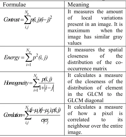
[image:3.612.314.522.297.522.2]In the original paper[16], 14 descriptors can be extracted from GLCM; many of these descriptors are highly correlated with each other [20]. The texture descriptors calculated from GLCM are contrast, energy, homogeneity and correlation of gray level values. Table 1 provides the equations and meaning for the four descriptors.
Table 1: Descriptors Calculated From The Normalized Co-occurrence Matrix And Its Meaning.
Formulae Meaning
2
g N
i,j
Contrast
p(i,j)(i j) It measures the amount of local variationspresent in an image. It is maximum when the image has similar gray values
2 1
g N
i
Energy p (i, j)
It measures the spatial closeness of the distribution of the co-occurrence matrix11
g N
i
p(i,j) Homogeneity
i j
It calculates a measure of the closeness of the distribution of element in the GLCM to the GLCM diagonalg N
i j
i j i,j
(i )(j ).p(i,j) Correlation
It calculates a measure of how a pixel is correlated to its neighbour over the entire image.where(.)is the standard deviation of the intensities of all reference pixels in the relationships that contributed to the GLCM, and
irepresents the horizontal mean andjrepresents the vertical mean in the GLCM4.2.Gray Level Run-Length Matrix
Instead of taking at pairs of pixels, the GLRLM looks at runs of pixels. A gray-level run is a set of consecutive and collinear pixel points having the same gray level value. The number of runs of pixels that have gray level i and length group j is represented by
r(i,j )
for α= 00, 450, 900, 1350
4062 image, a GLRLM r(i,j) is defined as the number of runs with pixels of gray level i and its run length j in four directions[17].
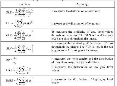
For a GLRLM, let M be the number of gray levels and N be the maximum run length. A set of descriptors can be extracted; many of these descriptors are irrelevant because they are highly correlated[21].
[image:4.612.115.503.213.500.2]In this work, seven textural descriptors are measured. from the GLRLM as shown in below Table 2 : short-run emphasis(SRE), long-runs emphasis(LRE), gray-level non uniformity(GLN), run-length non uniformity(RLN), run percentage(RP), low gray level run emphasis (LGRE), and high gray level run emphasis (HGRE)[22].
Table 2: Property and Formulas Descriptors Extracted From GLRLM
Formulae Meaning
2 1 1 1 SRE M N
r i j
r(i, j) n j
It measures the distribution of short runs.2 1 1 1 LRE M N
r i j r(i, j). j
n
It measures the distribution of long runs.2
1 1 1 M N
r i j
GLN r(i, j) n
It measures the similarity of gray level values throughout the image. The GLN is low if the gray levels are alike throughout the image.2
1 1 1 N M
r j i
RLN r(i, j) n
It measures the similarity of the length of runs throughout the image. The RLN is low if the run lengths are alike throughout the image.RP r
p
n n
It measures the homogeneity and the distribution of runs of an image in a given direction.
2 1 1 1 LGRE M N
r i j
r(i, j) n i
It measures the distribution of low gray level values2 1 1 1 HGRE M N
r i j r(i, j).i
n
It measures the distribution of high gray level valueswhere nris the total number of runs andnp is the number of pixels in the ROI.
In this work, we present a comparative study with two SML in the classification of digital mammography using two types of texture descriptors.
5. SUPERVISED MACHINE LEARNING
ALGORITHMS
Machine learning is a branch in artificial intelligence that can learn from data. It is based on building a model from training data that is used for making predictions or taking decisions.
The important property of machine learning algorithms is their distinctive ability to learn from input data make intelligent decisions[23]-[24].
Numerous SML techniques have been employed to resolve various classification problems and involve two phases namely training phase and testing phase [25].
In this work, supervised machine learning is used where the data are labeled. Any machine learning method uses a set of descriptors or features to characterise each object or image; these descriptors should be relevant.
Among SML techniques, SVMs would appear to be a good option because of their ability to discriminate in high-dimensional spaces. In addition, the appeal of SVMs is based on their strong connection to the underlying statistical learning and their strong theoretical foundations [25]. An important advantage of the SVM is that it is based on the principle of structural risk minimization [26].
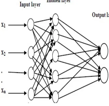
[image:4.612.116.501.214.501.2]4063 is mostly used. MLPs have been applied successfully to a wide range of information processing tasks, including pattern classification, function learning and time series prediction [27]. Among MLP performance one can distinguish data that is not linearly separable, or separable by a hyperplane.
In this paper, we have used SML like MLP and SVM algorithms for mammogram classification into benign and malignant using pattern texture. The performance of the classifiers has been evaluated using the accuracy
5.1.Multi-Layer Perceptron
Artificial neural networks have been created to separate the input instances into their correct classes. MLP proved useful when data is not linearly separable [28]. MLP is constructed on an input layer of nodes, followed by two or more layers of perceptron, the last of which is the output layer. The layers between the input layer and output layer are referred to as hidden layers with nonlinear activation functions [29].
[image:5.612.102.293.437.623.2]Practical applications for MLPs have been found in such diverse fields as speech recognition, image compression, medical diagnosis, autonomous vehicle control and financial prediction [30]. MLP architecture is represented in the form of figure1
Figure 1: The MLP architecture
In supervised classification, the number of the output layers is equal to the number of predefined classes.
The major aim of MLP algorithms is to automatically learn and make intelligent decisions. It is known as feed forward because it does not contain any cycles. And network output depends
only on the current input instance. Given the input and activation functions, MLP is defined by the current values of the weights. Learning consists in adapting the values of the weights to obtain the output.
The back-propagation learning employs a gradient descent method to train the network weights such that the Mean Squared Error(MSE) between the actual network output vectors and the desired output vectors is minimized [31].
The output is calculated and compared with the target output. The total MSE shown in Eq.1, is based on the training patterns of the calculated and target outputs
21 1
1
t o
2
m k
ij ij
j i
MSE
(1) where m is the number of examples in the trainingset, k is the number of output units,
t
ij is the target output value of the ith output unit for the jth trainingexample, and
o
ij is the actual real-valued output of the ith output unit for the jth training example.Usually a gradient descent algorithm was used to reduce the MSE between network output and the actual error rate in back-propagation algorithm. Once the network is trained it can be used to test new input data using the weights provided from the training test. The number of nodes in hidden layer will be adjusted in an attempt to achieve optimum classification accuracy.
5.2.Support Vector Machine
SVMs are invented by Vapnik in 1995; based on the statistical learning theory and risk minimisation. It has been applied for solving regression problems and binary classification [32].
Consider the training data
X
(x , y )
i i
ni1 wherex R
i
n, n is the number of training data,
1, 1
i
y
indicates the class ofx
i. When the decision function is not a linear function of the data, the data will be mapped from the input space into a high dimensional space by a nonlinear transformation called kernel function, defined as:
R
nR
d
where the decision hyperplane iscomputed. Kernels are a special class of function that allows inner products to be calculated directly in descriptor space [33].
4064 K exists, such that
K(x ,x )
i j
(x ). (x )
i
j . The decision function is defined as1
f(x)
n i.
i(x ,x )
i j ii
y K
w
(2)where
i are the weighting factors andw
idenotes the bias. After training, the condition
0
i
is valid for only a few examples, while for most
i
0
. Thus, the final decision function depends only on a small subset of the training vectors which are called support vectors. Finding the optimal hyperplane is equivalent to solve a quadratic optimisation problem [34].In the literature, there are several types of kernel such as polynomial, sigmoid, and radial basis function (RBF), Selecting the kernel K is very important for the performance of the classifier.
In this work, SVM is trained with the training samples using RBF formulated in Eq.3. It has the ability to transform the data into the higher dimension space without complicating computation since
is the unique parameter to be set2
2
(x , x ) exp
2
i j
i j
x x
K
(3)
where
x x
i
j is the Euclidian distance betweenx
i andx
j and
>0 is a constant that defines the kernel’s width and controls the flexibility of the kernel.In order to evaluate the performance of both classifiers (SVM and MLP) accuracy was adopted. Accuracy can be calculated from matrix confusion. Matrix confusion is a table with two rows and two columns that reports the number of false positive (FP), false negative (FN), true positive (TP), and true negative (TN)[35]. It allows visualisation of the performance of supervised learning algorithms like accuracy defined in Eq.4
TP TN
accuracy
TP TN FP FN
(4)The accuracy can be viewed as the ratio of the number of images correctly classified over the total number of test images. It is influenced by many factors. In this work, many parameters need to be optimised for getting a good accuracy.
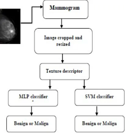
6. METHODOLOGY
The proposed work deals with an approach for extracting pattern texture in abnormal mammograms for classification into malignant or benign. The benchmark of the proposed method is a set of 40 mammograms: 20 mammogrames are selected from the Mini Mammographic Image Analysis Society (MIAS) database which is freely available over the Web[36]; and 20 mammogrames are produced by the National Institute of Oncology(NIO) Moulay Abdellah, of Mohammed V University in Rabat Morocco.
In this study, 22 mammographic images are benign and 18 mammographic images are malignant. The proposed method has been implemented in MATLAB environment
Figure 2 summarizes different stages of method developed in this work..
Figure 2: A general overview of the proposed method
6.1.Preprocessing
Preprocessing is necessary, firstly because we need to remove the unwanted parts in the background of mammogram such as artefact, and secondly all mammograms have various sizes.
[image:6.612.317.522.339.559.2]4065 experimental results in this paper, we converted all images into uniform 16 bit without affecting their quality.
[image:7.612.101.295.174.343.2]Original images are depicted in Fig.3 (a) and Fig.4 (a). Preprocessing result is shown in Fig.3 (b) and Fig.4 (b)
Figure. 3. Original mammogram (INO)(a), image cropped and resized (b)
Figure. 4. Original mammogram (mdb184)(a),, image cropped and resized (b)
Once the original image is cropped and resized, texture descriptors were extracted.
6.2.Texture Descriptors Extraction
In the current implementation, the descriptor is calculated using distance d=1, as reported in [37], where this parameter gave the best results. Moreover, four directions are taken into account in this work in order to give enough and reliable texture information.
For each ROI, each textural descriptor (e.g. contrast, correlation, etc.) was calculated 4 times (i.e. using 4 GLCMs). Each of these 4 GLCMs used a different orientation (0o, 45o, 90o, and 135o). In all
of these orientations we used the same distance d=1. The final value for the textural descriptor on a ROI was obtained averaging the values obtained from these 4 GLCMs. Finally, we concatenated
descriptors in one vector containing descriptors namely contrast, energy, homogeneity, and correlation.
In the same way, four GLRLMs according to the directions: 0o, 45o, 90o, and 135o are obtained and
seven textural descriptors are computed for each matrix. Besides, we calculated the average of these descriptors for all the directions for each ROI. Finally, we concatenated seven descriptors averaged: SRE, LRE, GLN, RLN, RP, LGRE, and HGRE in one vector
6.3.Data Representation and Arrangement
Overall a set of 11 descriptors for each ROI has been extracted and utilised in this research.
For each mammogram database (20 images from MIAS, and 20 images from NIO) the dataset used is composed of 20 instances distributed over two different classes: 9 malignant and 11 benign mammograms. Each instance is characterized by 11 numerical descriptors (7descriptors extracted from GRLM and 4 descriptors extracted from GLCM).
These descriptors, after being arranged in a file format suitable for each classifier, are used as input into a classifier to perform classification. The normalisation is needed in order to avoid the fact that descriptors in greater numeric ranges dominate those in smaller numeric ranges.
For each type of extracted descriptors, classification of mammograms into malignant or benign has been performed using MLP with 50 nodes using sigmoid activation function in the hidden layer in order to settle an architecture with a good accuracy. We divided the dataset as follows: 70% are assigned for training, 15% for validation, and 15% for testing.
MLP is trained to provide a value of 1 for a malignant and of 0 for benign mammograms. For SVM, yi=1 for benign and -1 for malignant
mammograms
7. EXPRIMENTAL RESULTS AND
DISCUSSION
In order to analyze the performance for various descriptors, the effectiveness of different texture descriptors extracted from GLCM and GRLM is evaluated and compared for each mammogram database and for each classifier.
In the case of GLCM descriptors, the input layer of the neural networks handles four descriptors extracted from the image. As mentioned in the previous subsection, two output layers denote
[image:7.612.102.291.180.499.2]4066 malignant or benign mammograms.
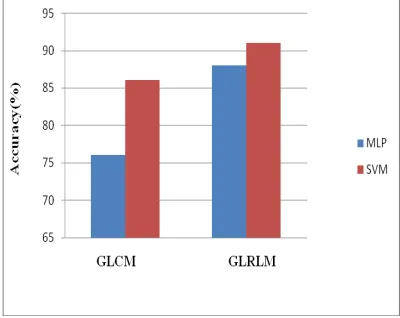
[image:8.612.90.300.99.444.2]Simulation runs have been performed using MLPs with 50 neurons in the hidden layer with a nonlinear sigmoid function as activation function in order to find the architecture with good accuracy. SVM classifier functions (svmtrain and svmclassify) are used to train and test data. In this work, 20% testing data are taken randomly from the training data, and RBF kernel used with σ=0.1. Figure 3 shows the comparison results of MLP with SVM algorithms when MIAS database is used and shows the comparison between GLCM and GLRLM.
[image:8.612.91.299.247.413.2]
Figure. 5. Comparison results with MIAS database
[image:8.612.99.299.545.704.2]As shown in Figure 5, the SVM algorithm has better classification accuracy compared to MLP for all texture descriptors. Texture descriptors derived from GLRM give the best accuracy (93%) compared to GLCM descriptors using both classifiers. The comparison result of MLP with SVM algorithms when NIO database is used is depicted in Figure 6
Figure. 6. Comparison results with NIO database
It can be noticed that using SVM as a classifier instead of MLP greatly improved the classification results for GRLM descriptors (91%). A better accuracy for both image databases is obtained with SVM classifier. The SVM algorithm achieves the highest accuracy compared with MLP algorithm. Figures 5 and Figure 6 reveal that pattern texture significantly improves the classification performance. The result shows that SVM is a consistent classifier for two used databases(MIAS and INO). A brief comparison of the proposed approach with the other approaches developed by researchers is presented in Table 3 in term of accuracy.
Table 3:Comparison of proposed system with other mammogram classification systems
Paper Year Database Accuracy
(%) Mavroforaks et
al.[10] 2006 83,9
Yuvaraj and
Ragupathy[12] 2013 MIAS 91,3
Lui et Tang[13] 2014 DDSM 94
Proposed
method 2017 MIAS INO 93 91
Since different researchers have used different mammography databases, different features and classifiers a precise comparison of outputs is a not a simple task. Though different data sets are employed in different methods, the reported performance is still an important standard to estimate the development and effectiveness of the proposed method. Among all these methods, our classification could obtain comparable performance with less complexity in feature extraction step in accuracy.
8. CONCLUSION
4067 and can be used as a second support for medical decision making.
The main limitation behind this study lies on the dataset where it tends to be relatively small data and does not contain important information. As a future research, examining a large data and other descriptors that contain a relevant information of breast lesions, and significantly contribute toward improving the classification accuracy.
AKNOWLDGMENT:
Our deep thanks to Pr. M. N. Boujida head of National Institute of Oncology(INO) Moulay Abdellah Rabat, Morocco, for helpful discussion and for providing the digitized mammogrames.
REFRENCES:
[1] D. B. Kopans. Breast Imaging. (Philadelphia, PA: J. B. Lippincoff, 1989.
[2] H. D. Cheng, X. J. Shi, R. Min, X. P. Cai and H. N. Du, “Automated detection of masses in mammogrames”, In C.H. Chen. and P.S.P. Wang (Eds.), Handbook of pattern recognition and computer vision, 3rd Edition World Scientific, 2005, pp.303-323.
[3] S. V. Destounis, P. DiNitto, W. Logan-Young, E. Bonaccio, M. L. Zuley, and K. M. Willison, “Can computer-aided detection with double reading of screening mammograms help decrease the false-negative rate? Initial experience,” Radiology, vol. 232, N.2,2004, pp. 578–584.
[4] M.Khuzi, R. Besar, W.Zaki, and NN. Ahmad, “Identification of masses in digital mammogram using gray level co-occurrence matrices”,
Biomedical Imaging and Intervention Journal. 2009,Vol.5.No.3:e17
[5] Y. Ben Youssef, E. Abdelmounim., and A. Belaguid,“Mammogram classification using support vector machine”. In handbook of researcher on advanced trends in microwave and communication engineering, IGI Global ed. 2017, pp .587-614
[6] Y.Q. Chen, M.S. Nixon and D. W. Thomas, Statistical geometrical features for texture classification, Pattern Recognition,Vol.2,No.4, pp.537-552.
[7] S.A.Karkanis, G.D.Magoulas, D.Iakovidis, D.E.Maroulisand, and M. O. Schurr, “On the importance of feature descriptors for the characterization of Texture”, In 4th World
Multi-conference on Systems, Cybernetics and Informatics, 2000, pp.1–6.
[8] M.Tuceryan and A. K. Jain, “Texture Analysis”
in the Handbook of Pattern Recognition and Computer Vision (2nd Edition), by C. H. Chen, L. F. Pau, and P. S. P. Wang (eds.), World Scientific Publishing Co., 1998, pp.207-248. [9] Y.BenYoussef, E. Abdelmounim, J. Zbitou,
A.Errkik, and A. Belaguid, “Malignant Mammogram Classification using Artificial neural network”, in Proceedings of the 2nd Workshop on Advanced Signal Processing and Information Technology. AspiT’2016,pp.56-59. [10]M.E.Mavroforakis,H.V.Georgiou,D.Dimitopoulo
s,D.Cavouras, and S. Theodoridis,“
Mammographic masses characterization based on localized texture and data set fractal analysis using linear, neural and support vector machine classifiers”,
Artif.Intell.Med,Vol.37,N.2,2006,pp145–162.
[11] K.Ganesan, U.R.Acharya, C.K.Chua, L.C.Min, T.Abraham and K.H.Ng. “Computer aided breast cancer detection using mammograms: A Review”, IEEE reviews in biomedical
engineering, vol.6, 2013, pp.77-98.
[12] K. Yuvaraj and U. S. Ragupathy, “Computer aided segmentation and classification of mass in
mammographic images using
ANFIS”.,European Journal of Biomedical Informatics 9, 37, 2013,pp.37-41.
[13] X. Liu, and J. Tang, “Mass classification in mammograms using selected geometry and texture features, and a new SVM-based feature selection method”, IEEE Syst. Jour. Vol.8, N.3,2014, pp.910–920.
[14] S. Y. Lu and K. S. Fu, “A syntactic approach to texture analysis”, Computer Graphics and
Image Proc. Vol.7, 1978, pp.303-330.
[15] M. Hassner and J. Sklansky, “ The use of Markov random fields as models of texture”,
Computer Graphics Image Proc., 1980,.12, pp.357-370.
[16] R.M. Haralick, K. Shanmugam, and I. Dinstein, “Textural features for image classification”
IEEE Trans. Syst. Man Cybernetics,Vol.3, 1973,pp.610-621.
[17] M.M. Galloway, “Texture classification using gray level run length” Comput.Graphics Image Process. Vol.4, 1975, pp. 172–179.
4068 [19] Haralick, R.M., and L.G. Shapiro. “Computer
and Robot Vision”., Vol. 1, Addison-Wesley, 1992.
[20] A. Baraldi, F. Parmiggiani, “An investigation of the textural characteristics associated with gray level co-occurrence matrix statistical parameters”, IEEE Transactions on Geoscience and Remote Sensing,Vol.33.No.2.1995,pp.293– 304.
[21] X.Tang, “Dominant Run-Length Method for Image Classification”, Technical Report
,Woods Hole Oceanog. Inst. Jul,1997.
[22] A. Chu, C.M. Sehgal and J. F. Greenleaf, “Use of gray value distribution of run lengths for texture analysis”, Pattern Recognition Letters,
Vol.11.1990, pp. 415-420.
[23] E.Alpaydin, “Introduction to machine learning”, 3rded. Cambridge, 2014, MA The MIT Press.
[24] C.M.Bishop, “Pattern recognition and machine learning” ,2006, New York Springer.
[25] S. Kotsiantis, I. Zaharakis and P. Pintelas, “Machine learning: a review of classification and combining techniques”, Artificial Intelligence Review,Vol.26, No.3, 2006, pp. 159-190.
[26] V.Vapnik, “The Nature of Statistical Learning Theory”, 1995, Springer, New York.
[27] P.J.G. Lisboa. “Neural Networks: Current Applications”,1992, Chapman & Hall, London. [28] G.P. Zhang, “Neural networks for classification:
a survey”, IEEE Trans Syst Man Cy,Part C, 2000, Vol.30,No.4, pp.451-462.
[29] A.K.Jain, J.Mao, and K.M. Mohiudden, “Artificial Neural Networks: A Tutorial”, IEEE computer, special issue on neural computing,Vol.29, No.3, 1996, pp.31-44. [30] A.J. Shepherd, “Second order Methods for
Neural Networks, Fast and Reliable Training Methods for Multi-Layer Perceptrons”, 1997,Springer-Verlag London.
[31] D.E.Rumelhart, G.E. Hinton, and R.J. Williams, “Learning internal representations by error propagation”, Nature, Vol.323, 1986, pp.533-536.
[32] C. J. Burges, “A tutorial on support vector machines for pattern recognition”, Data Mining and Knowledge Discovery, vol.2, 1998,pp.121-167.
[33] C.Campbell, “An introduction to kernel methods”. In R.J. Howlett and L.C. Jain (Ed.), Radial Basis Function Networks: Design and Applications, 2000, page155-192. Springer-Verlag, Berlin.
[34] G.P. Gill, and W. Murray, “The Computation of Lagrange multiplier estimates for constrained minimization”, Math.prog,Vol.17,No.1,1979 pp.32-60.
[35] C. Metz, “ROC Methodology in Radiologic Imaging”, Investigative radiology, Vol. 21, 1986,pp. 720-733.
[36] J.Suckling, et al. “The Mammographic Image Analysis Society Digital Mammogram Database(MIAS) ”, Proceedings of the 2nd
Workshop on Digital Mammography, 1994,pp. 375-378.