Language Identification in Code-Switching Scenario
Naman Jain
LTRC, IIIT-H, Hyderabad, India [email protected]
Riyaz Ahmad Bhat LTRC, IIIT-H, Hyderabad, India [email protected]
Abstract
This paper describes a CRF based token level language identification system en-try to Language Identification in Code-Switched (CS) Data task of CodeSwitch 2014. Our system hinges on using con-ditional posterior probabilities for the in-dividual codes (words) in code-switched data to solve the language identification task. We also experiment with other lin-guistically motivated language specific as well as generic features to train the CRF based sequence labeling algorithm achiev-ing reasonable results.
1 Introduction
This paper describes our participation in the Lan-guage Identification in Code-Switched Data task at CodeSwitch 2014 (Solorio et al., 2014). The workshop focuses on NLP approaches for the analysis and processing of mixed-language data with a focus on intra sentential code-switching, while the shared task focuses on the identifica-tion of the language of each word in a code-switched data, which is a prerequisite for ana-lyzing/processing such data. Code-switching is a sociolinguistics phenomenon, where multilingual speakers switch back and forth between two or more common languages or language-varieties, in the context of a single written or spoken conversation. Natural language analysis of code-switched (henceforth CS) data for various NLP tasks like Parsing, Machine Translation (MT), Au-tomatic Speech Recognition (ASR), Information Retrieval (IR) and Extraction (IE) and Semantic Processing, is more complex than monolingual data. Traditional NLP techniques perform miser-ably when processing mixed language data. The performance degrades at a rate proportional to the amount and level of code-switching present in the
data. Therefore, in order to process such data, a separate language identification component is needed, to first identify the language of individual words.
Language identification in code-switched data can be thought of as a sub-task of a document level language identification task. The latter aims to identify the language a given document is writ-ten in (Baldwin and Lui, 2010), while the former addresses the same problem, however at the token level. Although, both the problems have separate goals, they can fundamentally be modeled with a similar set of features and techniques. However, language identification at the word level is more challenging than a typical document level lan-guage identification problem. The number of fea-tures available at document level is much higher than at word level. The available features for word level identification are word morphology, syllable structure and phonemic (letter) inventory of the language(s). Since these features are related to the structure of a word, letter based n-gram models have been reported to give reasonably accurate and comparable results (Dunning, 1994; Elfardy and Diab, 2012; King and Abney, 2013; Nguyen and Dogruoz, 2014; Lui et al., 2014). In this work, we present a token level language identification sys-tem which mainly hinges on the posterior prob-abilities computed using n-gram based language models.
The rest of the paper is organized as follows: In Section 2, we discuss about the data of the shared task. In Section 3, we discuss the methodology we adapted to address the problem of language identification, in detail. Experiments based on our methodology are discussed in Section 4. In Sec-tion 5, we present the results obtained, with a brief discussion. Finally we conclude in Section 6 with some future directions.
2 Data
TheLanguage Identification in the Code-Switched (CS) data shared task is meant for language identification in 4 language pairs (henceforth LP) namely, Nepali-English (N-E), Spanish-English(S-E),Mandarin-English(M-E) and Mod-ern Standard Arabic-Arabic dialects(MSA-A). So as to get familiar with the training and testing data, trial data sets consisting of20tweets each, corsponding to all the language-pairs, were first re-leased. Additional test data as “surprise genre” for
S-E, N-E and MSA-A were also released, which comprised of data from Facebook, blogs and Ara-bic commentaries.
2.1 Tag Description
Each word in the training data is classified into one of the 6 different classes which are, Lang1, Lang2, Mixed, Other, Ambiguous and NE. “Lang1” and “Lang2” tags correspond to words specific to the languages in an LP. “Mixed” words are those words that are partially in both the lan-guages. “Ambiguous” words are the ones that could belong to either of the language. All gib-berish and unintelligible words and words that do not belong to any of the languages fall under “Other” category. “Named Entities” (NE) com-prise of proper names that refer to people, places, organizations, locations, movie titles and song ti-tles etc.
2.2 Data Format and Data Crawling
Due to Twitter policies, distributing the data di-rectly is not possible in the shared task and thus the trial, training and testing data are provided as char offsets with label information along with tweetID1
and userID2. We usetwitter3python script to crawl
the tweets and our own python script to further to-kenize and synchronize the tags in the data.
Since the data for “surprise genre” comes from different social media sources, the ID format varies from file to file but all the other details are kept as is. In addition to the details, the tokens ref-erenced by the offsets are provided unlike Twitter data. (1) and (2) below, show the format of tweets in train and test data respectively, while (3) shows a typical tweet in the surprise genre data.
1Each tweet on Twitter has a unique tweetID 2Each user on Twitter carries a userID
3http://emnlp2014.org/workshops/CodeSwitch/scripts/ twitter.zip
(1) TweetID UserID startIndex endIndex Tag
(2) TweetID UserID startIndex endIndex
(3) SocialMediaID UserID startIndex endIn-dex Word
2.3 Data Statistics
The CS data is divided into two types of tweets (henceforth posts)4namely, Code-switched
posts and Monolingual posts. Table 1 shows the original number of posts that are released for the shared task for all LPs, along with their tag counts. Due to the dynamic nature of social media, the posts can be either deleted or updated and thus different participants would have crawled different number of posts. Thus, to come up with a compa-rable platform for all the teams, the intersection of data from all the users is used as final testing data to report the results. Table 1 shows the number of tweets or posts in testing data that are finally used for the evaluation.
3 Methodology
We divided the language identification task into a pipeline of 3sub-tasks namely Pre-Processing,
Language Modeling, andSequence labeling using CRF5. The pipeline is followed for all the LPs with
some LP specific variations in selecting the most relevant features to boost the results.
3.1 Pre-Processing
In the pre-processing stage, we crawl the tweets from Twitter given their offsets in the training data and then tokenize and synchronize the words with their tags as mentioned in Section 2.2. For each LP we separate out the tokens into six classes to use the data for Language Modeling and also to manually analyze the language specific properties to be used as features further in sequence labeling . While synchronizing the words in a tweet with their tags, we observed that some offsets do not match with the words and this would lead to mis-match of labels with tokens and thus degrade the quality of training data.
To filter out the incorrect instances from the training data, we frame pattern matching rules which are specific to the languages present. But this filtering is done only for the words present in 4In case of twitter data, we have tweets but in case of sur-prise genre data we have posts
Language Pairs # Tweets # Tokens
CodeSwitched Monolingual Ambiguous Lang1 Lang2 Mixed NE Other
Train
MSA-A dialects 774 5,065 1,066 79,134 16,291 15 14,112 8,699
Mandarin-English 521 478 0 12,114 2,431 12 1,847 1,025
Nepali-English 7,203 2,790 126 45,483 60,697 117 3982 35,651 Spanish-English 3,063 8,337 344 77,107 33,099 51 2,918 27,227
Test
MSA-A dialects I 32 2,300 11 44,314 141 0 5,939 3,902
Mandarin-English 247 66 0 4,703 881 1 254 442
Nepali-English 2,665 209 0 12,286 17,216 60 1,071 9,635
Spanish-English 471 1,155 43 7,040 5,549 12 464 4,311
MSA-A dialects II 293 1,484 119 10,459 14,800 2 4,321 2,940
Sur
prise MSA-A dialectsNepali-English 20- 82- 1100 2,687173 6,930699 03 1,097127 1,19088
[image:3.595.307.529.277.379.2]Spanish-English 22 27 1 636 306 1 38 120
Table 1: Data Statistics
‘Lang1’ and ‘Lang2’ classes. There are two rea-sons to consider these labels. First, ‘Lang1’ and ‘Lang2’ classes hold maximum share of words in any LP as shown in Table 1, and thus have a higher impact on the overall accuracy of the language identification system. In addition to the above, these categories correspond to the focus point of the shared task. Second, for ‘Ambiguous’, ‘NE’ and ‘Other’ categories, it is difficult to find the patterns according to their definitions. Although rules can be framed for ‘Mixed’ category, since their count is too less as compared to the other categories (Table 1), it is of no use to train a sepa-rate language model with very less number of in-stances.
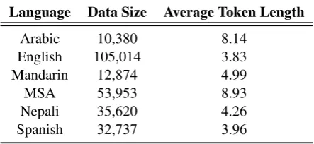
For Mandarin and Arabic data sets, any word present in Roman script is excluded from the data. Similarly for English and Nepali, if any word con-tains characters other than Roman or numeral they are excluded from the data. In addition to the rule for English and Nepali, the additional alpha-bets in Spanish are also included in the set of Ro-man and numeral entries. Table 2 shows the num-ber of words that remained in each of the lan-guages/dialects, after the preprocessing.
One of the bonus points in the shared task is that 3 out of 4 LPs share ‘English’ as their sec-ond language. In order to increase the training size for English, we merged all the English words into a single file and thus reduced the number of lan-guage models to be trained from 8 to 6, one for each language (or dialect).
Language Data Size Average Token Length
Arabic 10,380 8.14
English 105,014 3.83
Mandarin 12,874 4.99
MSA 53,953 8.93
Nepali 35,620 4.26
Spanish 32,737 3.96
Table 2: Data Statistics after Filtering
3.2 Language Modeling
In this stage, we train separate smoothed n-gram based language models for each language in an LP. We compute the conditional probability for each word using these language models, which is then used as a feature, among others for sequence la-beling to finally predict the tags.
3.2.1 N-gram Language Models
Given a wordw, we compute the conditional prob-ability corresponding to k6classes c
1, c2, ... , ck
as:
p(ci|w) = p(w|ci)∗p(ci) (1)
The prior distribution p(c) of a class is es-timated from the respective training sets shown in Table 2. Each training set is used to train a separate letter-based language model to estimate the probability of word w. The language model p(w) is implemented as an n-gram model using the IRSTLM-Toolkit (Federico et al., 2008) with Kneser-Ney smoothing. The language model is
defined as:
p(w) =Yn
i=1
p(li|li−i−k1) (2)
wherelis a letter andkis a parameter indicating the amount of context used (e.g., k=4 means 5-gram model).
3.3 CRF based Sequence Labeling
After Language Modeling, we use CRF-based (Conditional Random Fields (Lafferty et al., 2001)) sequence labeling to predict the labels of words in their surrounding context. The CRF algo-rithm predicts the class of a word in its surround-ing context taksurround-ing into account other features not explicitly represented in its structure.
3.3.1 Feature Set
In order to train CRF models, we define a feature set which is a hybrid combination of three sub-types of features namely, Language Model Fea-tures (LMF), Language Specific FeaFea-tures (LSF) and Morphological Features (MF).
LMF: This sub-feature set consists of poste-rior probability scores calculated using language models for each language in an LP. Although we trained language models only for ‘Lang1’ and ‘Lang2’ classes, we computed the probabil-ity scores for all the words belonging to any of the categories.
LSF: Each language carries some specific traits that could assist in language identification. In this sub-feature set we exploited some of the lan-guage specific features exclusively based on the description of the tags provided. The common fea-tures for all the LPs are HAS NUM (Numeral is present in the word),HAS PUNC(Punctuation is present in the word),IS NUM(Word is a numeral),
IS PUNC(word is a punctuation or a collection of punctuations), STARTS NUM (word starts with a numeral) andSTARTS PUNC (word starts with a punctuation). All these features are used to gener-ate variations to distinguish ‘Other’ class from rest of the classes during prediction.
Two features exclusively used for the English sharing LPs areHAS CAPITAL(capital letters are present in the word) andIS ENGLISH (word be-longs to English or not). HAS CAPITAL is used to capture the capitalization property of the En-glish writing system. This feature is expected to
help in the identification of ‘NEs’.IS ENGLISHis used to indicate whether a word is an valid English word or not, based on its presence in English dic-tionaries. We used dictionaries available in PyEn-chant7.
For the M-E LP, we are using ‘TYPE’8 as a
feature with possible values as ENGLISH, MAN-DARIN, NUM, PUNC and OTHER. If all the characters in the word are English alphabets EN-GLISH is taken as the value and Mandarin oth-erwise. Similar checks are used for NUM and PUNC types. But if no case is satisfied, OTHER is taken as the value.
We observed that the above features did not con-tribute much to distinguish between any of the tags in case of theMSA-A LP. Since this pair consists of two different dialects of a language rather than two different languages, the posterior probabilities would be close to each other as compared to other LPs. Thus we use the difference of these probabil-ities as a feature in order to discriminate ambigu-ous words or NEs that are spelled similarly. MF: This sub-feature set comprises of the mor-phological features corresponding to a word. We automatically extracted these features using a python script. The first feature of this set is a bi-nary length variable (MORE/LESS) depending on the length of the word with threshold value4. The other8features capture the prefix and suffix prop-erties of a word,4 for each type. In prefix type,
4,3,2and1characters, if present, are taken from the beginning of a word as 4 features. Similarly for the suffix type,1,2,3and4characters, again if present, are taken from the end of a word as4
features. In both the cases if any value is miss-ing, it is kept as NULL (LL). (4) below, shows a typical example from English data with the MF sub-feature set for the word ‘one’, where F1 rep-resents the value of binary length variable, F2-F5 and F6-F9 represent the prefix and suffix features respectively.
(4) one
WordLessF1 LLF2 oneF3 onF4oF5LLF6 oneF7 neF8eF9 3.3.2 Context Window
Along with the above mentioned features, we chose an optimal context template to train the CRF 7PyEnchant is a spell checking library in Python (http://pythonhosted.org/pyenchant/)
models. We selected the window size to be5, with
2words before and after the target word. Furnish-ing the trainFurnish-ing, testFurnish-ing and surprise genre data with the features discussed in 3.3.1, we trained4
CRF models on training data using feature tem-plates based on the context decided. These mod-els are used to finally predict the tags on the testing and surprise genre data.
4 Experiments
The pipeline mentioned in Section 3 was used for the language identification task for all the LPs. We carried out a series of experiments with pre-processing to clean the training data and also to synchronize the testing data. We also did some post-processing to handle language and tag spe-cific cases.
In order to generate language model scores, we trained 6language models (one for each lan-guage/dialect) on the filtered-out training data as mentioned in Table 2. We experimented with dif-ferent values of n-gram to select the optimal value based on the F1-measure. Table 3 shows the opti-mal order of n-gram, selected corresponding to the highest value ofF1-score. Using the optimal value of n-gram, language models have been trained and then posterior probabilities have been calculated using equation (1).
Finally, we trained separate CRF models for each LP, using theCRF++9tool kit based on the
features described in Section 3.3.1 and the feature template in Section 3.3.2. To empirically find the relevance of features we also performed leave-one out experiments so as to decide the optimal fea-tures for the language identification task (more de-tails in Section 4.1). Then, using these CRF mod-els, tags were predicted on the testing and surprise genre datasets.
Language-Pair N-gram
MSA-A 5
M-E 5
N-E 6
S-E 5
Table 3: Optimal Value of N-gram 4.1 Feature Ranking
We expect that some features would be more im-portant than others and would impact the task 9http://crfpp.googlecode.com/svn/trunk/doc/index.html? source=navbar
of language identification irrespective of the lan-guage pair. In order to identify such optimal fea-tures for the language identification task, we rank them based on their information gain scores. 4.1.1 Information Gain
We used information gain to score features ac-cording to their expected usefulness for the task at hand. Information gain is an information theoretic concept that measures the amount of knowledge that is gained about a given class by having access to a particular feature. Iff is the occurrence an individual feature and f¯the non-occurrence of a feature, information gain can be measured by the following formula:
G(x) =P(f)XP(y|f)logP(y|f)
+P( ¯f)XlogP(y|f¯)logP(y|f¯) (3)
For each language pair, the importance of fea-ture types are represented by the following order:
• MSA-A dialects:token>word morphology >posterior probabilities>others
• Mandarin-English:token>posterior prob-abilities > word morphology > language type>others
• Nepali-English:token>posterior probabil-ities>word morphology>dictionary> oth-ers
• Spanish-English: token > posterior proba-bilities>word morphology>others> dic-tionary
Apart from MSA-A dialects, top 3 features sug-gested by information gain are token and its sur-rounding context, posterior probabilities and word morphology. For Arabic dialects word morphol-ogy is more important than posterior probabilities. It could be due to the fact that Arabic dialects share a similar phonetic inventory and thus have similar posterior probabilities. However, they differ sig-nificantly in their morphological structure (Zaidan and Callison-Burch, 2013).
Token Level
Language Pairs Ambiguous Lang1 Lang2 Mixed NE Other
R P F1 R P F1 R P F1 R P F1 R P F1 R P F1 Overall Accuracy
Test
MSA-A I 0.00 0.00 0.00 0.92 0.95 0.94 0.40 0.03 0.06 - - - 0.70 0.77 0.73 0.90 0.85 0.87 0.90 M-E - - - 0.98 0.98 0.98 0.67 0.66 0.67 0.00 1.00 0.00 0.84 0.38 0.53 0.22 0.71 0.33 0.88 N-E - - - 0.95 0.93 0.94 0.98 0.96 0.97 0.00 1.00 0.00 0.39 0.79 0.52 0.94 0.96 0.95 0.95 S-E 0.00 1.00 0.00 0.88 0.81 0.84 0.83 0.90 0.86 0.00 1.00 0.00 0.16 0.40 0.23 0.83 0.80 0.82 0.83 MSA-A II 0.00 0.00 0.00 0.91 0.47 0.62 0.36 0.84 0.51 0.00 1.00 0.00 0.59 0.80 0.68 0.80 0.71 0.75 0.60
Sur
prise MSA-AN-E 0.00 0.00 0.00 0.94 0.38 0.54 0.46 0.93 0.61 0.00 1.00 0.00 0.52 0.78 0.62 0.96 0.96 0.96- - - 0.92 0.76 0.84 0.95 0.89 0.91 - - - 0.35 0.92 0.50 0.85 0.89 0.87 0.620.86 S-E 0.00 1.00 0.00 0.86 0.81 0.83 0.82 0.87 0.85 0.00 1.00 0.00 0.15 0.40 0.22 0.82 0.78 0.80 0.94
Table 4: Token Level Results
Left Out Feature MSA-A M-E N-E S-E Context 76.32 94.07 93.97 92.30 Morphology 79.29 93.67 93.98 93.51 Probability 79.24 89.16 93.86 93.28 Dictionary - 87.75 93.73 92.99
Language Type - 87.97 -
[image:6.595.104.496.66.164.2]-Others 78.80 83.84 92.10 92.20 All Features 79.37 95.11 94.52 93.54
Table 5: Leave-one-out Experiments
5 Results and Discussion
Each language identification system is evaluated against two data tracks namely, ‘Testing’ and ‘prise Genre’ data as mentioned in Section 2. Sur-prise genre data of Mandarin-English LP was not provided, so no results are available. All the results are provided on two levels, comment/post/tweet and token level. Tables 4 and 6 show results of our language identification system on both the levels respectively.
In case of Tweets, systems are evaluated using the following measures: Accuracy,Recall, Preci-sion and F-Score. However at token level, sys-tems are evaluated separately for each tag in an LP using Recall, Precision and F1-Score as the measures. Table 4 shows that the results for ‘Am-biguous’ and ‘Mixed’ categories are either miss-ing (due to absence of tokens in that category), or have0.00F1-Score. One obvious reason could be the sparsity of data for these categories.
6 Conclusion and Future Work
In this paper, we have described a CRF based to-ken level language identification system that uses a set of naive easily computable features guarantee-ing reasonable accuracies over multiple language pairs. Our analysis showed that the most important
Language Pairs Tweet Level
Accuracy Recall Precision F-score
Test
MSA-A I 0.605 0.719 0.025 0.048 M-E 0.751 0.814 0.863 0.838 N-E 0.948 0.979 0.966 0.972 S-E 0.835 0.773 0.692 0.730 MSA-A II 0.469 0.823 0.213 0.338
Sur
[image:6.595.73.283.206.338.2]prise MSA-AN-E 0.4570.735 0.8330.900 0.1280.419 0.2220.571 S-E 0.830 0.765 0.689 0.725
Table 6: Comment/Post/Tweet Level Results
feature is the word structure which in our system is captured by n-gram posterior probabilities and word morphology. Our analysis of Arabic dialects shows that word morphology plays an important role in the identification of mixed codes of closely related languages.
7 Acknowledgement
We would like to thank Himani Chaudhry for her valuable comments and suggestions that helped us to improve the quality of the paper.
References
Timothy Baldwin and Marco Lui. 2010. Language identification: The long and the short of the mat-ter. In Human Language Technologies: The 2010 Annual Conference of the North American Chap-ter of the Association for Computational Linguistics, pages 229–237. Association for Computational Lin-guistics.
Ted Dunning. 1994. Statistical identification of lan-guage. Computing Research Laboratory, New Mex-ico State University.
Heba Elfardy and Mona T Diab. 2012. Token level identification of linguistic code switching. In COL-ING (Posters), pages 287–296.
han-dling large scale language models. InInterspeech, pages 1618–1621.
Ben King and Steven P Abney. 2013. Labeling the languages of words in mixed-language documents using weakly supervised methods. InHLT-NAACL, pages 1110–1119.
John Lafferty, Andrew McCallum, and Fernando CN Pereira. 2001. Conditional random fields: Prob-abilistic models for segmenting and labeling se-quence data. In Proceedings of the International Conference on Machine Learning, pages 282–289. Marco Lui, Jey Han Lau, and Timothy Baldwin. 2014.
Automatic detection and language identification of multilingual documents. volume 2, pages 27–40. Dong Nguyen and A Seza Dogruoz. 2014. Word
level language identification in online multilingual communication. In Proceedings of the 2013 Con-ference on Empirical Methods in Natural Language Processing.
Thamar Solorio, Elizabeth Blair, Suraj Maharjan, Steve Bethard, Mona Diab, Mahmoud Gonheim, Abdelati Hawwari, Fahad AlGhamdi, Julia Hirshberg, Alison Chang, and Pascale Fung. 2014. Overview for the first shared task on language identification in code-switched data. InProceedings of the First Workshop on Computational Approaches to Code-Switching. EMNLP 2014, Conference on Empirical Methods in Natural Language Processing, Octobe, 2014, Doha, Qatar.