A New Algorithm to Provide all Solutions of SSP Problem

(1)

20

A New Algorithm to Provide all Solutions of SSP

Problem

Vishal Kesri

Tek Infotree Pvt Ltd New Delhi, India

ABSTRACT

Sum of subset (SSP) is an important problem of complexity theory and cryptography in computer science. The SSP involves searching from a given set of distinct integers to find all the subsets whose sum of elements equal to certain integer capacity. The importance of this algorithm is that, it can be applied to create a better decryption technique and in many others. The proposed algorithm is able to find all solutions of SSP from a given set of integers. Simulation shows that the algorithm takes less number of steps as compared to traditional back tracking algorithm.

General Terms

NP hard, NP complete, cryptography, encryption, decryption.

Keywords

Search, Total, Next Element, Next Search, Set-A, Set-B, Remain-Set, Final Matrix.

1. INTRODUCTION

The Subset-Sum Problem (SSP) is one the most fundamental NP-complete problems [2] and simple of its kind. Given a set of n data items with positive weights and a given capacity, SSP is use to find out all the subset whose sum is equal to given capacity. SSP is useful in solving many real life problems that includes, decision version of SSP with unique solutions represent a secret message in a SSP-based cryptosystem [1]. It is also applicable in combinatorial problem [8], scheduling problem [11], 0-1 integer problem [10] and bin packing algorithm [9]. The Subset-Sum Problem is often thought of as a special case of the Knapsack Problem, where the weight of a data item is proportional to its size. Therefore, algorithms for the Knapsack Problem can be applied for SSP automatically.

1.1 Brief History

There exists some algorithms which provide the solution of SSP but the time complexity of these algorithms is very high. A naive algorithm solves the SSP in O(n2n), as the algorithm finds all possible subsets and evaluates them to obtain the solution.

An improved algorithm suggested by Horowitz and Sahni in 1974, achieves the solutions in time O(n2n/2)and the exact algorithm for solving this have not been improved since then [1]. Some dynamic programming algorithms give faster solutions to a special case of SSP, where the capacity is relatively small and many other algorithms have been proposed under different heuristics [7].

2. DEFINITION

Given an instance S = {x1, x2, . . . , xn} of SSP, is a set of n distinct positive numbers such that, to find all combinations of this numbers (usual called subset) whose sum is equal to some integer capacity ‘C’. Where set S is the input vector, containing x1, x2, . . . , xn are the data elements and ‘C’ is the given capacity. The desire solutions can be expressed by either a fixed or variable sized vector. Here, in this paper variable sized solution vector is used.

2.1 Mathematical Definition

Given the input vector, x1…….xn taken in ascending order and a capacity C such that

, where xi >0 and 1 ≤ i ≤ n ……….(1)

, where yi = 1...……….(2)

x1 ≤ C……….………(3)

2.2 Notations

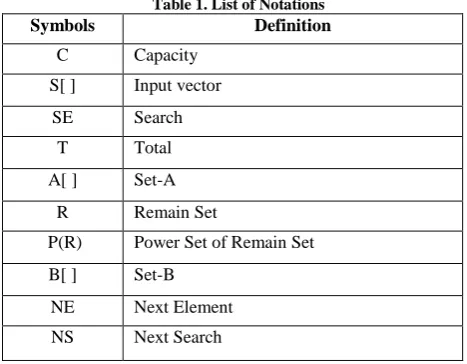
[image:1.595.309.543.441.623.2]

The notations used in this algorithm are given in table 1.

Table 1. List of Notations

Symbols Definition

C Capacity

S[ ] Input vector

SE Search

T Total

A[ ] Set-A

R Remain Set

P(R) Power Set of Remain Set

B[ ] Set-B

NE Next Element

NS Next Search

Search: Initially search value is equal to the capacity. However, at each recursion step the capacity value is re calculated and assign to SE.

(2)

21 Algorithm for ‘Total’

/* n= Size of input array S[ ] */ /* calculate1 is a variable */ for (i = 0; i < n; i++) {

calculate1 = calculate1 + S[i]; if ( calculate1 ≤ SE)

{

T = calculate1; }

else break; }

Algorithm 1

Set-A: the set-A contains the data elements of set S whose summation must be less than or equal to SE and assigned to T.

Algorithm for ‘Set-A’

/* n= Size of input array S[ ] */ /* calculate2 is a variable */

for (i = 0; i < n; i++) {

calculate2 = calculate2 + S[i]; if ( calculate2 ≤ SE)

{

A[i] = S[i]; }

else break; }

Algorithm 2

Remain Set: Remain set contains the elements whose individual element are less than or equal to SE.

Algorithm for ‘Remain-Set’

/* n= Size of input array S[ ] */ /* Capacity = Entered by the user */

for (i = 0; i < n; i++) {

calculate3 = calculate3 + S[i]; j = i;

if ( calculate3 ≥ SE) break;

}

for (i = j; i < n; i++) {

if ( S[i] ≤ capacity) {

R[i] = S[i]; }

else break; }

Algorithm 3

R' is a power set of R, which contains subsets of R. the summation of the elements in individual subset is less than or equal to SE. xi is the subset of R

Example

R= {2, 3, 5, 7 } SE = {8}

R' = {(2), (3), (5), (7), (2, 3), (2, 5), (3, 5)}

Here we not consider (3, 7), etc. as element of R' because the value of (3, 7) become 10 after add “3+7”, which is ≥’SE’.

Set-B: In each iteration, Set-B contains one element of R' and in the second iteration, Set-B contains second element and so on.

Algorithm for ‘Set-B’

mlength of R'[ ]

for  1 to m

do BR' [ ] /* Here pass one by one each

element of R' into B */

Algorithm 4

Next Element: the NE contains the summation of all the element of the Set-B for a particular iteration.

Next Search: NS contains a value that becomes the capacity for the next level. That is NS become the value of SE for next level.

Final Matrix: The final matrix is important to calculate the solutions of SSP. When T = = SE we get a solution of SSP. Final Matrix has three columns (Level, Set-A, Set-B) and n rows where “n=number of levels”.

Solution: The element, which appear odd number of time in the final matrix, that become a solution of SSP.

2.3 Algorithm

The propose algorithm describe below in Algorithm-5: Algorithm for ‘SSP’

/* S [ ], is an input array, B[ ] is an array of Set-B Initial flag=1, flag2=1 */

void main {

read S , C ; SSP (C); }

(3)

22 {

Step-1:

if S[0] > ‘SE’ && level == 1 exit ;

else if S[0] > ‘SE’

return previous level at step-5 else

continue ; Step-2:

calculate A [] calculate ‘T’

Step-3:

if flag2 == 0 {

calculate R with “<” condition flag2 = 1;

} if flag ≠ 0

calculate R with “≤” condition calculate R'

Step-4:

if ‘T’= = ‘SE’ {

if R' = = null && level = = 1 {

flag = 0; Solution ( ) ; }

else {

flag = 1; Solution ( ) ; }

} Step-5:

if R'= = null && level = = 1 exit;

if R'= = null && level ≠ 1 return previous level at step-5; else

send one by one each element to Set-B from R'

Step-6:

calculate NE calculate NS

if B[0] = = NE = = NS flag2 = 0; SSP ( NS );

/* NS become SE value for next level */

Solution ()

{ Step-7:

calculate Final Matrix

Step-8:

calculate solution if flag = = 0 exit;

else if flag = = 1 return ; }

Algorithm 5

3. ANALYSIS OF ALGORITHM

The space complexity of this algorithm is:

Time complexity need to be calculate during future work.

3.1 Comparison

[image:3.595.319.540.270.405.2]

The Figure-1 shows a comparison between the traditional backtracking algorithms and propose algorithm. This comparison done by taking a fixed input sequence and variable capacity. The result shows that the propose algorithm batter than traditional backtracking algorithm. There is 50 elements in input vector. Where “x-axis” represents the capacity and “y-axis” represents number of lines executed. The element of this Input vector for this experiment described in appendix-2 as input-1.

Fig 1: Comparison between naive Algorithm and Propose Algorithm by different capacity but same input vector

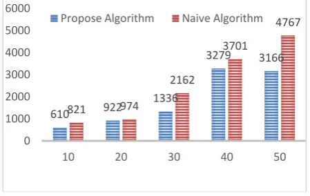
[image:3.595.315.540.539.681.2]

The Figure-2 shows a comparison between the traditional backtracking algorithms and propose algorithm. This comparison is done by taking variable size input vector and fixed capacity. The result shows that the propose algorithm batter than traditional backtracking algorithm. Here “x-axis” represents size of input vector and “y-axis” represents number of lines executed. The input elements for this experiment are describe in appendix-2 from input-2 to input-6.

Fig 2: Comparison between naive and Propose Algorithm by different input size vector and same capacity

0 1000 2000 3000 4000 5000 6000

1 5 9 13 17 21 25 29 33 37 41 45 49 53 57 Propose Algorithm Naive Algorithm

610 922

1336

3279 ₃₁₆₆

821 974

2162

3701

4767

0 1000 2000 3000 4000 5000 6000

10 20 30 40 50

(4)

23

4. CONCLUSION AND FUTURE WORK

The proposed algorithm ‘sum of subset’ problem provides all solutions of a given set of input vector and certain capacity. Simulation shows that the algorithm takes less number of steps as compared to traditional Naive algorithm. In future Time complexity of this algorithm can be analyze.

Apendix-1: Example

/* Level = Recurrence */

Step-1: Level-1

Search Set-A Total Set-B N.E N.S 30

Step-2: Level-1

Search Set-A Total Set-B

N.E N.S

30 {2,4,5,7,11} 29

Step-3: Level-1

N.E N.S

30 {2,4,5,7,11} 29

Remain-Set R'

{ 13 ,17 ,21 ,25 } {13 ,17 ,21 ,25 , (13,17) }

Step-4

/* ‘T’ ≠ ‘SE’, So this step skip */

Step-5 Level-1

N.E N.S

30 {2,4,5,7,11} 29 13

Remain-Set R'

{ 13 ,17 ,21 ,25 } {13 ,17 ,21 ,25 , (13,17) }

Step-6 Level-1

N.E N.S

30 {2,4,5,7,11} 29 13 13 12

Remain-Set R'

{ 13 ,17 ,21 ,25 } {13 ,17 ,21 ,25 , (13,17) }

/* Recurrence call again */

Step-1: Level-2

Step-2: Level-2

Search Set-A Total Set-B N.E N.S

12 {2,4,5} 11

Step-3: Level-2

Search Set-A Total Set-B N.E N.S 12 {2,4,5} 11

Remain-Set R' { 7,11 } {7, 11 }

Step-4

/* ‘T’ ≠ ‘SE’, So this step skip */

Step-5 Level-2

Search Set-A Total Set-B N.E N.S 12 {2,4,5} 11 7

Remain-Set R' { 7, 11 } {7, 11 }

Step-6 Level-2

Search Set-A Total Set-B N.E N.S

12 {2,4,5} 11 7 7 6

Remain-Set R' { 7, 11 } { 7, 11 }

/* Recurrence call again */

Step-1: Level-3

Step-2: Level-3

Search Set-A Total Set-B N.E N.S 6 {2,4} 6

Step-3: Level-3

Search Set-A Total Set-B N.E N.S 12 {2,4,5} 11

Remain-Set R'

{ 5 } { 5 }

Step-4 Level-3 ‘T’ == ‘SE’ Set flag=1; goto step-7;

Step-7 Level-3

FINAL MATRIX

Level Set-A Set-B

1 { 2, 4, 5, 7, 11 } {13}

2 { 2, 4, 5 } {7}

3 { 2, 4 } { }

Step-8

(5)

24 Return step-5

/* This process continue according to algorithm until get all solution */

Apendix-2: Describe Input vector ‘S’ for

Experiment

Input-1

S4={2,4,11,14,18,20,24,29,32,35,38,41,45,47,49,

51,56,57,63,66,69,73,77,79,82,84,91,95,97,99,

100,102,104,110,118,122,134,140,150,152,158,160,164 ,166,170,180,190,192,194,200}

Input-2

S5

=

{1,2,3,4,5,6,7,8,9,10}

Input-3

S6={2,11,20,23,28,29,32,33,35,38,40,41,45,48,49,51,56

,57,63,66} Input-4

S7={1,3,10,17,25,27,28,31,33,34,35,38,42,44,45,46,47,

49,51,55,56,57,61,67,68,69,74,79,82,89} Input-5

S8={1,2,4,9,14,20,30,31,35,37,38,40,42,44,47,48,

50,52,55,56,57,58,59,60,62,65,68,70,72,79,81,88, 89,91,92,93,94,97,99,100}

Input-6

S9={1,2,3,11,19,22,27,29,32,33,34,35,38,42,43,45,47,4

9,51,54,56,57,60,67,68,69,73,79,88,89,91,95,97,99,101, 102,104,110,119,122,133,140,150,152,

158,160,164,166,172,185}

Apendix-3: Simulation

The Simulation is Base on C programming Language, The outcome of our experiment shown below:

*/

Solution:

8. REFERENCES

[1] Yuli Ye, “Priority Algorithms for the Subset- Sum Problem” Master of Science Thesis, Graduate

Department of Computer Science University of Toronto”2006”.

[2] M. Garey and D. Johnson.Computers and Intractability : a Guide to the Theory of NP completeness. Freeman, 1979.

[3] L. Escudero, S. Martello, and P. Toth. A framework for tightening 0 - 1 programs based on extensions of pure 0-1 KP and SS problems.Lecture Notes in Computer Science, 920:110–123, 1995.

(6)

25 [5] O. Ibarra and C. Kim. Fast approximation algorithms

for the knapsack and sum of subset problem. Journal of the ACM, 22:463– 468, 1975.

[6] H. Kellerer, R. Mansini, U. Pferschy, and M. Speranza. An eﬃcient fully polynomial approximation scheme for the subset-sum problem. Journal of Computer and System Sciences, 66:349– 370, 2003.

[7] H. Kellerer , U. Pferschy, and D. Pisinger. Knapsack Problems. Springer, 2004.

[8] D. Pisinger. An exact algorithm for large multiple knapsack problems. European Journal of Operational Research, 114 : 528–541, 1999.

[9] A. Caprara and U. Pferschy. Packing bins with minima l slack. Technical report, University of Graz, 2002.

[10] B. Dietrich and L. Escudero. Coefficient reduction for knapsack constraints in 0-1 programs with VUBs. Operations Research Letters, 9:9–14, 1990.

[11] J. Hoogeveen, H. Oosterhout, and S. van de Velde. New lower and upper bounds for scheduling around a small common due date. Operations Research, 42 : 102–110-1994.