A Genetic Algorithm for the Split Delivery Vehicle Routing Problem

A Genetic Algorithm for the Split Delivery

Vehicle Routing Problem

Joseph Hubert Wilck IV1, Tom M. Cavalier2

1

Industrial and Information Engineering Department, University of Tennessee, Knoxville, USA

2

Industrial and Manufacturing Engineering Department, Pennsylvania State University, University Park, USA

Email: [email protected], [email protected]

Received February 18, 2012; revised March 20, 2012; accepted April 5, 2012

ABSTRACT

The Split Delivery Vehicle Routing Problem (SDVRP) allows customers to be assigned to multiple routes. Two hybrid genetic algorithms are developed for the SDVRP and computational results are given for thirty-two data sets from pre-vious literature. With respect to the total travel distance and computer time, the genetic algorithm compares favorably versus a column generation method and a two-phase method.

Keywords: Vehicle Routing Problem; Transportation; Genetic Algorithm

1. Introduction

The basic model for this paper is a vehicle routing prob- lem (VRP) variant, the split delivery vehicle routing problem (SDVRP). Standard forms of the VRP have been studied for decades as shown in the seminal paper by Dantzig and Ramser [1] and an algorithm developed by Clarke and Wright [2]. Recent surveys by Toth and Vigo [3] and Cordeau et al. [4,5] examine exact and heuristic procedures of the VRP, respectively. Golden and Assad [6] and Toth and Vigo [7] edited books solely devoted to the VRP and its variants, and Laporte and Osman [8] provide an extensive bibliography. Reimann [9] analyzed a vehicle routing problem with stochastic demands.

The SDVRP is appropriate for many CVRP applica- tions where customers can be visited more than once. Numerous applications for the CVRP are noted in the li- terature [6,7], with the primary emphasis being the dis- tribution of various goods. Dror and Trudeau [10,11] formally introduced the SDVRP. The primary motivation to split a customer’s demand over multiple routes is to reduce the travel distance and the number of vehicle routes. If each vehicle has the same capacity, then the minimum number of routes is the total demand divided by the vehicle capacity rounded up to the nearest integer.

Genetic algorithms have been used in a variety of areas [12]. There applications have been noted in many industrial engineering areas, including scheduling [13], vehicle routing [14], and the generalized orienteering problem [15].

2. Literature Review

2.1. Split Delivery Vehicle Routing Problem Literature Review

Dror and Trudeau [10,11] formally introduced the SD- VRP. The primary motivation to split a customer’s de- mand over multiple routes is to reduce the travel distance and the number of vehicle routes. If each vehicle has the same capacity, then the minimum number of routes is the total demand divided by the vehicle capacity rounded up to the nearest integer. They proved, given that the dis- tance between nodes follows the triangle inequality, there exists an optimal solution where no two routes can have more than one split demand point in common, and that there exists an optimal solution with no k-split cycles (for any k). Based on these proofs, Dror and Trudeau [11] devised a heuristic to solve the SDVRP given an initial CVRP solution by splitting a node’s demand to fill the routes to capacity. Dror et al. [16] extended the formu- lation of Dror and Trudeau [10,11] with additional con- straints, and developed a constraint relaxation branch and bound algorithm. The results from Dror and Trudeau [10, 11] and Dror et al. [16] show that the percent reduction in travel distance, when compared to the CVRP, is most prominent among problems where customers have high demands (i.e., more than 10% of the vehicle capacity). The results showed that the SDVRP solution used fewer routes than the CVRP solution; however, the SDVRP solution did not always use the minimum number of routes.

time windows on grid networks and developed heuristics to generate solutions. Archetti et al. [19] and Aleman and Hill [20] developed tabu search procedures for the SDVRP. Archetti et al. [21] analyzed the worst-case pro- perties of the SDVRP. Archetti et al. [22] discussed when demand splitting is most beneficial. Lee et al. [23] developed a dynamic programming model for the vehicle routing problem with split pick-ups with an uncountable (infinite) number of state and action spaces. Belenguer et al. [24] performed a polyhedral study on the SDVRP to produce lower bounds through formulating the problem with undirected arcs by assuming symmetric distances. Using a cutting-plane algorithm in conjunction with a relaxed formulation, they were able to obtain feasibility gaps within 12% for problems with 50, 75, and 100 customers. Jin et al. [25] developed a two-stage algo- rithm to solve the SDVRP using valid inequalities. Jin et al. [26,27] presented a column generation procedure that provides comparable lower and upper bounds for the data sets developed by Belenguer et al. [24]. Chen et al. [28] presented a mixed integer program and a variable length record-to-record travel algorithm. Burrows [29] showed that the SDVRP could be modified by splitting customer demand into smaller quantities on the same node, and then solved using CVRP methods. Wilck and Cavalier [30] developed a construction heuristic to quickly gene- rate feasible solutions to the SDVRP. Aleman et al. [31] present an adaptive memory algorithm for the SDVRP. Archetti and Speranza [32] and Gulczynski et al. [33] recently surveyed the SDVRP literature. Recent theses addressing the SDVRP include Aleman [34], Wilck [35], Liu [36], Nowak [37], and Chen [38].

Direct applications of the SDVRP have been noted in literature. Mullaseril et al. [39] modeled a cattle feed distribution problem as an SDVRP with time windows. Sierksma and Tijssen [40] model a helicopter crew- scheduling problem using an SDVRP model, developed a relaxed linear program and column generation scheme to find a solution, and used a cluster-and-route procedure. Song et al. [41] modeled a newspaper distribution proc- ess as a SDVRP and solved using a two-phase pro- cedure. The first phase allocates customers using a binary program and the second phase generates vehicle routes.

2.2. Genetic Algorithms in Vehicle Routing Problems Literature Review

A genetic algorithm is a global search procedure that solves problems by emulating evolution. A pure genetic algorithm uses reproduction and mutation to develop a new generation of solutions from the current generation of solutions. The constraints of the VRP do not allow the application of pure genetic algorithms without an addi- tional step to ensure feasibility.

The book by Goldberg [42] describes the solution

process of genetic algorithms. The Fundamental Theo- rem of Genetic Algorithms states the conditions in order to achieve a global optimal solution [43]. These condi- tions describe the breeding process and insist that better solutions (or patterns) remain in future generations while weaker solutions (or patterns) are eliminated from future generations. The typical genetic algorithm follows these basic steps [43].

The procedure outlined here is a basic genetic algori- thm. Procedures for generating feasible offspring and feasibly mutating the new generation are problem-spe- cific. For example, given a problem that can be repre- sented by a binary string with four values. Then the fol- lowing example can occur: Parent 1: 0-1-1-0 and Parent 2: 1-0-1-1.

A crossover will occur between any of the four values (i.e., between the first and second, between the second and third, and between the third and fourth). Based on probability (e.g., generating a random number between 0 and 1), the crossover point is chosen as between the second value and the third value. Thus the crossover will take 0-1 from Parent 1 and switch it with 1-0 from Parent 2, resulting in two offspring: Child 1: 1-0-1-0 and Child 2: 0-1-1-1. The mutation stage will then, using probability, randomly select a small number of offspring (if any at all) and change a small portion of position values. For example, suppose that based on probability, Child 2 is to be mutated in the second position. Originally, Child 2 is 0-1-1-1; and with muta- tion she is 0-0-1-1.

The preceding example assumed a binary string pro- blem structure with no limiting constraints. Unfortuna- tely, applying genetic algorithms directly to VRP va- riants is difficult due to the constraints of the problems. Therefore, additional steps or changes are necessary to ensure feasibility of created solutions. For VRP variants the reproduction stage (i.e., Step 4) can be modified to ensure feasible solutions or an additional step can be added after the mutation stage (i.e., Step 5) to fix in- feasible solutions.

straints of the VRP makes a genetic algorithm compu- tationally expensive.

Alvarenga et al. [14] developed a two-phase approach for the VRP with time windows by using a hybrid ge- netic algorithm and a set-partitioning method to generate routes. The two-phase approach yielded good solutions when compared to best known solutions. Solution time was not compared or reported, but the genetic algorithm was given a time limit of 60 minutes.

Baker and Ayechew [46] developed a pure genetic algorithm and a hybrid genetic algorithm for the CVRP while constraining the maximum distance of a route. The pure genetic algorithm produced poor solutions, when compared to previous simulated annealing and tabu search methods. The hybrid genetic algorithm provided comparable, although not superior, solutions when com- pared to previous methods in a reasonable amount of computer time. The hybrid genetic algorithm applied neighborhood search procedures to ensure a feasible so- lution.

Wang et al. [15] developed a genetic algorithm for the generalized orienteering problem. The orienteering pro- blem is a VRP variant where a start point and an end point are specified and other points have associated scores. The objective is to determine a path that maxi- mizes the score while adhering to a time constraint. The generalized orienteering problem (GOP) adds a level of complexity where there are numerous attributes at a specific point that represent the total score. The GOP is similar to a VRP with one vehicle route. The genetic algorithm developed by Wang et al. [15] compared favorably to an artificial neural network solution proce- dure. The genetic algorithm procedure initially allowed infeasible solutions, but then corrected the solutions by truncating them to accommodate the time constraint.

Jeon et al. [47] consider the VRP with multiple depots and up to two deliveries per node (i.e., split delivery). They developed a pure genetic algorithm and a hybrid genetic algorithm. The hybrid genetic algorithm ensured that no infeasible solutions were generated, and the hy- brid genetic algorithm provided consistently better re- sults in terms of objective value. Computation time was not provided for the pure genetic algorithm.

2.3. Data Sets from Previous Literature

Data sets from Belenguer et al. [24] and Chen et al. [28] were used to test the hybrid genetic algorithm procedure presented in this paper. The procedure was coded in FORTRAN 95 and compiled by GNU FORTRAN on an Intel Xeon Processor 2.49 GHz computer with 8 GB RAM. The number of customers and vehicles for 11 data sets from Belenguer et al. [24] are shown in Table 1. The number of customers ranged from 50 to 100, with an additional node for the depot. The data sets also differ by

Table 1. Eleven data sets from Belenguer et al. [24].

Data Set Customers Vehicles

S51D2 50 9

S51D3 50 15

S51D4 50 27

S51D5 50 23

S51D6 50 41

S76D2 75 15

S76D3 75 23

S76D4 75 37

S101D2 100 20

S101D3 100 31

S101D5 100 48

amount of spare capacity per vehicle. The customers were placed randomly around a central depot and de- mand was generated randomly based on a high and low threshold. The number of customers and vehicles for 21 data sets from Chen et al. [28] are shown in Table 2. The number of customers ranged from eight to 288, with an additional node for the depot. The data sets do not have any spare vehicle capacity. The customers were placed on rings surrounding a central depot and the demand was either 60 or 90, with a vehicle capacity of 100. Results from Jin et al. [26] and Chen et al. [28] were used as a comparison to the results from the hybrid genetic algo- rithm presented in this paper for these 32 data sets.

3. Hybrid Genetic Algorithm Procedure

A genetic algorithm is a global search procedure that solves problems by emulating evolution. A pure genetic algorithm uses reproduction and mutation to develop a new generation of solutions from the current generation of solutions. The constraints of the SDVRP do not allow the application of pure genetic algorithms without an additional step to ensure feasibility. A hybrid genetic algorithm allows for a genetic global search procedure while ensuring feasibility. The phrase hybrid genetic algorithm is sometimes used to describe memetic algo- rithms; however, for this paper hybrid refers to com- posing a solution from multiple sources. Coupling hybrid and genetic algorithms yields the term hybrid genetic algorithm. This section is organized as follows, Section 3.1 describes the development of an initial population and the reproduction procedure is discussed in Section 3.2.

3.1. Initial Population

Table 2. Twenty-one data sets from Chen et al. [28].

Data Set Customers Vehicles

S1 8 6

S2 16 12

S3 16 12

S4 24 18

S5 32 24

S6 32 24

S7 40 30

S8 48 36

S9 48 36

S10 64 48

S11 80 60

S12 80 60

S13 96 72

S14 120 90

S15 144 108

S16 144 108

S17 160 120

S18 160 120

S19 192 144

S20 240 180

S21 288 216

each of three controls. If the same set of rules is applied for three controls for each vehicle route, then up to 72 different solutions can be created. However, a more diverse set of solutions can be created if a different set of rules for each control is applied for each specific vehicle route within a solution. By randomly selecting which rule to apply for each specific control for each vehicle route, a feasible solution can be generated. Using this approach, 100 solutions with a random application of the rules were generated. These solutions were generated rather quickly, in less than 205 seconds for any particular data set. In order to provide the hybrid genetic algorithm with a strong and diverse start, the initial population for the hy- brid genetic algorithm included the 72 combination solu- tions (directly from the construction heuristic) and the 100 solutions generated by randomly applying the rules for each vehicle route.

3.2. Reproduction Procedures

The 100 randomly generated solutions and the 72 solu- tions developed by the construction heuristic were used as the initial population. Subsequent offspring popula- tions were created route-by-route using a hybrid genetic algorithm to ensure feasibility. A variety of parameter settings were analyzed and tuned based on the 32 data

sets. The results from two fitness approaches are given, shortest route and largest demand unit per distance unit.

3.2.1. Fitness Approach 1: Shortest Route

In order to build a single feasible solution a number of steps must be completed. The current population of so- lutions provides a set of vehicle routes, and these routes are sorted from shortest to longest based on travel dis- tance. The first fitness approach is to select shorter routes that meet a certain capacity threshold with a greater pro- bability of being selected than longer routes. The shortest feasible route is selected with a probability Pg, and this probability is the same for all solutions and routes. If the vehicle route is selected, then it is added to the current solution and is not included in any further solutions (neither the current solution nor any future solutions) for the current population. If the route is not selected, then the next shortest feasible route is selected with pro- bability Pg. If there are no feasible routes remaining, then the solution is completed using the construction heuristic with a random rule selection for the remaining vehicle routes. By using the construction heuristic, feasibility is ensured. In addition, a number of good solutions from the previous generation are included in the current gene- ration, and bad solutions generated were discarded. This is often referred to as memory [48,49]. This procedure ensures that each generation is better than the previous, and builds a set of good solutions.

The parameters are capacity threshold, probability of route being selected Pg, and the number of solutions from the previous generation kept in the current generation. These parameters were tuned using the 32 data sets. The results of this analysis were to set the capacity threshold as the average vehicle slack (rounded up). The proba- bility, Pg, of a route being selected was set to 20%. The number of solutions kept from the previous generation was set at 10%, which means that the worst 10% of the next generation solutions were discarded (unless they were more favorable than the best 10% from the previous generation). The population size for a generation was set at 100 solutions (except for the initial population which was 172 solutions) and the number of new generations is 20. These values were used to ensure the entire proce- dure was completed in a timely fashion.

taining feasibility.

The final solution outputted by the hybrid genetic algorithm is the best solution from the last generation. However, it is possible to find this solution in a previous generation, but it would have remained in the current generation since it would have been better than the worst 10% of solutions. This concept goes along with the sur- vival of the fittest goal of genetic algorithms.

3.2.2. Fitness Approach 2: Ratio of Demand Unit Versus Distance Unit

The first fitness approach uses only distances and does not take demand into account during the selection of routes. The second fitness approach sorts the feasible routes based on demand units divided by distance units. The larger this ratio, the more likely the route is selected. The route with the largest demand unit per distance unit is selected with probability Pg. All other parameters re- mained the same as Fitness Approach 1.

3.2.3. Step-by-Step Procedure for Hybrid Genetic Algorithm

Step 0: Build the initial population using the construc- tion heuristic and 100 random solutions by randomly applying the rules for each of the three controls. The total initial population size is 172.

Step 1: Build the current generation. Sort the routes in the previous population based on the fitness approach. Build a new solution iteratively by route by using Step 2.

Step 2: Select a feasible route with the best fitness value with probability Pg = 0.20. If the feasible route is selected, then add it to the current solution and discard it from being used in later solutions in the current genera-tion. If the feasible route is not selected, then repeat Step 2 (the feasible route is not discarded, but it is not allowed to be selected during the current iteration when selecting a vehicle route).

Step 3: Repeat Step 2 until a complete solution is built or until all feasible routes have been exhausted. If all feasible routes have been exhausted, then use the con- struction heuristic (by randomly applying the set of rules for each control) to build the remaining routes for the solution.

Step 4: Repeat Steps 2 and 3 until the entire population of 100 solutions is built.

Step 5: Compare the worst 10% of the current popula- tion of solutions to the best solutions from the previous generation. Select the best solutions (in terms of shortest travel distance) to remain in the current generation. At most 10 solutions from the current generation will be replaced.

Step 6: Repeat Step 1 until 20 generations are com- pleted.

Step 7: Select the best solution from the final genera-

tion. Output as final solution.

4. Computational Experience of the Hybrid

Genetic Algorithm

The hybrid genetic algorithm was applied to the data sets from Belenguer et al. [24] and Chen et al. [28] based on the Hybrid Genetic Algorithm Procedures described in Section 3 for both fitness approaches. The procedure was coded in FORTRAN 95 and compiled by GNU FORT- RAN on an Intel Xeon Processor 2.49 GHz computer with 8 GB RAM. The best solution was outputted as the final solution.

Section 4.1 describes the performance of the first fit- ness approach, with the 100 randomly generated solu- tions and the 72 solutions developed by the construction heuristic as the initial population. Section 4.2 describes performance, with the 100 randomly generated solutions and the 72 solutions developed by the construction heuri- stic as the initial population, using the second fitness approach.

4.1. Computational Experience Fitness Approach One

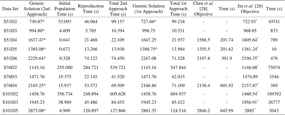
Comparative results for 11 data sets from Belenguer et al. [24] are shown in Table 3. The fitness approach one hybrid genetic algorithm time is separated into initial po- pulation time and reproduction time, and a total algori- thm time is provided. The genetic algorithm produced a solution in the least amount of computer time for each data set (bold), except S51D5. The hybrid genetic algo- rithm produced the solution with the least amount of travel distance in four cases (bold). Jin et al. [26] found a better solution for three data sets (bold) and Chen et al. [28] in four cases (bold). However, Jin et al. [26] allowed for additional vehicles in their solution, above the mini- mum number required for the SDVRP, which increases the cost of the overall system.

Table 3. Comparing the hybrid genetic algorithm (good start) versus the two-phase method of Chen et al. [28] and the column generation method of Jin et al. [26] for 11 data sets for the first fitness approach.

Data Set Genetic Solution

Initial Population

Time (s)

Reproduction Time (s)

Total Genetic Algorithm Time

(s)

Chen et al.

[28] Objective Time (s)

Jin et al. [26]

Objective Time (s)

S51D2 727.66^ 53.093 46.125 99.218 - - 722.93* 10741

S51D3 998.75 4.609 5.922 10.531 - - 968.85 833

S51D4 1647.25 0.641 21.296 21.937 1586.5 201.74 1605.64* ₇₈₉

S51D5 1388.75^ 0.672 13.312 13.984 1355.5 201.62 1361.24* ₁₀

S51D6 2267.08 0.328 71.000 71.328 2197.8 301.9 2196.35*

478

S76D2 1143.16 255.000 292.844 547.844 - - 1146.68* ₇₅₀₇₄

S76D3 1471.76 19.375 22.640 42.015 - - 1474.89 3546

S76D4 2166.86 15.937 55.172 71.109 2136.4 601.92 2157.87* ₃₆₉

S101D2 1458.76 356.734 248.203 604.937 - - 1460.54* ₁₈₉₃₉₂

S101D3 1945.23 38.969 46.453 85.422 - - 1956.91* ₃₆₇₇₇

S101D5 2881.35 6.969 117.547 124.516 2846.2 645.99 2885* 5043

*

Jin et al. [26] starred-solutions used more than the minimum number of vehicles, computer specifications unavailable, and computer solution time includes time to compute both lower and upper bounds; Chen et al. [28] cpu specifications: Visual Studio C++, CPLEX 9.0, Intel Pentium 4, 1.7 GHz, 512 MB RAM; Genetic Algorithm cpu specifications: FORTRAN 95, GNU, Intel Xeon, 2.49 GHz, 8 GB RAM; ^Genetic Algorithm improves upon the Initial Population from the Construction Heuristic and 100 Random Solutions.

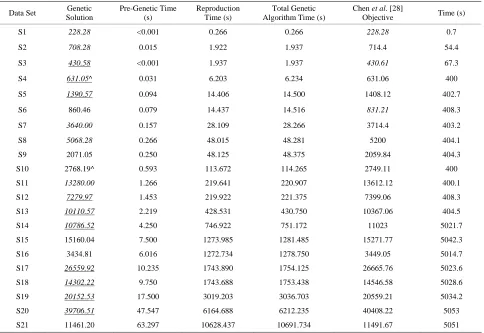
Table 4. Comparing the results of the hybrid genetic algorithm (good start) versus the two-phase method of Chen et al. [28] for 21 data sets for the first fitness approach.

Data Set Genetic Solution

Pre-Genetic Time (s)

Reproduction Time (s)

Total Genetic Algorithm Time (s)

Chen et al. [28]

Objective Time (s)

S1 228.28 <0.001 0.266 0.266 228.28 0.7

S2 708.28 0.015 1.922 1.937 714.4 54.4

S3 430.58 <0.001 1.937 1.937 430.61 67.3

S4 631.05^ 0.031 6.203 6.234 631.06 400

S5 1390.57 0.094 14.406 14.500 1408.12 402.7

S6 860.46 0.079 14.437 14.516 831.21 408.3

S7 3640.00 0.157 28.109 28.266 3714.4 403.2

S8 5068.28 0.266 48.015 48.281 5200 404.1

S9 2071.05 0.250 48.125 48.375 2059.84 404.3

S10 2768.19^ 0.593 113.672 114.265 2749.11 400

S11 13280.00 1.266 219.641 220.907 13612.12 400.1

S12 7279.97 1.453 219.922 221.375 7399.06 408.3

S13 10110.57 2.219 428.531 430.750 10367.06 404.5

S14 10786.52 4.250 746.922 751.172 11023 5021.7

S15 15160.04 7.500 1273.985 1281.485 15271.77 5042.3

S16 3434.81 6.016 1272.734 1278.750 3449.05 5014.7

S17 26559.92 10.235 1743.890 1754.125 26665.76 5023.6

S18 14302.22 9.750 1743.688 1753.438 14546.58 5028.6

S19 20152.53 17.500 3019.203 3036.703 20559.21 5034.2

S20 39706.51 47.547 6164.688 6212.235 40408.22 5053

S21 11461.20 63.297 10628.437 10691.734 11491.67 5051

underline).

4.2. Computational Experience Fitness Approach Two

Comparative results for 11 data sets from Belenguer et al. [24] are shown in Table 5. The second fitness approach hybrid genetic algorithm time is separated into initial population time and reproduction time, and a total gene- tic algorithm time is provided. Both fitness approaches produced the solution with the least amount of travel distance in four cases (bold). Jin et al. [26] found a better solution for three data sets (bold) and Chen et al. [28] in four cases (bold). However, Jin et al. [26] allowed for additional vehicles in their solution, above the minimum number required for the SDVRP, which increases the cost of the overall system.

Comparative results for 21 data sets from Chen et al. [28] are shown in Table 6. The second fitness approach found the solution with the least amount of travel dis- tance in 19 cases (bold). Chen et al. [28] found a better feasible solution for one data set (bold) (i.e., S6). Both methods found a solution with the same objective for data set S1. Chen et al. [28] reported pseudo lower bounds based on a graphical estimation described in Chen [38]. Chen et al. [28] finds a feasible solution that matches this pseudo lower bound for four instances (italic). The hybrid genetic algorithm (both fitness app- roaches) finds a feasible solution that matches this pseudo lower bound for five data sets (italic), and finds a feasible solution lower than this bound for ten data sets (italic and underline).

4.3. Fitness Approach Comparison

The second fitness approach found a better solution, when compared to the first approach, in six of the 11 data sets from Belenguer et al. [24], they tied in four cases (S76D2, S76D3, S101D2, S101D3), and the first app- roach found a better solution in only one data set (S51D2). In the four cases in which they tied, these were the four data sets in which the hybrid genetic algorithm outperformed Jin et al. [26] and Chen et al. [28]. For the 21 data sets from Chen et al. [28], when comparing the two fitness approaches, neither is consistently faster than the other in reproduction time. However, the second fitness approach finds a better solution in three cases (S6, S9, S10).

Based on the comparison between the two fitness app- roaches (with good initial solutions), neither approach seems to be faster than the other. Based on the 32 data sets the two methods were always within 5% of each other in reproduction runtime. However, the second fit- ness approach provides a better improvement in most cases, with the only exception being S51D2. The two approaches tie in many cases.

5. Summary

This paper focused on solving the SDVRP using a hybrid genetic algorithm. The primary research result of this paper are two fitness approaches for a hybrid genetic algorithm procedure that provide comparable solutions based on objective value and computer time for the SD- VRP when compared to a column generation procedure

Table 5. Comparing the hybrid genetic algorithm (second fitness approach) versus the two-phase method of Chen et al. [28] and the column generation method of Jin et al. [26] for 11 data sets.

Data Set

Genetic Solution (2nd

Approach)

Initial Population

Time (s)

Reproduction Time (s)

Total 2nd Approach Time (s)

Genetic Solution (1st Approach)

Total 1st Approach Time (s)

Chen et al. [28] Objective

Time (s) Jin et al. [26] Objective Time (s)

S51D2 730.87^ 53.093 46.064 99.157 727.66^ 99.218 - - 722.93* ₁₀₇₄₁

S51D3 994.80^ 4.609 5.785 10.394 998.75 10.531 - - 968.85 833

S51D4 1637.47^ 0.641 21.468 22.109 1647.25 21.937 1586.5 201.74 1605.64* ₇₈₉

S51D5 1385.08^ 0.672 13.266 13.938 1388.75^ 13.984 1355.5 201.62 1361.24* ₁₀

S51D6 2229.64^ 0.328 74.122 74.450 2267.08 71.328 2197.8 301.9 2196.35* ₄₇₈

S76D2 1143.16 255.000 284.721 539.721 1143.16 547.844 - - 1146.68* ₇₅₀₇₄

S76D3 1471.76 19.375 22.145 41.520 1471.76 42.015 - - 1474.89 3546

S76D4 2165.25^ 15.937 53.572 69.509 2166.86 71.109 2136.4 601.92 2157.87* ₃₆₉

S101D2 1458.76 356.734 248.894 605.628 1458.76 604.937 - - 1460.54* ₁₈₉₃₉₂

S101D3 1945.23 38.969 45.486 84.455 1945.23 85.422 - - 1956.91* ₃₆₇₇₇

S101D5 2873.08^ 6.969 120.897 127.866 2881.35 124.516 2846.2 645.99 2885* ₅₀₄₃

*_{Jin et al. [26] starred-solutions used more than the minimum number of vehicles, computer specifications unavailable, and computer solution time includes}

Table 6. Comparing the hybrid genetic algorithm (second fitness approach) versus the two-phase method of Chen et al. [28] for 21 data sets.

Data Set

Genetic Solution (Second

Approach)

Initial Population

Time (s)

Reproduction Time (s)

Total Second Approach Time (s)

Genetic Solution (First Approach)

Total First Approach Time (s)

Chen et al. [28] Objective Time (s)

S1 228.28 <0.001 0.272 0.272 228.28 0.266 228.28 0.7

S2 708.28 0.015 1.935 1.950 708.28 1.937 714.4 54.4

S3 430.58 <0.001 1.939 1.939 430.58 1.937 430.61 67.3

S4 631.05^ 0.031 6.207 6.238 631.05^ 6.234 631.06 400

S5 1390.57 0.094 14.104 14.198 1390.57 14.500 1408.12 402.7

S6 833.58^ 0.079 14.887 14.966 860.46 14.516 831.21 408.3

S7 3640.00 0.157 28.453 28.610 3640.00 28.266 3714.4 403.2

S8 5068.28 0.266 47.994 48.260 5068.28 48.281 5200 404.1

S9 2054.84^ 0.250 48.655 48.905 2071.05 48.375 2059.84 404.3

S10 2746.54^ 0.593 113.564 114.157 2768.19^ 114.265 2749.11 400

S11 13280.00 1.266 230.377 231.643 13280.00 220.907 13612.12 400.1

S12 7279.97 1.453 225.656 227.109 7279.97 221.375 7399.06 408.3

S13 10110.57 2.219 419.732 421.951 10110.57 430.750 10367.06 404.5

S14 10786.52 4.250 714.396 718.646 10786.52 751.172 11023 5021.7

S15 15160.04 7.500 1270.850 1278.350 15160.04 1281.485 15271.77 5042.3

S16 3433.83^ 6.016 1219.865 1225.881 3434.81 1278.750 3449.05 5014.7

S17 26559.92 10.235 1711.962 1722.197 26559.92 1754.125 26665.76 5023.6

S18 14302.22 9.750 1726.084 1735.834 14302.22 1753.438 14546.58 5028.6

S19 20152.53 17.500 3075.671 3093.171 20152.53 3036.703 20559.21 5034.2

S20 39706.51 47.547 6160.615 6208.162 39706.51 6212.235 40408.22 5053

S21 11461.20 63.297 10502.406 10565.703 11461.20 10691.734 11491.67 5051

Chen et al. [28] cpu specifications: Visual Studio C++, CPLEX 9.0, Intel Pentium 4, 1.7 GHz, 512 MB RAM; Genetic Algorithm cpu specifications: FOR-TRAN 95, GNU, Intel Xeon, 2.49 GHz, 8 GB RAM; ^Genetic Algorithm improves upon the Initial Population from the Construction Heuristic and 100 Ran-dom Solutions.

[26] and a two-step method [28]. Of the two fitness approaches, the second fitness approach performed better for most of the 32 data sets in terms of solution quality. Neither fitness approach was better than the other in solution time. The hybrid genetic algorithm does not assume symmetric distances, and a future research dire- ction would be to test this heuristic with asymmetric data sets.

REFERENCES

[1] G. B. Dantzig and J. H. Ramser, “The Truck Dispatching Problem,” Management Science, Vol. 6, No. 1, 1959, pp. 80-91. doi:10.1287/mnsc.6.1.80

[2] G. Clarke and J. Wright, “Scheduling of Vehicles from a Central Depot to a Number of Delivery Points,” Opera-tions Research, Vol. 12, No. 4, 1964, pp. 568-581. doi:10.1287/opre.12.4.568

[3] P. Toth and D. Vigo, “Models, Relaxations and Exact Approaches for the Capacitated Vehicle Routing Prob-lem,” Discrete Applied Mathematics, Vol. 123, No. 1-3, 2002, pp. 487-512.

doi:10.1016/S0166-218X(01)00351-1

[4] J. F. Cordeau, M. Gendreau, G. Laporte, J.-Y. Potvin and F. Semet, “A Guide to Vehicle Routing Heuristics,” Jour- nal of the Operational Research Society, Vol. 53, 2002, pp. 512-522. doi:10.1057/palgrave.jors.2601319

[5] J. F. Cordeau, M. Gendreau, A. Hertz, G. Laporte and J. S. Sormany, “New Heuristics for the Vehicle Routing Prob-lem,” In: A. Langevin and D. Riopel, Eds., Logistics Sys-tems: Design and Optimization, Springer, 2005, pp. 270- 297. doi:10.1007/0-387-24977-X_9

[6] B. L. Golden and A. A. Assad, “Vehicle Routing: Meth-ods and Studies,” North-Holland, Amsterdam, 1988.

[7] P. Toth and D. Vigo, “The Vehicle Routing Problem,” Society for Industrial and Applied Mathematics, Phila-delphia, 2002.

[8] G. Laporte and I. H. Osman, “Routing Problems: A Bib-liography,” Annals of Operations Research, Vol. 61, No. 1, 1995, pp. 227-262. doi:10.1007/BF02098290

[9] M. Reimann, “Analysing Risk Orientation in a Stochastic VRP,” European Journal of Industrial Engineering, Vol. 1, No. 2, 2007, pp. 111-130.

[10] M. Dror and P. Trudeau, “Savings by Split Delivery Routing,” Transportation Science, Vol. 23, No. 2, 1989, pp. 141-145. doi:10.1287/trsc.23.2.141

[11] M. Dror and P. Trudeau, “Split Delivery Routing,” Naval Research Logistics, Vol. 37, 1990, pp. 383-402.

[12] M. Affenzeller, S. Winkler, S. Wagner and A. Beham, “Genetic Algorithms and Genetic Programming: Modern Concepts and Practical Applications (Numerical Insights),” Chapman & Hall, 2009. doi:10.1201/9781420011326 [13] P. Damodaran, N. S. Hirani and M. C. Velez-Gallego,

“Scheduling Identical Parallel Batch Processing Machines to Minimise Makespan Using Genetic Algorithms,” Euro-pean Journal of Industrial Engineering, Vol. 3, No. 2, 2009, pp. 187-206. doi:10.1504/EJIE.2009.023605 [14] G. B. Alvarenga, G. R. Mateus and G. de Tomi, “A

Ge-netic and Set Partitioning Two-Phase Approach for the Vehicle Routing Problem with Time Windows,” Com-puters & Operations Research, Vol. 34, No. 6, 2007, pp. 1561-1584. doi:10.1016/j.cor.2005.07.025

[15] X. Wang, B. L. Golden and E. A. Wasil, “Using a Genetic Algorithm to Solve the Generalized Orienteering Prob-lem,” In: B. Golden, S. Raghavan and E. Wasil, Eds., The Vehicle Routing Problem: Latest Advances and New Chal-lenges, Springer, 2008, pp. 263-274.

doi:10.1007/978-0-387-77778-8_12

[16] M. Dror, G. Laporte and P. Trudeau, “Vehicle Routing with Split Deliveries,” Discrete Applied Mathematics, Vol. 50, No. 3, 1994, pp. 239-254.

doi:10.1016/0166-218X(92)00172-I

[17] P. W. Frizzell and J. W. Giffin, “The Split Delivery Ve-hicle Scheduling Problem With Time Windows and Grid Network Distances,” Computers and Operations Re-search, Vol. 22, No. 6, 1995, pp. 655-667.

doi:10.1016/0305-0548(94)00040-F

[18] P. W. Frizzell and J. W. Giffin, “The Bounded Split De-livery Vehicle Routing Problem with Grid Network Dis-tances,” Asia Pacific Journal of Operational Research, Vol. 9, 1992, pp. 101-116.

[19] C. Archetti, M. Savelsbergh and A. Hertz, “A Tabu Search Algorithm for the Split Delivery Vehicle Routing Problem,” Transportation Science, Vol. 40, No. 1, 2006, pp. 64-73. doi:10.1287/trsc.1040.0103

[20] R. E. Aleman and R. R. Hill, “A Tabu Search with Vo-cabulary Building Approach for the Vehicle Routing Problem with Split Demands,” International Journal of Metaheuristics, Vol. 1, No. 1, 2010, pp. 55-80.

[21] C. Archetti, M. Savelsbergh and M. G. Speranza, “Worst-Case Analysis for Split Delivery Vehicle Routing Problems,” Transportation Science, Vol. 40, No. 2, 2006, pp. 226-234. doi:10.1287/trsc.1050.0117

[22] C. Archetti, M. Savelsbergh and M. G. Speranza, “To Split or Not to Split: That Is the Question,” Transporta-tion Research Part E, Vol. 44, No. 1, 2008, pp. 114-123. doi:10.1016/j.tre.2006.04.003

[23] C. Lee, M. A. Epelman, C. C. White and Y. A. Bozer, “A Shortest Path Approach to the Multiple-Vehicle Routing Problem with Split Pick-Ups” Transportation Research Part B, Vol. 40, No. 4, 2006, pp. 265-284.

doi:10.1016/j.trb.2004.11.004

[24] J. M. Belenguer, M. C. Martinez and E. A. Mota, “Lower Bound for the Split Delivery VRP,” Operations Research, Vol. 48, No. 5, 2000, pp. 801-810.

doi:10.1287/opre.48.5.801.12407

[25] M. Jin, K. Liu and R. O. Bowden, “A Two-Stage Algo-rithm with Valid Inequalities for the Split Delivery Vehi-cle Routing Problem,” International Journal of Produc-tion Economics, Vol. 105, No. 1, 2007, pp. 228-242. doi:10.1016/j.ijpe.2006.04.014

[26] M. Jin, K. Liu and B. Eksioglu, “A Column Generation Algorithm for the Vehicle Routing Problem with Split Delivery,” Proceedings of the 2007 Industrial Engineer-ing Research Conference, Nashville, 19-23 May 2007.

[27] M. Jin, K. Liu and B. Eksioglu, “A Column Generation Approach for the Split Delivery Vehicle Routing Prob-lem,” Operations Research Letters, Vol. 36, No. 2, 2008, pp. 265-270. doi:10.1016/j.orl.2007.05.012

[28] S. Chen, B. Golden and E. Wasil, “The Split Delivery Vehicle Routing Problem: Applications, Test Problems, and Computational Results,” Networks, Vol. 49, No. 4, 2007, pp. 318-329. doi:10.1002/net.20181

[29] W. Burrows, “The Vehicle Routing Problem with Loads-plitting: A Heuristic Approach,” 24th Annual Conference of the Operational Research Society of New Zealand, Auckland, 18-19 August 1988, pp. 33-38.

[30] J. H. Wilck IV and T. M. Cavalier, “A Construction Heu-ristic for the Split Delivery Vehicle Routing Problem,”

American Journal of Operations Research, 2012, in press.

[31] R. E. Aleman, X. Zhang and R. R. Hill, “An Adaptive Memory Algorithm for the Split Delivery Routing Prob-lem,” Journal of Heuristics, 2008, Available Online.

[32] C. Archetti and M. G. Speranza, “The Split Delivery Ve-hicle Routing Problem: A Survey. The VeVe-hicle Routing Problem: Latest Advances and New Challenges,” Opera-tions Research/Computer Science Interfaces Series, Vol. 43, Part I, 2008, pp. 103-122.

doi:10.1007/978-0-387-77778-8_5

[33] D. J. Gulczynski, B. Golden and E. Wasil, “Recent De-velopments in Modeling and Solving the Split Delivery Vehicle Routing Problem,” Tutorials in Operations Re-search, INFORMS, 2008, pp. 170-180.

[34] R. E. Aleman, “A Guided Neighborhood Search Applied to the Split Delivery Vehicle Routing Problem,” Disserta-tion Thesis, Wright State University, 2009.

[35] J. H. Wilck IV, “Solving the Split Delivery Vehicle Rout-ing Problem,” Dissertation Thesis, Pennsylvania State University, 2009.

[36] K. Liu, “A Study on the Split Delivery Vehicle Routing Problem,” Dissertation Thesis, Mississippi State Univer-sity, 2005.

[37] M. A. Nowak, “The Pickup and Delivery Problem with Split Loads,” Dissertation Thesis, Georgia Institute of Technology, 2005.

2007.

[39] P. Mullaseril, M. Dror and J. Leung, “Split-Delivery Routing Heuristics in Livestock Feed Distribution,” Jour- nal of the Operational Research Society, Vol. 48, 1997, pp. 107-116.

[40] G. Sierksma and G. A. Tijssen, “Routing Helicopters for Crew Exchanges on Off-Shore Locations,” Annals of Operations Research, Vol. 76, 1998, pp. 261-286. doi:10.1023/A:1018900705946

[41] S. Song, K. Lee and G. Kim, “A Practical Approach to Solving a Newspaper Logistics Problem Using a Digital Map,” Computers and Industrial Engineering, Vol. 43, No. 1-2, 2002, pp. 315-330.

doi:10.1016/S0360-8352(02)00077-3

[42] D. Goldberg, “Genetic Algorithms in Search Optimiza-tion and Machine Learning,” Addison Wesley, Reading, 1989.

[43] W. L. Winston and M. Venkataramanan, “Introduction to Mathematical Programming, Operations Research: Vol-ume One,” 4th Edition, Thomson Learning, 2003.

[44] M. Gendreau, G. Laporte and J.-Y. Potvin, “Vehicle Routing: Modern Heuristics,” In: E. Aarts and J. K. Len-stra, Eds., Local Search in Combinatorial Optimization,

John Wiley & Sons, Inc., New York, 1997, pp. 323-330.

[45] M. Gendreau, G. Laporte and J.-Y. Potvin, “Metaheuris-tics for the Capacitated VRP,” In: P. Toth and D. Vigo, Eds., The Vehicle Routing Problem, Society for Industrial and Applied Mathematics, Philadelphia, 2002, pp. 140- 144.

[46] B. M. Baker and M. A. Ayechew, “A Genetic Algorithm for the Vehicle Routing Problem,” Computers & Opera-tions Research, Vol. 30, No. 5, 2003, pp. 787-800. doi:10.1016/S0305-0548(02)00051-5

[47] G. Jeon, H. R. Leep and J. Y. Shim, “A Vehicle Routing Problem Solved by Using a Hybrid Genetic Algorithm,”

Computers & Industrial Engineering, Vol. 53, No. 4, 2007, pp. 680-692. doi:10.1016/j.cie.2007.06.031

[48] S. J. Louis and G. Li, “Augmenting Genetic Algorithms with Memory to Solve Traveling Salesman Problems,”

Proceedings of the Joint Conference on Information Sci-ences, 1997.

[49] A. Acan and Y. Tekol, “Chromosome Reuse in Genetic Algorithms,” Lecture Notes in Computer Science, GECCO