Study on the Macro Level Risk Assessment and Intelligent Line Selection for Overseas Railway Construction

https://www.scirp.org/journal/ajibm ISSN Online: 2164-5175

ISSN Print: 2164-5167

DOI: 10.4236/ajibm.2019.911136 Nov. 29, 2019 2064 American Journal of Industrial and Business Management

Study on the Macro-Level Risk Assessment and

Intelligent Line Selection for Overseas Railway

Construction

Jing Lian

, Jing Jin

, Zonghao Li

1_{Department of Engineering Economics, Design Institute of China Railway Academy Co., Ltd, Chengdu, China} 2_{China Academy of Railway Sciences, Beijing, China}

3_{Department of Civil Engineering, Southwest Jiaotong University, Chengdu, China}

Abstract

In recent years, China has made overseas railway construction a key invest-ment project. The primary task of overseas railway investinvest-ment construction is to select railway routes. Taking some sections of the Belt and Road as an ex-ample, 15 representative risk indicators have been established based on the survey data. Based on the principal component analysis method, the risk as-sessment is carried out in 63 countries along the Belt and Road district, and finally the risk scores are sorted, and the reasonable high-speed rail lines are programmed through the ranking of risk scores.

Keywords

Railway Route Selection, Principal Component Analysis Method, Risk Assessment

1. Introduction

Since the establishment of “the Belt and Road” cooperation in 2013, China’s com-mitment to overseas railway investment and construction can not only drive the economic development of China and neighboring countries, but also demon-strate China’s economic strength and the development of high-speed rail tech-nology.

The primary task of the construction of overseas high-speed railway is railway route selection. The design of railway route selection is the overall design of a railway line, which directly affects the railway transportation capacity, transpor-tation quality and economic benefits of investment. Because the work load of How to cite this paper: Lian, J., Jin, J. and

Li, Z.H. (2019) Study on the Macro-Level Risk Assessment and Intelligent Line Selec-tion for Overseas Railway ConstrucSelec-tion. American Journal of Industrial and Busi-ness Management, 9, 2064-2077.

https://doi.org/10.4236/ajibm.2019.911136

Received: September 18, 2019 Accepted: November 26, 2019 Published: November 29, 2019

Copyright © 2019 by author(s) and Scientific Research Publishing Inc. This work is licensed under the Creative Commons Attribution International License (CC BY 4.0).

DOI: 10.4236/ajibm.2019.911136 2065 American Journal of Industrial and Business Management constructing a new railway (especially the oversea railways) is very large, and the technology is complex and widely involved. Therefore, before planning a rail-way, in-depth investigation and research, survey and design work must be car-ried out, and an optimal solution should be selected from several comparable solutions in the end. The Belt and Road Initiative involves many countries, and each country has different conditions. Therefore, it is necessary to use a unified standard to conduct risk assessments for all countries, and there are many me-thods for risk assessment. Choosing the appropriate method has a key role in risk assessment [1].

In this paper, the principal component analysis method is finally used for evalu-ation. The advantages are as follows:

1) The principal component analysis can eliminate the correlation between evaluation indicators Because the principal component analysis forms the prin-cipal components that are independent of each other after transforming the original index variables, and the higher the degree of correlation between the in-dicators is proved, the better the principal component analysis is.

2) The principal component analysis can reduce the workload of indicator se-lection for other evaluation methods; it is difficult to eliminate the correlation between the evaluation indicators, so it takes a lot of effort to select the indica-tors. While the principal component analysis can eliminate the related influ-ences, so it is relatively easy to select the indicators.

3) When there are more rating indicators, it is also possible to use a few com-prehensive indicators instead of the original indicators for analysis while retain-ing most of the information. In the principal component analysis, the principal components are arranged in order of variance. When analyzing the problem, some of the principal components can be discarded, and only the principal com-ponents with larger pre and post variance are used to represent the original va-riables, thus reducing the computational workload.

4) In the comprehensive evaluation function, the weight of each principal com-ponent is its contribution rate, which reflects the proportion of the information of the primary component of the original data to the total amount of informa-tion, so that the determination of the weight is objective and reasonable, and it overcomes the defect of artificially determining the weight in some evaluation methods.

5) The calculation of this method is relatively standardized, which can be eas-ily implemented on a computer, and can be done with specialized software.

2. Macro-Level Risk Indicators

in-DOI: 10.4236/ajibm.2019.911136 2066 American Journal of Industrial and Business Management dicators are selected here, namely, political, economic, and social development- related specific factors to reflect the specific situation of each country [2].

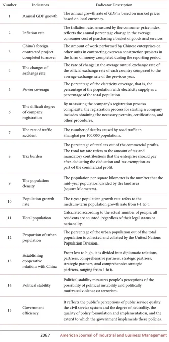
In consultation with Dr. Tong Xinhao, Dr. Zeng Hailin and other experts (both professors in the railway industry from Southwest Jiaotong University) and based on the actual situation of countries along the railway, the macro-level risk as-sessment indicators are comprehensively selected of data from various authorita-tive databases on railway line selection and data on foreign project contracting and import and export in China, which are shown in Table 1.

3. Macro-Level Risk Assessment and Route Selection

3.1. Macro-Level Risk Assessment Principle [3] [4]

Principal component analysis is a multivariate statistical technique that trans-forms a set of possible correlation variables into a set of linearly uncorrelated va-riables by orthogonal transformation. The converted set of vava-riables is called the principal component. The basic idea is to reduce the dimensionality of the orig-inal variable data to obtain several principal component integrated variables that are not related to each other instead of a large number of original variables, and these integrated variables carry most of the information in the original variables [3]. The first comprehensive variable selected is denoted as F1, and F1 has the largest Var(F1), which means that F1 contains the largest amount of information, and F1 is called the first principal component. If the first principal component is insufficient to represent the information carried by the original p variables, then the second principal component F2 is selected, and F2 is independent of F1 linear, and the mathematical language expression requires Cov(F1, F2) = 0. By analogy, the third principal component and the fourth principal component can be con-structed up to the No. p principal component.

This article uses related software to perform principal component analysis. The main steps are as follows:

1) Normalizing raw data.

In order to make the indicators comparable, the first thing is eliminating the different dimensions of each indicator and standardizing the indicators to obtain standardized data. This standardized process is actually doing the following trans-formation on the raw data X:

( )

(

)

ij j

ij

j

x x

ZX i n j p

Var x

−

= =  = 

in which:

( )

(

)

2

1 _, 1

1

n n

ij ij j

i i

j j

x x x

x Var x

n n

= =

−

= =

−

∑

∑

DOI: 10.4236/ajibm.2019.911136 2067 American Journal of Industrial and Business Management

Table 1. Macro-level risk assessment indicators for overseas railway construction.

Number Indicators Indicator Description

1 Annual GDP growth The annual growth rate of GDP is based on market prices _{based on local currency.}

2 Inflation rate The inflation rate, measured by the consumer price index, reflects the annual percentage change in the average consumer cost of purchasing a basket of goods and services.

3 China’s foreign contracted project completed turnover

The amount of work performed by Chinese enterprises or other units in contracting overseas construction projects in the form of money completed during the reporting period.

4 The changes of _{exchange rate} The rate of change in the average annual exchange rate of the official exchange rate of each country compared to the average exchange rate of the previous year.

5 Power coverage The percentage of the electricity coverage, that is, the percentage of the population with electricity supply as a percentage of the total population.

6 The difficult degree of company registration

By measuring the company’s registration process complexity, the registration process for starting a company includes obtaining the necessary permits, certifications, and other procedures.

7 The rate of traffic _accident The number of deaths caused by road traffic in _{Shanghai per 100,000 populations.}

8 Tax burden

The percentage of total tax out of the commercial profits. The total tax rate refers to the amount of tax and mandatory contributions that the enterprise should pay after deducting the deduction and tax exemption as part of the commercial profit.

9 The population _density The population per square kilometer is the number that the mid-year population divided by the land area (square kilometers).

10 Population growth _rate The t-year population growth rate refers to the _{medium-term population growth rate from t-1 to t.}

11 Total population Calculated according to the actual number of people, all residents are counted, regardless of their legal status or nationality.

12 Proportion of urban _population The percentage of the urban population out of the total population is collected and collated by the United Nations Population Division.

13 Establishing cooperative relations with China

From low to high, it is divided into diplomatic relations, partners, comprehensive partners, strategic partners, strategic partners, and comprehensive strategic partners, ranging from 1 to 6.

14 Political stability Political stability measures people’s perceptions of the possibility of political instability and politically motivated violence or terrorism.

15 Government _efficiency

DOI: 10.4236/ajibm.2019.911136 2068 American Journal of Industrial and Business Management 4) Calculating the variance contribution rate and the cumulative contribution rate of each principal component.

The contribution rate of the main component Fi:

(

)

1

1, 2, ,

i

i p

k k

i p

λ

α

λ

=

= =

∑

Cumulative contribution rate:

1

1

m

k k

p

k k

λ β

λ =

=

=

∑

∑

In the practical application of the principal component analysis method, the cor-responding first, second, …, m-th main components to the λ λ1, 2,,λm (m≤ p)

are chosen, in which the, λ λ1, 2,,λm (m≤ p) of the eigenvalues must be the

those that cumulative contribution rate is higher than 60%.

5) Calculating the principal component coefficients and principal component scores.

Let the load matrix be A, then the coefficient of the principal component Fi is the square root of each load matrix divided by the square root of the corres-ponding principal component variance, and propose the coefficient of Fi is the matrix Ci, then the score of the principal component Fi is:

i i i

Z =C ×ZX

where ZXi represents the i-th column of the matrix ZX of data normalization. 6) Comprehensive score assessment.

The first m principal components with cumulative contribution rate of 60% are selected, and take the variance contribution rate αk (k=1, 2,,m) as the

weight to construct a linear combination as a comprehensive evaluation func-tion:

1 1 2 2 m m

R=αZ +α Z + + α Z

From the above formula, the comprehensive score R of the evaluation can be obtained, and then the magnitude of the R value is calculated according to the value of each data of each evaluation object and these R values are comprehen-sively sorted, thereby obtaining a comprehensive evaluation of each object to be evaluated [5].

3.2. Instance Application

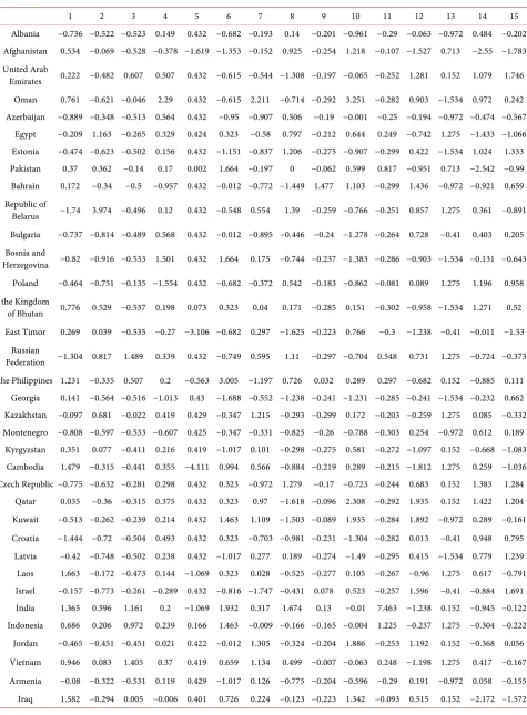
dif-DOI: 10.4236/ajibm.2019.911136 2069 American Journal of Industrial and Business Management ference between the dimensions Large, it is necessary to standardize the various risk data, and use the unified standard to judge, so the original data is first stan-dardized, and the standardized data is shown in Table 2[6].

The normalized data is used in the dimension reduction factor analysis, and the data is subjected to KMO and Bartley test. If the result of KMO value is greater than 0.6 and the significance of the Bartley test is less than 0.01, principal com-ponent analysis or factor analysis can be performed. Because the amount of samples are huge, so on the basis of principal component analysis, the rotation of the factors is actually rotating the factor load matrix, which can simplify the structure of the factor load matrix, so that the square of the element of each column or row in the load matrix is polarized to 0 and 1, through the factor ro-tation (actually coordinate roro-tation), it makes each original variable have a close relationship between as few factors as possible, so the actual meaning of the fac-tor solution is easier to explain [7].

Then, the factor analysis tool is used for dimensionality reduction. Based on the principal component analysis, the maximum variance method is used to perform the factor rotation, and the result Table 3 is obtained.

It can be seen from the above test results that the KMO value is greater than 0.6 and the significance is less than 0.01, so it is suitable for principal component analysis or factor analysis.

As can be seen from Table 4, the first five principal components contain nearly 66% of the information, and it can be considered that these five principal com-ponents contain most of the information of the original elements.

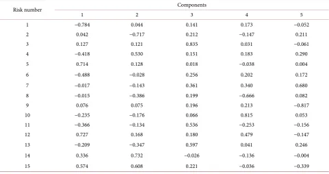
The load matrix after the rotation of these five principal components is shown in Table 5, the coefficient indicating the risk of each component, generally greater than 0.5 - 0.6, is attributed to the component.

The above data was processed to obtain Table 6, where the gray shading marks were the portions with coefficients greater than 0.58.

Name each principal component according to the data marked in the below table.

The fifth item (power coverage rate) and the 12th item of urbanization rate in F1 have large coefficients. These two indicators are related to the level of urban development. Therefore, F1 is called “the main component of urban moderniza-tion level”;

The 14th (political stability) and 15th (government efficiency) factors in F2 are relatively large. Both of these indicators are related to the political situation, so F2 is called “the main component of the political environment”;

The third item in F3 (the turnover of China’s foreign contracted projects) and the 13th (the establishment of cooperative relations with China) have a large coef-ficient. These two indicators are related to bilateral cooperation, so F3 is called “bilateral with China”. The main component of the partnership;

DOI: 10.4236/ajibm.2019.911136 2070 American Journal of Industrial and Business Management

Table 2. Standardized data.

1 2 3 4 5 6 7 8 9 10 11 12 13 14 15

Albania −0.736 −0.522 −0.523 0.149 0.432 −0.682 −0.193 0.14 −0.201 −0.961 −0.29 −0.063 −0.972 0.484 −0.202 Afghanistan 0.534 −0.069 −0.528 −0.378 −1.619 −1.353 −0.152 0.925 −0.254 1.218 −0.107 −1.527 0.713 −2.55 −1.783 United Arab

Emirates 0.222 −0.482 0.607 0.507 0.432 −0.615 −0.544 −1.308 −0.197 −0.065 −0.252 1.281 0.152 1.079 1.746 Oman 0.761 −0.621 −0.046 2.29 0.432 −0.615 2.211 −0.714 −0.292 3.251 −0.282 0.903 −1.534 0.972 0.242 Azerbaijan −0.889 −0.348 −0.513 0.564 0.432 −0.95 −0.907 0.506 −0.19 −0.001 −0.25 −0.194 −0.972 −0.474 −0.567

Egypt −0.209 1.163 −0.265 0.329 0.424 0.323 −0.58 0.797 −0.212 0.644 0.249 −0.742 1.275 −1.433 −1.066 Estonia −0.474 −0.623 −0.502 0.156 0.432 −1.151 −0.837 1.206 −0.275 −0.907 −0.299 0.422 −1.534 1.024 1.333 Pakistan 0.37 0.362 −0.14 0.17 0.002 1.664 −0.197 0 −0.062 0.599 0.817 −0.951 0.713 −2.542 −0.99 Bahrain 0.172 −0.34 −0.5 −0.957 0.432 −0.012 −0.772 −1.449 1.477 1.103 −0.299 1.436 −0.972 −0.921 0.659 Republic of

Belarus −1.74 3.974 −0.496 0.12 0.432 −0.548 0.554 1.39 −0.259 −0.766 −0.251 0.857 1.275 0.361 −0.891 Bulgaria −0.737 −0.814 −0.489 0.568 0.432 −0.012 −0.895 −0.446 −0.24 −1.278 −0.264 0.728 −0.41 0.403 0.205 Bosnia and

Herzegovina −0.82 −0.916 −0.533 1.501 0.432 1.664 0.175 −0.744 −0.237 −1.383 −0.286 −0.903 −1.534 −0.131 −0.643 Poland −0.464 −0.751 −0.135 −1.554 0.432 −0.682 −0.372 0.542 −0.183 −0.862 −0.081 0.089 1.275 1.196 0.958 the Kingdom

of Bhutan 0.776 0.529 −0.537 0.198 0.073 0.323 0.04 0.171 −0.285 0.151 −0.302 −0.958 −1.534 1.271 0.52 East Timor 0.269 0.039 −0.535 −0.27 −3.106 −0.682 0.297 −1.625 −0.223 0.766 −0.3 −1.238 −0.41 −0.011 −1.53

Russian

Federation −1.304 0.817 1.489 0.339 0.432 −0.749 0.595 1.11 −0.297 −0.704 0.548 0.731 1.275 −0.724 −0.373 the Philippines 1.231 −0.335 0.507 0.2 −0.563 3.005 −1.197 0.726 0.032 0.289 0.297 −0.682 0.152 −0.885 0.111

Georgia 0.141 −0.564 −0.516 −1.013 0.43 −1.688 −0.552 −1.238 −0.241 −1.231 −0.285 −0.241 −1.534 −0.232 0.662 Kazakhstan −0.097 0.681 −0.022 0.419 0.429 −0.347 1.215 −0.293 −0.299 0.172 −0.203 −0.259 1.275 0.085 −0.332 Montenegro −0.808 −0.597 −0.533 −0.607 0.425 −0.347 −0.331 −0.825 −0.26 −0.788 −0.303 0.254 −0.972 0.612 0.189

Kyrgyzstan 0.351 0.077 −0.411 0.216 0.419 −1.017 0.101 −0.298 −0.275 0.581 −0.272 −1.097 0.152 −0.668 −1.083 Cambodia 1.479 −0.315 −0.441 0.355 −4.111 0.994 0.566 −0.884 −0.219 0.289 −0.215 −1.812 1.275 0.259 −1.036 Czech Republic −0.775 −0.632 −0.281 0.298 0.432 0.323 −0.972 1.279 −0.17 −0.723 −0.244 0.683 0.152 1.383 1.284

Qatar 0.035 −0.36 −0.315 0.375 0.432 0.323 0.97 −1.618 −0.096 2.308 −0.292 1.935 0.152 1.422 1.204 Kuwait −0.513 −0.262 −0.239 0.214 0.432 1.463 1.109 −1.503 −0.089 1.935 −0.284 1.892 −0.972 0.289 −0.161 Croatia −1.444 −0.72 −0.504 0.493 0.432 0.323 −0.703 −0.981 −0.231 −1.304 −0.282 0.013 −0.41 0.948 0.795

DOI: 10.4236/ajibm.2019.911136 2071 American Journal of Industrial and Business Management Continued

Iran −0.8 3.378 0.414 0.206 0.42 0.726 2.697 0.845 −0.257 0.007 0.164 0.7 1.275 −0.879 −0.569 Brunei −2.132 −0.895 −0.492 0.182 0.432 1.329 −0.813 −1.631 −0.227 0.149 −0.304 0.882 0.152 1.526 1.281 Ukraine −2.746 2.134 −0.321 −6.352 0.43 −0.28 −0.091 1.258 −0.228 −1.066 −0.039 0.525 0.152 −1.238 −0.756 Singapore −0.176 −0.598 1.326 −0.13 0.432 −1.353 −1.825 −1.062 7.413 −0.061 −0.274 1.971 −0.41 1.753 2.859

Hungary −0.696 −0.574 −0.325 −1.019 0.432 −0.347 −0.858 1.098 −0.198 −1.028 −0.249 0.597 −0.972 1.052 0.707 Slovenia −1.18 −0.715 −0.476 −0.506 0.432 −1.017 −0.911 −0.143 −0.204 −0.765 −0.295 −0.431 −1.534 1.301 1.337 Tajikistan 1.368 0.274 −0.489 0.193 0.415 −0.883 0.407 3.129 −0.245 0.706 −0.256 −1.523 0.152 −0.806 −1.258

Thailand −0.116 −0.619 1.263 −0.221 0.407 −0.213 2.272 −0.376 −0.173 −0.586 0.1 −0.399 1.275 −0.932 0.37 Turkey 0.791 0.755 −0.015 0.302 0.432 0.122 −1.135 0.578 −0.205 0.285 0.158 0.701 0.152 −1.306 0.351

Nepal 0.017 0.869 −0.497 0.256 −1.005 −0.012 0.305 −0.26 −0.108 −0.016 −0.137 −1.913 −0.41 −0.858 −1.254 Serbia −1.291 −0.089 −0.523 0.036 0.421 −0.481 −1.258 0.386 −0.225 −1.179 −0.265 −0.15 1.275 0.294 0 Saudi Arabia −0.07 −0.283 0.989 0.247 0.432 2.134 1.285 −1.333 −0.291 0.912 −0.12 1.166 1.275 −0.259 0.174

Sri Lanka 0.706 0.065 −0.439 0.266 −0.248 0.323 0.354 1.684 0.026 −0.148 −0.182 −1.925 0.152 −0.078 −0.172 Slovakia −0.457 −0.711 −0.39 0.572 0.432 0.122 −0.776 1.364 −0.194 −0.747 −0.275 −0.242 −0.972 1.304 1.095 Macedonia −0.519 −0.663 −0.532 0.035 0.432 −0.883 −1.417 −1.645 −0.224 −0.769 −0.295 −0.075 −0.972 −0.038 0.032 Mongolia 1.451 0.846 −0.39 0.146 −1.226 −0.347 0.603 −0.617 −0.304 0.414 −0.289 0.635 1.275 0.983 −0.597 Bangladesh 1.178 0.425 −0.236 0.188 −2.529 0.659 −0.401 0.119 0.92 −0.048 0.65 −1.166 0.713 −1.152 −1.029 Myanmar 1.548 0.284 −0.195 0.629 −3.421 2.201 0.579 0.009 −0.226 −0.19 0.004 −1.174 1.275 −0.846 −1.745 Moldova −0.105 0.345 −0.534 0.301 0.432 −0.548 −0.397 0.515 −0.183 −0.869 −0.286 −0.653 −0.972 0.096 −0.734 Lebanon −0.696 −0.539 −0.48 −0.829 0.432 0.323 0.575 −0.206 0.252 2.151 −0.273 1.389 −1.534 −1.585 −0.589 Lithuania −0.272 −0.704 −0.494 −1.69 0.432 −0.816 0.485 0.718 −0.26 −1.602 −0.29 0.373 −1.534 1.151 1.277 Romania −0.223 −0.624 −0.428 0.127 0.432 −0.347 −0.821 0.599 −0.22 −1.163 −0.189 −0.197 −0.41 0.424 −0.197 Maldives 0.605 −0.143 −0.532 −0.07 0.413 −0.347 −2.164 −0.209 1.073 0.88 −0.304 −0.63 −0.41 0.535 −0.452 Malaysia 0.595 −0.429 1.868 0.259 0.427 −0.079 1.13 0.486 −0.213 0.301 −0.125 0.762 1.275 0.403 1.263

Korea −0.365 −0.617 6.127 0.122 0.432 −1.487 0.158 0.015 0.212 −0.481 −0.004 1.135 0.713 0.473 1.451 South Africa −0.89 0.263 0.779 0.311 −0.842 −0.079 2.133 −0.312 −0.26 0.12 0.021 0.291 1.275 0.13 0.413 Turkmenistan 2.203 −1.189 0.067 0.275 0.432 1.195 0.35 −1.208 −0.294 0.417 −0.274 −0.413 0.152 0.332 −1.452

Uzbekistan 1.819 3.258 0.03 0.444 0.432 −0.816 −0.752 1.316 −0.233 0.348 −0.121 −1.065 0.152 −0.198 −1.014

The coefficient of item 7 (traffic accident rate) in F5 is relatively large, and F5 is called “main component of traffic safety index”.

In summary, the five main components of national line selection risk are shown in Table 7.

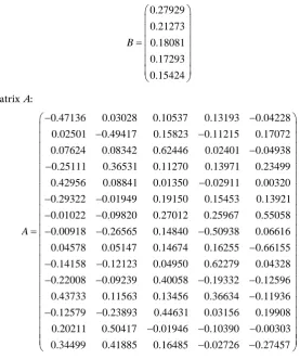
Next, each column of the load matrix is divided by the square root of the va-riance of the corresponding principal component, and the coefficient of each principal component is obtained, and the matrix is denoted as A; then the va-riance matrix is normalized, which are the Weights of each principal compo-nent, this is regarded as matrix B.

DOI: 10.4236/ajibm.2019.911136 2072 American Journal of Industrial and Business Management

Table 3. KMO and Bartley test.

KMO Sampling suitability 0.613

Bartlett’s sphericity test Chi-square obtained last time 304.631

Degree of freedom 105

Significant 0.000

Table 4. Total variance interpretation.

NO

Initial eigenvalue Extracting the sum of squared loads Sum of squared rotational loads

Total Percentage _{of variance} Cumulative % Total _{of variance Cumulative % total} Percentage _{of variance} Percentage Cumulative %

1 3.584 23.890 23.890 3.584 23.890 23.890 2.765 18.431 18.431

2 2.002 13.350 37.240 2.002 13.350 37.240 2.106 14.038 32.470

3 1.745 11.634 48.874 1.745 11.634 48.874 1.790 11.933 44.402

4 1.423 9.488 58.362 1.423 9.488 58.362 1.712 11.415 55.817

5 1.145 7.636 65.998 1.145 7.636 65.998 1.527 10.182 65.998

6 0.991 6.610 72.608

7 0.947 6.310 78.918

8 0.707 4.715 83.633

9 0.616 4.104 87.737

10 0.485 3.234 90.972

11 0.383 2.555 93.527

12 0.341 2.273 95.800

13 0.274 1.827 97.627

14 0.213 1.421 99.048

15 0.143 0.952 100.000

Table 5. Component matrix after the rotation.

Risk number Components

1 2 3 4 5

1 −0.784 0.044 0.141 0.173 −0.052

2 0.042 −0.717 0.212 −0.147 0.211

3 0.127 0.121 0.835 0.031 −0.061

4 −0.418 0.530 0.151 0.183 0.290

5 0.714 0.128 0.018 −0.038 0.004

6 −0.488 −0.028 0.256 0.202 0.172

7 −0.017 −0.143 0.361 0.340 0.680

8 −0.015 −0.386 0.199 −0.666 0.082

9 0.076 0.075 0.196 0.213 −0.817

10 −0.235 −0.176 0.066 0.815 0.053

11 −0.366 −0.134 0.536 −0.253 −0.156

12 0.727 0.168 0.180 0.479 −0.147

13 −0.209 −0.347 0.597 0.041 0.246

14 0.336 0.732 −0.026 −0.136 −0.004

DOI: 10.4236/ajibm.2019.911136 2073 American Journal of Industrial and Business Management

Table 6. Coefficients with coefficients greater than 0.6 in the load matrix.

1 2 3 4 5 6 7 8 9 10 11 12 13 14 15

F1 −0.784 0.042 0.127 −0.418 0.714 −0.488 −0.017 −0.015 0.076 −0.235 −0.366 0.727 −0.209 0.336 0.574

F2 0.044 −0.717 0.121 0.530 0.128 −0.028 −0.143 −0.386 0.075 −0.176 −0.134 0.168 −0.347 0.732 0.608

F3 0.141 0.212 0.835 0.151 0.018 0.256 0.361 0.199 0.196 0.066 0.536 0.180 0.597 −0.026 0.221

F4 0.173 −0.147 0.031 0.183 −0.038 0.202 0.340 −0.666 0.213 0.815 −0.253 0.479 0.041 −0.136 −0.036

F5 −0.052 0.211 −0.061 0.290 0.004 0.172 0.680 0.082 −0.817 0.053 −0.156 −0.147 0.246 −0.004 −0.339

Table 7. 5 main components of national line selection risk.

Main components Names of the main components

F1 Main component of urban modernization

F2 Main component of the political environment

F3 The main component of bilateral cooperation with China

F4 Main component of population development trend

F5 Traffic safety index main component

0.27929 0.21273 0.18081 0.17293 0.15424 B         =        

Matrix A:

0.47136 0.03028 0.10537 0.13193 0.04228 0.02501 0.49417 0.15823 0.11215 0.17072 0.07624 0.08342 0.62446 0.02401 0.04938 0.25111 0.36531 0.11270 0.13971 0.23499 0.42956 0.08841 0.01350 0.02911 0.00320 0.29322 0.01949 A − − − − − = − − −

− 0.19150 0.15453 0.13921

0.01022 0.09820 0.27012 0.25967 0.55058 0.00918 0.26565 0.14840 0.50938 0.06616 0.04578 0.05147 0.14674 0.16255 0.66155 0.14158 0.12123 0.04950 0.62279 0.04328 0.22008 0.09239 0.40058 0.19332

− −

− − −

−

− −

− − − 0.12596

0.43733 0.11563 0.13456 0.36634 0.11936 0.12579 0.23893 0.44631 0.03156 0.19908 0.20211 0.50417 0.01946 0.10390 0.00303 0.34499 0.41885 0.16485 0.02726 0.27457

− − − − − − − − −                                                

Let the data after standardization be matrix X, then the composite score of the sample countrie: S= × ×X A B.

DOI: 10.4236/ajibm.2019.911136 2074 American Journal of Industrial and Business Management lower than the average. Since this score does not intuitively judge the country’s risk, it is converted into a familiar percentage system score [8].

Suppose:

( )

_{( )}

1 exp

M f S

S

= =

+ −

Then control the score between (0,1), then suppose: 60 40

R=M× +

The score can be converted to a percentile, as shown in Table 8:

Table 8. Risk percentage scores and rankings of each country.

Nations Score Ranking Nation Score Ranking

Korea 90.12 1 Albania 70.12 33

Qatar 87.87 2 Macedonia 69.52 34

Oman 85.98 3 Indonesia 69.43 35

Singapore 85.20 4 Belarus 69.12 36

United Arab Emirates 83.99 5 Bosnia 68.82 37

Kuwait 83.41 6 Turkmenistan 68.79 38

Brunei 83.38 7 Georgia 68.54 39

Malaysia 83.36 8 Bhutan 68.18 40

Saudi Arabia 83.17 9 Serbia 68.06 41

South Africa 79.54 10 Romania 66.94 42

Jordan 79.42 11 Turkey 66.52 43

Thailand 77.55 12 Azerbaijan 65.92 44

Latvia 76.13 13 Iraq 64.21 45

Croatia 76.01 14 Kyrgyzstan 63.77 46

Czech Republic 75.95 15 Moldova 63.62 47

Israel 75.52 16 Laos 63.14 48

Russian 74.66 17 Maldives 62.80 49

Iran 74.27 18 Philippines 61.26 50

Bahrain 73.79 19 Egypt 60.43 51

Kazakhstan 73.72 20 Sri Lanka 59.59 52

Bulgaria 73.71 21 East Timor 58.62 53

Lithuania 73.67 22 Pakistan 58.33 54

Poland 73.34 23 Ukraine 58.25 55

Slovenia 73.28 24 Uzbekistan 57.17 56

Estonia 73.09 25 Nepal 57.14 57

Montenegro 72.97 26 Cambodia 56.35 58

Lebanon 72.78 27 Tajikistan 56.08 59

Slovakia 71.97 28 India 54.56 60

Vietnam 71.79 29 Myanmar 54.43 61

Armenia 71.61 30 Bangladesh 53.84 62

Hungary 71.41 31 Afghanistan 52.02 63

DOI: 10.4236/ajibm.2019.911136 2075 American Journal of Industrial and Business Management

3.3. Line Selection Scheme [9]-[13]

In response to the planned plan for the passage of the Asia-Europe Railway, ex-perts proposed several planning options, of which the two most important pro-grams in the Middle East [9] (Figure 1 from China Map Network [4]) are:

1) Channel plan one: China-Kyrgyzstan-Tajikistan-Afghanistan-Iran, finally arrived in Germany;

2) Channel plan two: China-Kazakhstan-Kyrgyzstan-Uzbekistan-Turkmenistan- Iran, finally arrived in Germany.

According to the risk score rankings in Table 8, it can be seen that in the plan 1, Tajikistan and Afghanistan rank at the bottom, while in the plan 2, although Uzbekistan and Kyrgyzstan are ranked lower. However, compared with the plan 1, the advantages are obvious; the total score of the country of plan 2 is much higher than that of plan 1, so the plan 2 was chosen as the Middle East connec-tivity scheme.

4. Conclusions

This paper studies the macro-level risk assessment and line selection of overseas railways based on Principal Component Analysis (PCA). Through the analysis of principal component characteristics, the original 15 risk indicators are reduced in dimension reduction, and five principal components that can represent the main risk factors are obtained. The scores of the load weights of the five principal

DOI: 10.4236/ajibm.2019.911136 2076 American Journal of Industrial and Business Management components are calculated by each country, and the scores are calculated. The risk score is specified, and then through the ranking order, the risk level of the candidate line can be quickly and clearly determined, and the corresponding line selection result is obtained.

The principal component analysis method can be determined from the size of the information sample and the system effect of the sample included in the indi-cator, avoiding the arbitrariness of the expert scoring and subjective judgment, and the risk rankings of each country can be visually seen through the results. All these indicate that this is a more practical method for railway risk assessment and route selection.

This article lacks a control experiment and will use other risk assessment me-thods in subsequent studies to compare the results with principal component analysis to further determine the accuracy of the method.

Acknowledgements

This study is supported in part by China Railway Eryuan Engineering Group Co., Ltd Scientific Research Project (NO. KYY2017069 (17-17)); Sichuan Provincial Science and Technology Support Project (NO. 2019JDRC0133); 2017-2019 Young Elite Scientist Sponsorship Program by CAST (YESS); 2018 Sichuan Provincial Ten Thousand Program Project.

Data Availability

The data used to support the findings of this study are available from the cor-responding author upon request.

Conflicts of Interest

The authors declare no conflicts of interest regarding the publication of this pa-per.

References

[1] Zhu, Y. (2009) Innovation and Practice on Railway Location Concept. Journal of Railway Engineering Society, 26, 1-5.

[2] Liu, W.M. (2002) Research on Main Engineering Economics Problems of Chinese High-Speed Passenger-Only Guided Transport System. Southwest Jiaotong Univer-sity, Chengdu.

[3] Yang, H. (2013) The Application of Clustering Analysis Based on SPSS in Industry Statistical Data. Jilin University, Changchun.

[4] Jin, J. (2019) Research on Risk Evaluation of International Railway Corridors Con-struction among Countries along “The Belt and Road”. China Academy of Railway Sciences, Beijing.

[5] Jia, R.N. (2015) The Study on the Country Risk Assessment and Control Based on Bank. University of International Business and Economics, Beijing.

DOI: 10.4236/ajibm.2019.911136 2077 American Journal of Industrial and Business Management 60-66.

[7] Huang, A., Yang, L.A. and Du, T. (2014) Comprehensive Assessment of Soil Nu-trients Based on PCA. Arid Zone Research, 31, 819-825.

[8] Chen, P. (2014) Principal Component Analysis and Its Application in Feature Ex-traction. Shanxi Normal University, Xi’an.

[9] Cui, Y.P. and Wu, J.Y. (2017) Study on Increasing Operation Quality of China Railway Express by Using Asia-Europe Railway Transpor Corridor. Railway Trans-port and Economy, 39, 68-72.

[10] Yang, C.W., Li, Z.H., Guo X.Y., Yu, W.Y., Jin, J. and Zhu, L. (2019) Application of BP Neural Network Model in Risk Evaluation of Railway Construction. Complexity, 2019, Article ID: 2946158. https://doi.org/10.1155/2019/2946158

[11] Jin, J., Li, Z.H., Zhu, L. and Yang, C.W. (2019) A Research on Risk Assessment of China Railway “Go-Global” Project Construction. Railway Transport and Economy, 41, 86-91.

[12] Jin, J., Zhu, L., Li, Z.H., Tong X.H. and Yang, C.W. (2019) Application of Variable Structure of BPNN in Risk Evaluation of Overseas Railway Construction in Target Countries. Journal of the China Railway Society, 40, 7-12.