Climate: observations, projections and impacts

Climate: Observations,

projections and impacts:

South Korea

Met Office

Simon N. Gosling, University of Nottingham Robert Dunn, Met Office

Fiona Carrol, Met Office Nikos Christidis, Met Office John Fullwood, Met Office Diogo de Gusmao, Met Office Nicola Golding, Met Office Lizzie Good, Met Office Trish Hall, Met Office Lizzie Kendon, Met Office John Kennedy, Met Office Kirsty Lewis, Met Office Rachel McCarthy, Met Office Carol McSweeney, Met Office Colin Morice, Met Office David Parker, Met Office Matthew Perry, Met Office Peter Stott, Met Office Kate Willett, Met Office

Myles Allen, University of Oxford

Nigel Arnell, Walker Institute, University of Reading Dan Bernie, Met Office

Richard Betts, Met Office

Niel Bowerman, Centre for Ecology and Hydrology Bastiaan Brak, University of Leeds

John Caesar, Met Office

Andy Challinor, University of Leeds Rutger Dankers, Met Office Fiona Hewer, Fiona's Red Kite

Chris Huntingford, Centre for Ecology and Hydrology Alan Jenkins, Centre for Ecology and Hydrology

Nick Klingaman, Walker Institute, University of Reading Kirsty Lewis, Met Office

Ben Lloyd-Hughes, Walker Institute, University of Reading Jason Lowe, Met Office

Rachel McCarthy, Met Office

James Miller, Centre for Ecology and Hydrology Robert Nicholls, University of Southampton

Maria Noguer, Walker Institute, University of Reading Friedreike Otto, Centre for Ecology and Hydrology Paul van der Linden, Met Office

Rachel Warren, University of East Anglia

The country reports were written by a range of climate researchers, chosen for their subject expertise, who were drawn from institutes across the UK. Authors from the Met Office and the University of Nottingham collated the contributions in to a coherent narrative which was then reviewed. The authors and

Developed at the request of:

Research conducted by:

We have reached a critical year in our response to climate change. The decisions that we made in Cancún put the UNFCCC process back on track, saw us agree to limit temperature rise to 2 °C and set us in the right direction for reaching a climate change deal to achieve this. However, we still have considerable work to do and I believe that key economies and major emitters have a leadership role in ensuring a successful outcome in Durban and beyond.

To help us articulate a meaningful response to climate change, I believe that it is important to have a robust scientific assessment of the likely impacts on individual countries across the globe. This report demonstrates that the risks of a changing climate are wide-ranging and that no country will be left untouched by climate change.

I thank the UK’s Met Office Hadley Centre for their hard work in putting together such a comprehensive piece of work. I also thank the scientists and officials from the countries included in this project for their interest and valuable advice in putting it together. I hope this report will inform this key debate on one of the greatest threats to humanity.

The Rt Hon. Chris Huhne MP, Secretary of State for Energy and Climate Change

There is already strong scientific evidence that the climate has changed and will continue to change in future in response to human activities. Across the world, this is already being felt as changes to the local weather that people experience every day.

Our ability to provide useful information to help everyone understand how their environment has changed, and plan for future, is improving all the time. But there is still a long way to go. These reports – led by the Met Office Hadley Centre in collaboration with many institutes and scientists around the world – aim to provide useful, up to date and impartial information, based on the best climate science now available. This new scientific material will also contribute to the next assessment from the Intergovernmental Panel on Climate Change.

However, we must also remember that while we can provide a lot of useful information, a great many uncertainties remain. That’s why I have put in place a long-term strategy at the Met Office to work ever more closely with scientists across the world. Together, we’ll look for ways to combine more and better observations of the real world with improved computer models of the weather and climate; which, over time, will lead to even more detailed and confident advice being issued.

Introduction

Understanding the potential impacts of climate change is essential for informing both adaptation strategies and actions to avoid dangerous levels of climate change. A range of valuable national studies have been carried out and published, and the Intergovernmental Panel on Climate Change (IPCC) has collated and reported impacts at the global and regional scales. But assessing the amount of information about past climate change and its future impacts has been available at

Each report contains:

data on extreme events.

Fourth Assessment Report from the IPCC.

Dangerous Climate Change programme (AVOID) and supporting literature.

1

Summary

Climate observations

There has been widespread warming over the Republic of Korea since 1960.

Between 1960 and 2003, warm days and nights have become more frequent while cool days and nights have become less frequent across the region.

There has been a general increase in summer temperatures averaged over the country as a result of human influence on climate, making the occurrence of warm summer temperatures more frequent and cold summer temperatures less frequent.

There is some evidence for a decrease in consecutive dry spell length and an

increase in annual precipitation total between 1960 and 2003, but uncertainties in this increase are large.

Climate change projections

For the A1B emissions scenario projected temperature changes from CMIP3 over the Republic of Korea show increases of up to around 3-3.5°C. There is good agreement between the models in the ensemble.

The Republic of Korea lies at the south of the widespread region across Eastern Asia where projected precipitation shows increases of 10-20% with good agreement across the CMIP3 ensemble.

Climate change impacts projections

Crop yields

2

National-scale assessments agree with the global view of a decline in rice yields towards the end of the century in the Republic of Korea.

Brassicas and other vegetable crops constitute an important part of the country’s agricultural production but crop yield changes are uncertain as these crops are not routinely included in climate change impact assessments.

Food security

The Republic of Korea is currently a country with extremely low levels of undernourishment.

The majority of global studies included here suggest that Republic of Korea will not face serious food security issues over the next 40 years. However, further research is needed to address knowledge gaps in projections of food security for the country.

Water stress and drought

Global-scale studies included here indicate that the Republic of Korea currently suffers from a moderate to high level of water stress, and some project that water stress in the country could increase with climate change. However, uncertainty is high owing to the level of understanding about how the monsoon may be affected by climate change.

Pluvial flooding and rainfall

The IPCC AR4 noted that mean and extreme precipitation for Korea was projected to increase with climate change, with stronger precipitation increases during the summer season.

Recent studies support this, with increases in precipitation noted in a majority of the studies considered for both historic observations and future climate projections.

Fluvial flooding

Climate change impact studies for the Republic of Korea have produced very different projections of future changes in flooding, even when the study area is the same, because of different choices of scenarios, models and simulation period.

3

century and in the A1B scenario, with some models projecting very large increases. This is consistent with the results of other global and local studies.

Tropical cyclones

There remains large uncertainty in the current understanding of how tropical cyclones might be affected by climate change. To this end, caution should be applied in

interpreting model-based results, even where the models are in agreement.

Projected change in the intensity of cyclones in the western Pacific basin are

considered more robust than projected change in their frequency. A number of global- and regional-scale studies included here project that cyclone intensity could increase considerably in the future in this basin. These increases in intensity could be greatest for the most severe cyclones, which could lead to large increases in cyclone damages in the Republic of Korea.

Estimates of future cyclone damage in the Republic of Korea are highly uncertain due to the small size of the country and the limited resolutions of the climate models used to simulate shifts in tropical-cyclone tracks under climate change.

Coastal regions

Two recent global assessments of the impact of sea level rise on coastal regions, suggest that climate change could have major implications for the Republic of Korea’s coastal populations.

However, the magnitude of the projected impacts differs between the two assessments because of different methodological approaches.

One of the studies shows that around 50% of the coastal population (around 863,000 people) could be affected by a 10% intensification of the current 1-in-100-year storm surge combined with a prescribed 1m SLR.

5

Table of Contents

Chapter 1 – Climate Observations

Rationale ... 10

Climate overview ... 12

Analysis of long-term features in the mean temperature ... 13

Temperature extremes ... 15

Recent extreme temperature events ... 15

Severe heat wave, July-August 1994 ... 15

Analysis of long-term features in moderate temperature extremes ... 16

Attribution of changes in likelihood of occurrence of seasonal mean temperatures ... 22

Summer 1994 ... 22

Precipitation extremes ... 24

Recent extreme precipitation events ... 25

Drought, March-May 2001 ... 25

Flooding, July 2006 ... 25

Analysis of long-term features in precipitation ... 25

Storms ... 28

Recent storm events ... 29

Typhoon Maemi, September 2003 ... 29

Typhoon Kompasu, September 2010 ... 29

Summary ... 30

The main features seen in observed climate over the Republic of Korea from this analysis are: ... 30

Methodology annex ... 31

Recent, notable extremes ... 31

Observational record ... 32

Analysis of seasonal mean temperature ... 32

Analysis of temperature and precipitation extremes using indices ... 33

Presentation of extremes of temperature and precipitation ... 43

Attribution ... 47

References ... 50

Acknowledgements ... 54

Chapter 2 – Climate Change Projections

Introduction ... 56

Climate projections ... 58

Summary of temperature change in the Republic of Korea ... 60

Summary of precipitation change in the Republic of Korea ... 60

Chapter 3 – Climate Change Impact Projections

Introduction ... 62

Aims and approach ... 62

6

Supporting literature ... 63

AVOID programme results ... 64

Uncertainty in climate change impact assessment ... 64

Summary of findings for each sector ... 69

Crop yields ... 72

Headline... 72

Supporting literature ... 72

Introduction ... 72

Assessments that include a global or regional perspective ... 74

National-scale or sub-national scale assessments ... 78

AVOID programme results ... 79

Methodology ... 79

Results ... 80

Food security ... 82

Headline... 82

Introduction ... 82

Assessments that include a global or regional perspective ... 82

National-scale or sub-national scale assessments ... 88

Water stress and drought ... 89

Headline... 89

Introduction ... 89

Assessments that include a global or regional perspective ... 90

National-scale or sub-national scale assessments ... 94

AVOID Programme Results ... 94

Methodology ... 94

Results ... 95

Pluvial flooding and rainfall ... 97

Headline... 97

Introduction ... 97

Assessments that include a global or regional perspective ... 97

National-scale or sub-national scale assessments ... 98

Fluvial flooding ... 100

Headline... 100

Supporting literature ... 100

Introduction ... 100

Assessments that include a global or regional perspective ... 101

National-scale or sub-national scale assessments ... 102

AVOID Programme results ... 103

Methodology ... 104

Results ... 104

Tropical cyclones ... 106

Headline... 106

Introduction ... 106

7

National-scale or sub-national scale assessments ... 112

Coastal regions ... 113

Headline... 113

Assessments that include a global or regional perspective ... 113

National-scale or sub-national scale assessments ... 121

9

10

Rationale

Present day weather and climate play a fundamental role in the day to day running of society. Seasonal phenomena may be advantageous and depended upon for sectors such as farming or tourism. Other events, especially extreme ones, can sometimes have serious negative impacts posing risks to life and infrastructure and significant cost to the economy. Understanding the frequency and magnitude of these phenomena, when they pose risks or when they can be advantageous and for which sectors of society, can significantly improve societal resilience. In a changing climate it is highly valuable to understand possible future changes in both potentially hazardous events

and those reoccurring seasonal events that are depended upon by sectors such as agriculture and tourism. However, in order to put potential future changes in context, the present day must first be well understood both in terms of common seasonal phenomena and extremes.

The purpose of this chapter is to summarise the weather and climate from 1960 to present day. This begins with a general climate overview including an up to date analysis of changes in surface mean temperature. These changes may be the result of a number of factors including climate change, natural variability and changes in land use. There is then a focus on extremes of temperature, precipitation and storms selected from 1994 onwards, reported in the World Meteorological Organization (WMO) Annual Statement on the Status of the Global Climate and/or the Bulletin of the American Meteorological Society (BAMS) State of the Climate reports. This is followed by a discussion of changes in moderate extremes from 1960 onwards using the HadEX extremes database (Alexander et al. 2006) which

categorises extremes of temperature and precipitation. These are core climate variables which have received significant effort from the climate research community in terms of data acquisition and processing and for which it is possible to produce long high quality records for monitoring. No new analysis is included for storms (see the methodology annex that follows for background). For seasonal temperature extremes, an attribution analysis then puts the seasons with highlighted extreme events into context of the recent climate versus a hypothetical climate in the absence of anthropogenic emissions (Christidis et al, 2011). It is

11

important to note that we carry out our attribution analyses on seasonal mean temperatures over the entire country. Therefore these analyses do not attempt to attribute the changed likelihood of individual extreme events. The relationship between extreme events and the

large scale mean temperature is likely to be complex, potentially being influenced by inter

alia circulation changes, a greater expression of natural internal variability at smaller scales,

and local processes and feedbacks. Attribution of individual extreme events is an area of developing science. The work presented here is the foundation of future plans to

systematically address the region’s present and projected future weather and climate, and the associated impacts.

The methodology annex provides details of the data shown here and of the scientific

12

Climate overview

The Republic of Korea is a peninsula extending southwards from 38°N to 34°N on the eastern seaboard of Asia and connected, via North Korea, to north-eastern China. On account of this proximity to the vast land mass of Asia the climate has quite continental characteristics, despite the country being a peninsula, with a 22-28°C difference between mid-winter and mid-summer mean temperature. The country’s climate is governed by the ‘Asiatic Monsoon’ which, in summer, draws warm moist winds across the peninsula from the Pacific Ocean towards low atmospheric pressure that develops over the hot Asian interior. However, in winter, winds from between north and west blow outwards from the huge high atmospheric pressure system that develops over Siberia.

Despite the winter Siberian air mass having very cold, dry and cloudless characteristics, over the Republic of Korea it regularly interacts with eastward-moving frontal weather systems bringing snowfalls and occasional thaws with rain. Winter precipitation is typically around 20-80 mm per month, much of it falling as snow. Temperatures decrease from south to north so that the average number of days on which snow falls increases from 10 in the far south to 28 in the north. Mean January temperature is around 3°C at Busan in the south, where the average daytime maximum is 7°C falling to -1°C at night, but only around -2°C at Seoul in the north where the average daytime maximum is 2°C falling to -6°C at night. A quick

transition from the winter weather type to the summer weather type occurs in April/early May and vice-versa in late October/early November.

Summers are very warm and wet. Under maritime influence, the warmest month is delayed to August, when the mean temperature is around 26°C throughout the country, with daily maxima typically around 29°C, falling only to around 23°C at night. Most of the annual precipitation occurs between June and September when monthly totals range typically between 100 and 350 mm. Annual average precipitation is 1344mm at Seoul and 1492mm at Busan.

13

Analysis of long-term features in the mean temperature

CRUTEM3 data (Brohan et al., 2006) have been used to provide an analysis of mean temperatures from 1960 to 2010 over the Republic of Korea using the median of pairwise slopes method to fit the trend (Sen, 1968; Lanzante, 1996). The methods are fully described in the methodology annex. In concert with increasing global average temperatures

14

15

Temperature extremes

Both hot and cold temperature extremes can place many demands on society. While seasonal changes in temperature are normal and indeed important for a number of societal sectors (e.g. tourism, farming etc.), extreme heat or cold can have serious negative impacts. Importantly, what is ‘normal’ for one region may be extreme for another region that is less well adapted to such temperatures.

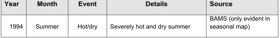
Very few extreme temperature events have been reported in recent years in the Republic of Korea. Table 1 shows an extreme temperature event that is reported in WMO Statements on Status of the Global Climate and/or BAMS State of the Climate reports. This event, a heat wave in July and August 1994, is highlighted below as an example of an extreme

temperature event that affected the Republic of Korea.

Year Month Event Details Source

1994 Summer Hot/dry Severely hot and dry summer

BAMS (only evident in seasonal map)

Table 1. Selected extreme temperature event reported in WMO Statements on Status of the Global Climate and/or BAMS State of the Climate reports since 1994.

Recent extreme temperature events

Severe heat wave, July-August 1994

The heat wave that occurred during July and August, 1994, was ranked among the worst weather related disasters in East Asia. It was by far the longest and most severe heat wave

observed over the Korean Peninsula since 1942, and possibly in the entire 20th _century

(Choi, 2004). It lasted 29 days in total in Seoul, and the highest daily maximum temperature

reached 39.4˚C (daily mean temperature was 33.1 ˚C). The total death toll exceeded 3000,

16

The weather conditions during this event, as well as the severity of impacts on human life were extremely rare, but there is some evidence that the probability of recurrence of an event such as this is sharply rising due to gradual warming of the climate (Kysely & Kim, 2009).

Analysis of long-term features in moderate temperature

extremes

HadEX extremes indices (Alexander et al. 2006) are used here for the Republic of Korea from 1960 to 2003 using daily maximum and minimum temperatures. Here we discuss changes in the frequency of cool days and nights and warm days and nights which are moderate extremes. Cool days/nights are defined as being below the 10th percentile of daily maximum/minimum temperature and warm days/nights are defined as being above the 90th percentile of the daily maximum/minimum temperature. The methods are fully described in the methodology annex.

Between 1960 and 2003, in concert with increasing mean temperature, warm days and nights have become more frequent while cool days and nights have become less frequent across the region with higher confidence. This is consistent with previous research (Jung et al. 2002; Ryoo et al. 2004). The data presented here are annual totals, averaged across all seasons, and so direct interpretation in terms of summer heat waves and winter cool snaps is not possible. Due to the land-sea mask used, the Republic of Korea is represented by a single grid box.

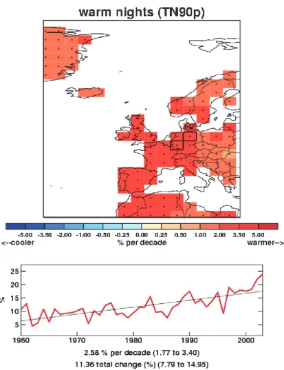
Night time temperatures (daily minima) show a widespread positive shift in the distribution with fewer cool nights and more warm nights. Confidence is high throughout (Figure 3 a,b,c,d). Regional averages show higher confidence signals of fewer cool nights and more warm nights.

17

21

Figure 3. Percentage change in cool nights (a,b), warm nights (c,d), cool days (e,f) and warm days (g,h) for the Republic of Korea over the period 1960 to 2003 relative to 1961-1990 from HadEX (Alexander et al. 2006). a,c,e,g) Grid box decadal trends. Grid boxes outlined in solid black contain at least 3 stations and so are likely to be more representative of the wider grid box. Trends are fitted using the median of pairwise slopes method (Sen 1968, Lanzante 1996). Higher confidence in a long-term trend is shown by a black dot if the 5th _{to 95}th _{percentile slopes are of the same sign. Differences}

in spatial coverage occur because each index has its own decorrelation length scale (see

methodology annex). b,d,f,h) Area averaged annual time series for 125.625 to 129.375 o E, 33.75 to 38.75 o N as shown in the red box in Figure 1. Trends are fitted as described above. The decadal trend and its 5th _{to 95}th _{percentile pairwise slopes are shown as well as the change over the period for}

22

Attribution of changes in likelihood of occurrence of

seasonal mean temperatures

Today’s climate covers a range of likely extremes. Recent research has shown that the temperature distribution of seasonal means would likely be different in the absence of anthropogenic emissions (Christidis et al., 2011). Here we discuss the seasonal means, within which the highlighted extreme temperature events occur, in the context of recent climate and the influence of anthropogenic emissions on that climate. The methods are fully described in the methodology annex.

Summer 1994

23

Figure 4. Distributions of the June-July-August mean temperature anomalies (relative to 1961-1990) averaged over an East Asian region that encompasses the Republic of Korea (122-150E, 30-48N) including (red lines) and excluding (green lines) the influence of anthropogenic forcings. The

24

Precipitation extremes

Precipitation extremes, either excess or deficit, can be hazardous to human health, societal infrastructure, and livestock and agriculture. While seasonal fluctuations in precipitation are normal and indeed important for a number of societal sectors (e.g. tourism, farming etc.), flooding or drought can have serious negative impacts. These are complex phenomena and often the result of accumulated excesses or deficits or other compounding factors such as spring snow-melt, high tides/storm surges or changes in land use. The analysis section below deals purely with precipitation amounts.

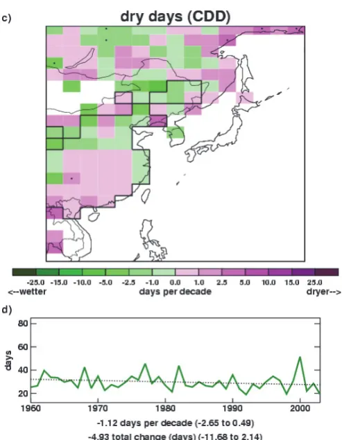
Table 2 shows selected extreme events since 2000 that are reported in WMO Statements on Status of the Global Climate and/or BAMS State of the Climate reports. Two events, the March-May drought of 2001 and flooding during July 2006, are highlighted below as examples of recent extreme precipitation events that affected the Republic of Korea.

Year Month

Event

Details

Source

2000 Aug-Sep Wet

Typhoon Prapiroon struck the west coast of the Korean Peninsula bringing heavy rainfall

and flash floods. WMO (2001)

2001 Mar-May Drought Severe drought WMO (2002)

2006 Jul Flooding

Locations record more than 500 mm of rainfall in a few days.

BAMS (Bell & Halpert, 2007))

25

Recent extreme precipitation events

Drought, March-May 2001

Abnormally strong drought conditions hit the Korean Peninsula in 2001 (Min et al., 2003; Kang and Byun, 2001). The severity of this drought is illustrated by Figure 82 of Waple et al. (2002). During three months of drought, the Republic of Korea received only about 30 percent of the average rainfall it usually receives during the crucial spring planting season and the country’s agriculture was particularly affected.

Flooding, July 2006

Heavy rains in July 2006 affected several provinces of the Republic of Korea, especially the mountainous Gangwon Province where some locations recorded more than 500 millimetres of rain in just a few days. However, the heavy rains were not sufficiently widespread and persistent to be evident on the rainfall map for June to August 2006 in Figure 7.5 of Bell and Halpert (2007) which indicates near-normal seasonal totals over the Republic of Korea.

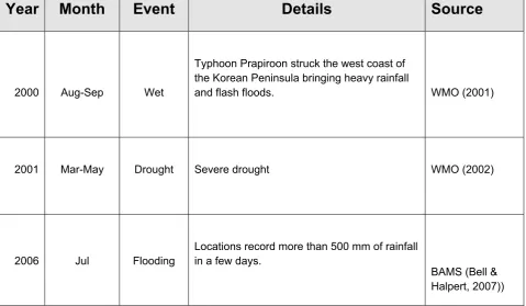
Analysis of long-term features in precipitation

HadEX extremes indices (Alexander et al. 2006) are used here for the Republic of Korea from 1960 to 2003 using daily precipitation totals. Here we discuss changes in the annual total precipitation, and in the frequency of prolonged (greater than 6 days) dry spells. The

methods are fully described in the methodology annex.

27

Figure 5. Change in total annual precipitation (a, b) and continuous dry spell length (c,d) for the Republic of Korea over the period 1960 to 2003 using a base reference period of 1961-1990 from HadEX (Alexander et al. 2006). a,c) Decadal trends as described in Figure 3. b,d) Area average annual time-series for 125.625 to 129.375 o _{E, 33.75 to 38.75} o _{N as described in Figure 3. All the}

28

Storms

Storms can be very hazardous to all sectors of society. They can be small with localised impacts or spread across multiple states. There is no systematic observational analysis included for storms because, despite recent progress (Peterson et al. 2011; Cornes and Jones 2011), wind data are not yet adequate for worldwide robust analysis (see the methodology annex). Further progress awaits studies of the more reliable barometric pressure data through the new 20th Century Reanalysis (Compo et al., 2011) and its planned successors.

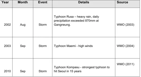
Table 3 shows selected extreme events since 2000 that are reported in WMO Statements on Status of the Global Climate and/or BAMS State of the Climate reports. Two events,

Typhoon Maemi in September 2003 and Typhoon Kompasu in 2010, are highlighted below as examples of recent storm events that affected the Republic of Korea.

Year Month Event Details Source

2002 Aug Storm

Typhoon Rusa – heavy rain, daily precipitation exceeded 870mm at

Gangneung. WMO (2003)

2003 Sep Storm Typhoon Maemi - high winds WMO (2004)

2010 Sep Storm

Typhoon Kompasu - strongest typhoon to hit Seoul in 15 years

WMO (2011)

29

Recent storm events

Typhoon Maemi, September 2003

Super-typhoon Maemi caused widespread destruction in the Republic of Korea. Maemi formed east of the Philippines and moved northwest-ward while intensifying, reaching its maximum intensity near Okinawa, Japan, and weakened before making landfall in the Republic of Korea. High winds and rainfall associated with Maemi were responsible for more than 100 deaths and destroyed more than 1.4 million houses, damaged roads and bridges, and sank at least 82 vessels (Camargo, 2004).

Typhoon Kompasu, September 2010

Typhoon Kompasu moved over the southern islands of Japan and the west coast of the

Korean Peninsula before striking the Seoul Metropolitan Area on 2nd _{September 2010.}

30

Summary

The main features seen in observed climate over the Republic of Korea from this analysis are:

There has been widespread warming over the Republic of Korea since 1960. Between 1960 and 2003, warm days and nights have become more frequent while

cool days and nights have become less frequent across the region.

There has been a general increase in summer temperatures averaged over the country as a result of human influence on climate, making the occurrence of warm summer temperatures more frequent and cold summer temperatures less frequent. There is some evidence for a decrease in consecutive dry spell length and an

31

Methodology annex

Recent, notable extremes

In order to identify what is meant by ‘recent’ events the authors have used the period since 1994, when WMO Status of the Global Climate statements were available to the authors. However, where possible, the most notable events during the last 10 years have been chosen as these are most widely reported in the media, remain closest to the forefront of the memory of the country affected, and provide an example likely to be most relevant to today’s society. By ‘notable’ the authors mean any event which has had significant impact either in terms of cost to the economy, loss of life, or displacement and long term impact on the population. In most cases the events of largest impact on the population have been chosen, however this is not always the case.

Tables of recent, notable extreme events have been provided for each country. These have been compiled using data from the World Meteorological Organisation (WMO) Annual Statements on the Status of the Global Climate. This is a yearly report which includes contributions from all the member countries, and therefore represents a global overview of events that have had importance on a national scale. The report does not claim to capture all events of significance, and consistency across the years of records available is variable. However, this database provides a concise yet broad account of extreme events per country. This data is then supplemented with accounts from the monthly National Oceanic and

Atmospheric Administration (NOAA) State of the Climate reports which outline global extreme events of meteorological significance.

32

Our search for data has not been exhaustive given the number of countries and events included. Although there are a wide variety of sources available, for many events, an official account is not available. Therefore figures given are illustrative of the magnitude of impact only (references are included for further information on sources). It is also apparent that the reporting of extreme events varies widely by region, and we have, where possible, engaged with local scientists to better understand the impact of such events.

The aim of the narrative for each country is to provide a picture of the social and economic vulnerability to the current climate. Examples given may illustrate the impact that any given extreme event may have and the recovery of a country from such an event. This will be important when considering the current trends in climate extremes, and also when examining projected trends in climate over the next century.

Observational record

In this section we outline the data sources which were incorporated into the analysis, the quality control procedure used, and the choices made in the data presentation. As this report is global in scope, including 23 countries, it is important to maintain consistency of

methodological approach across the board. For this reason, although detailed datasets of extreme temperatures, precipitation and storm events exist for various countries, it was not possible to obtain and incorporate such a varied mix of data within the timeframe of this project. Attempts were made to obtain regional daily temperature and precipitation data from known contacts within various countries with which to update existing global extremes databases. No analysis of changes in storminess is included as there is no robust historical analysis of global land surface winds or storminess currently available.

Analysis of seasonal mean temperature

33

their median. This is a robust estimator of the slope which is not sensitive to outlying points.

High confidence is assigned to any trend value for which the 5th _{to 95}th _{percentiles of the}

pairwise slopes are of the same sign as the trend value and thus inconsistent with a zero trend.

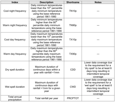
Analysis of temperature and precipitation extremes using indices

In order to study extremes of climate a number of indices have been created to highlight different aspects of severe weather. The set of indices used are those from the World Climate Research Programme (WCRP) Climate Variability and Predictability (CLIVAR) Expert Team on Climate Change Detection and Indices (ETCCDI). These 27 indices use daily rainfall and maximum and minimum temperature data to find the annual (and for a subset of the indices, monthly) values for, e.g., the ‘warm’ days where daily maximum

temperature exceeds the 90th _{percentile maximum temperature as defined over a 1961 to}

34

Index Description Shortname Notes

Cool night frequency

Daily minimum temperatures lower than the 10th percentile daily minimum temperature

using the base reference period 1961-1990

TN10p ---

Warm night frequency

Daily minimum temperatures higher than the 90th percentile daily minimum temperature using the base reference period 1961-1990

TN90p ---

Cool day frequency

Daily maximum temperatures lower than the 10th percentile daily maximum temperature

using the base reference period 1961-1990

TX10p ---

Warm day frequency

Daily maximum temperatures higher than the 90th percentile daily maximum temperature using the base reference period 1961-1990

TX90p ---

Dry spell duration continuous days within a Maximum duration of

year with rainfall <1mm CDD

Lower data coverage due to the requirement for a ‘dry spell’ to be at least 6

days long resulting in intermittent temporal

coverage

Wet spell duration

Maximum duration of continuous days with rainfall >1mm for a given

year

CWD

Lower data coverage due to the requirement for a ‘wet spell’ to be at least 6

days long resulting in intermittent temporal

coverage Total annual

precipitation Total rainfall per year PRCPTOT ---

Table 4. Description of ETCCDI indices used in this document.

A previous global study of the change in these indices, containing data from 1951-2003 can be found in Alexander et al. 2006, (HadEX; see http://www.metoffice.gov.uk/hadobs/hadex/). In this work we aimed to update this analysis to the present day where possible, using the most recently available data. A subset of the indices is used here because they are most easily related to extreme climate events (Table 4).

Use of HadEX for analysis of extremes

The HadEX dataset comprises all 27 ETCCDI indices calculated from station data and then smoothed and gridded onto a 2.5° x 3.75° grid, chosen to match the output from the Hadley Centre suite of climate models. To update the dataset to the present day, indices are calculated from the individual station data using the RClimDex/FClimDex software;

35

Meteorological Service of Canada. Given the timeframe of this project it was not possible to obtain sufficient station data to create updated HadEX indices to present day for a number of countries: Brazil; Egypt; Indonesia; Japan (precipitation only); South Africa; Saudi Arabia; Peru; Turkey; and Kenya. Indices from the original HadEX data-product are used here to show changes in extremes of temperature and precipitation from 1960 to 2003. In some cases the data end prior to 2003. Table 5 summarises the data used for each country. Below, we give a short summary of the methods used to create the HadEX dataset (for a full

description see Alexander et al. 2006).

To account for the uneven spatial coverage when creating the HadEX dataset, the indices for each station were gridded, and a land-sea mask from the HadCM3 model applied. The interpolation method used in the gridding process uses a decorrelation length scale (DLS) to determine which stations can influence the value of a given grid box. This DLS is calculated from the e-folding distance of the individual station correlations. The DLS is calculated separately for five latitude bands, and then linearly interpolated between the bands. There is a noticeable difference in spatial coverage between the indices due to these differences in decorrelation length scales. This means that there will be some grid-box data where in fact there are no stations underlying it. Here we apply black borders to grid-boxes where at least 3 stations are present to denote greater confidence in representation of the wider grid-box area there. The land-sea mask enables the dataset to be used directly for model comparison with output from HadCM3. It does mean, however, that some coastal regions and islands over which one may expect to find a grid-box are in fact empty because they have been treated as sea

Data sources used for updates to the HadEX analysis of extremes

We use a number of different data sources to provide sufficient coverage to update as many countries as possible to present day. These are summarised in Table 5. In building the new datasets we have tried to use exactly the same methodology as was used to create the original HadEX to retain consistency with a product that was created through substantial international effort and widely used, but there are some differences, which are described in the next section.

Wherever new data have been used, the geographical distributions of the trends were compared to those obtained from HadEX, using the same grid size, time span and fitting method. If the pattern of the trends in the temperature or precipitation indices did not match that from HadEX, we used the HadEX data despite its generally shorter time span.

36

stations used to create the gridded results are different from those in HadEX, and the quality control procedures used are also very likely to be different. Countries where we decided to use HadEX data despite the existence of more recent data are Egypt and Turkey.

GHCND:

The Global Historical Climate Network Daily data has near-global coverage. However, to ensure consistency with the HadEX database, the GHCND stations were compared to those stations in HadEX. We selected those stations which are within 1500m of the stations used in the HadEX database and have a high correlation with the HadEX stations. We only took the precipitation data if its r>0.9 and the temperature data if one of its r-values >0.9. In addition, we required at least 5 years of data beyond 2000. These daily data were then

converted to the indices using the fclimdex software.

ECA&D and SACA&D:

The European Climate Assessment and Dataset and the Southeast Asian Climate Assessment and Dataset data are pre-calculated indices comprising the core 27 indices from the ETCCDI as well as some extra ones. We kindly acknowledge the help of Albert

Klein Tank, the KNMI1 _{and the BMKG}2 _{for their assistance in obtaining these data.}

Mexico:

The station data from Mexico has been kindly supplied by the SMN3 _{and Jorge Vazquez.}

These daily data were then converted to the required indices using the Fclimdex software.

There are a total of 5298 Mexican stations in the database. In order to select those which have sufficiently long data records and are likely to be the most reliable ones we performed a cross correlation between all stations. We selected those which had at least 20 years of

data post 1960 and have a correlation with at least one other station with an r-value >0.95.

This resulted in 237 stations being selected for further processing and analysis.

Indian Gridded:

The India Meteorological Department provided daily gridded data (precipitation 1951-2007, temperature 1969-2009) on a 1° x 1° grid. These are the only gridded daily data in our analysis. In order to process these in as similar a way as possible the values for each grid

1_{Koninklijk Nederlands Meteorologisch Instituut – The Royal Netherlands Meteorological Institute}

2

Badan Meteorologi, Klimatologi dan Geofisika – The Indonesian Meteorological, Climatological and Geophysical Agency

3

37

38 Coun tr y Region bo x (re d da she d boxes in Fig. 1 and on each map at begin ning of cha pt er ) Data sour ce (T = temperature, P = precipitation) Period of data cov erage (T = temp erat ure, P = pre cipitati on) Indices inclu ded (se e Tabl e 4 for details)

Temporal resolution av

ailable Not es Argentin a 73.125 to 54. 375 o W, 21.25 to 56 .25 o S Matilde Ru st icu cci (T,P) 1960 -20 10 (T ,P) TN10 p, TN9 0p , TX10p, TX90 p, PRCPT O T, C DD, CW D annu al Aus tralia 114.37 5 to 15 5.625

o E

, 1 1. 25 to 4 3. 75

o S

GHCND (T,P ) 1960 -20 10 (T ,P) TN10 p, TN9 0p , TX10p, TX90 p, PRCPT O T, C DD, CW D monthly, se aso na l a nd annu al Land -sea ma sk has been adapte d to inclu de Ta sm ania an d the area ar ound Brisb ane Banglad esh 88.125 to 91. 875 o E, 21.25 to 26.25 o N Indian Gri dde d data (T,P) 1960 -20 07 (P ), 1970 -20 09 (T ) TN10 p, TN9 0p , TX10p, TX90 p, PRCPT O T, C DD, CW D monthly, se aso na l a nd annu al Interpolate d from India n Gridded da ta Braz il 73.125 to 31. 875 o W, 6.25

o N

to

33.75

o S

HadEX (T,P) 1960 -20 00 (P ) 2002 (T) TN10 p, TN9 0p , TX10p, TX90 p, PRCPT O T, C DD, CW D annu al Spatial cove rage is poor Ch in a 73.125 to 13 3. 125 o E, 21.25 to 53.75 o N GH CN D (T,P ) 1960 -19 97 (P ) 1960 -20 03 (Tmin ) 1960 -20 10 (Tma x ) TN10 p, TN9 0p , TX10p, TX90 p, PRCPT O T, C DD, CW D monthly, se aso na l a nd annu al Preci pitation has very po or covera ge beyond 1997 except in 20 03 -04, an d no data at all in 2000 -02, 20 05 -11 Egypt 24.375 to 35. 625 o E, 21.25 to 31.25 o N HadEX (T,P) No data TN10 p, TN9 0p , TX10p, TX90 p, PRCPT O T, annu al There are no data for Egyp t so all grid -box values ha ve been inte rpolate d from station s in Jo rdan, Israel, Libya and Sudan Fran ce 5.625

o W

to

9

.3

75

o E

, 4 1. 25 to 5 1. 25

o N

39 Germ any 5.625 to 16.8 75

o E,

46.25

to

56.2

5

o N

ECA&D (T,P) 1960 -20 10 (T ,P) TN10 p, TN9 0p , TX10p, TX90 p, PRCPT O T, C DD, CW D monthly, se aso na l a nd annu al India 69.375 to 99. 375 o E, 6.25 to 36.25

o N

Indian Gri dde d data (T,P) 1960 -20 03 (P ), 1970 -20 09 (T ) TN10 p, TN9 0p , TX10p, TX90 p, PRCPT O T, C DD, CW D monthly, se aso na l a nd annu al Indone sia 95.625 to 14 0. 625 o E, 6.25

o N

to

1

1.

25

o S

HadEX (T,P) 1968 -20 03 (T ,P) TN10 p, TN9 0p , TX10p, TX90 p, PRCPT O T, annu al Spatial cove rage is poor Italy 5.625 to 16.8 75

o E,

36.25

to

46.2

5

o N

ECA&D (T,P) 1960 -20 10 (T ,P) TN10 p, TN9 0p , TX10p, TX90 p, PRCPT O T, C DD, CW D monthly, se aso na l a nd annu al Land -sea ma sk has been adapte d to improve cove rage of Italy Ja pa n 129.37 5 to 14 4.375

o E

, 3 1. 25 to 4 6. 25

o N

HadEX (P) GH CN D (T ) 1960 -20 03 (P ) 1960 -20 00 (Tmin ) 1960 -20 10 (Tma x ) TN10 p, TN9 0p , TX10p, TX90 p, PRCPT O T, monthly, se aso na l a nd annu al (T), annu al (P) Kenya 31.875 to 43. 125 o E, 6.25

o N

to 6 .2 5 o S HadEX (T,P) 1960 -19 99 (P ) TN10 p, TN9 0p , TX10p, TX90 p, PRCPT O T annu al There are no temperature data for Kenya and so grid-box valu es have been inte rpol ated from nei ghbo urin g Uga nda and the Unite d Re publi c of Tanzania. Re gional ave rag es in clud e grid -boxe s fro m outside Ke nya that enabl e co ntin uation to 200 3 Mexico 118.12 5 to 88 .125 o W, 13.75 to 33 .75 o N Ra w station data from the Servicio Meteorológi co Na cion al (SMN ) (T,P) 1960 -20 09 (T ,P) TN10 p, TN9 0p , TX10p, TX90 p, PRCPT O T, C DD, CW D monthly, se aso na l a nd annu al 237/52 98 stat ions sele cted. Non uniform spati al coverage. Dro p in T and P covera ge in 2009. Peru 84.735 to 65. 625 o W, 1.25

o N

t

o

18.75

o S

40 Ru ssi a We st Ru ssi a 28.125 to 10 6. 875 o E, 43.75 to 78.75 o N, Ea st R us si a 103.12 5 to 18 9.375

o E

, 4 3. 75 to 7 8. 75

o N

ECA&D (T,P) 1960 -20 10 (T ,P) TN10 p, TN9 0p , TX10p, TX90 p, PRCPT O T, C DD, CW D monthly, se aso na l a nd annu al Cou ntry split for presentatio n purp oses only. Saudi Arabi a 31.875 to 54. 375 o E, 16.25 to 33.75 o N HadEX (T,P) 1960 -20 00 (T ,P) TN10 p, TN9 0p , TX10p, TX90 p, PRCPT O T annu al Spatial cove rage is poor South Africa 13.125 to 35. 625 o W, 21.25 to 36 .25 o S HadEX (T,P) 1960 -20 00 (T ,P) TN10 p, TN9 0p , TX10p, TX90 p, PRCPT O T, C DD, CW D annu al --- Rep ubli c of Korea 125.62 5 to 12 9.375

o E

, 3 3. 75 to 3 8. 75

o N

HadEX (T,P) 1960 -20 03 (T ,P) TN10 p, TN9 0p , TX10p, TX90 p, PR C PTOT, CD D annu al There are too few data poi nts for CWD to calculate trend s or regio nal times eries Spain 9.375

o W

to

1

.8

75

o E

, 3 6. 25 to 4 3. 75

o N

ECA&D (T,P) 1960 -20 10 (T ,P) TN10 p, TN9 0p , TX10p, TX90 p, PRCPT O T, C DD, CW D monthly, se aso na l a nd annu al Turkey 24.375 to 46. 875 o E, 36.25 to 43.75 o N HadEX (T,P) 1960 -20 03 (T ,P) TN10 p, TN9 0p , TX10p, TX90 p, PRCPT O T, C DD, CW D annu al Inter m ittent cover age in CW D and CDD with no re gio nal avera ge beyond 20 00

United _Kingdom

9.375

o W

to

1

.8

75

o E

, 5 1. 25 to 5 8. 75

o N

ECA&D (T,P) 1960 -20 10 (T ,P) TN10 p, TN9 0p , TX10p, TX90 p, PRCPT O T, C DD, CW D monthly, se aso na l a nd annu al

United _States

41

Quality control and gridding procedure used for updates to the HadEX analysis of extremes

In order to perform some basic quality control checks on the index data, we used a two-step process on the indices. Firstly, internal checks were carried out, to remove cases where the 5 day rainfall value is less than the 1 day rainfall value, the minimum T_min is greater than the minimum T_max and the maximum T_min is greater than the maximum T_max. Although these are physically impossible, they could arise from transcription errors when creating the daily dataset, for example, a misplaced minus sign, an extra digit appearing in the record or a column transposition during digitisation. During these tests we also require that there are at least 20 years of data in the period of record for the index for that station, and that some data is found in each decade between 1961 and 1990, to allow a reasonable estimation of the climatology over that period.

Weather conditions are often similar over many tens of kilometres and the indices calculated in this work are even more coherent. The correlation coefficient between each station-pair combination in all the data obtained is calculated for each index (and month where

appropriate), and plotted as a function of the separation. An exponential decay curve is fitted

to the data, and the distance at which this curve has fallen by a factor 1/e is taken as the

decorrelation length scale (DLS). A DLS is calculated for each dataset separately. For the GHCND, a separate DLS is calculated for each hemisphere. We do not force the fitted decay curve to show perfect correlation at zero distance, which is different to the method employed when creating HadEX. For some of the indices in some countries, no clear decay pattern was observed in some data sets or the decay was so slow that no value for the DLS could be determined. In these cases a default value of 200km was used.

We then perform external checks on the index data by comparing the value for each station with that of its neighbours. As the station values are correlated, it is therefore likely that if one station measures a high value for an index for a given month, its neighbours will also be measuring high. We exploit this coherence to find further bad values or stations as follows. Although raw precipitation data shows a high degree of localisation, using indices which have monthly or annual resolution improves the coherence across wider areas and so this

neighbour checking technique is a valid method of finding anomalous stations.

42

differences in elevation or topography into account when comparing neighbours, as we are not comparing actual values, but rather deviations from the mean value.

All stations which are within the DLS distance are investigated and their anomalised values noted. We then calculate the weighted median value from these stations to take into account the decay in the correlation with increasing distance. We use the median to reduce the sensitivity to outliers.

If the station value is greater than 7.5 median-absolute-deviations away from the weighted median value (this corresponds to about 5 standard deviations if the distribution is Gaussian, but is a robust measure of the spread of the distribution), then there is low confidence in the veracity of this value and so it is removed from the data.

To present the data, the individual stations are gridded on a 3.75o _{x 2.5}o _{grid, matching the}

output from HadCM3. To determine the value of each grid box, the DLS is used to calculate which stations can reasonably contribute to the value. The value of each station is then weighted using the DLS to obtain a final grid box value. At least three stations need to have valid data and be near enough (within 1 DLS of the gridbox centre) to contribute in order for a value to be calculated for the grid point. As for the original HadEX, the HadCM3 land-sea mask is used. However, in three cases the mask has been adjusted as there are data over Tasmania, eastern Australia and Italy that would not be included otherwise (Figure 6).

43

Presentation of extremes of temperature and precipitation

Indices are displayed as regional gridded maps of decadal trends and regional average time-series with decadal trends where appropriate. Trends are fitted using the median of pairwise slopes method (Sen 1968, Lanzante 1996). Trends are considered to be significantly

different from a zero trend if the 5th _{to 95}th _{percentiles of the pairwise slopes do not}

encompass zero. This is shown by a black dot in the centre of the grid-box or by a solid line on time-series plots. This infers that there is high confidence in the sign (positive or negative)

of the sign. Confidence in the trend magnitude can be inferred by the spread of the 5th _{to 95}th

percentiles of the pairwise slopes which is given for the regional average decadal trends. Trends are only calculated when there are data present for at least 50% of years in the period of record and for the updated data (not HadEX) there must be at least one year in each decade.

Due to the practice of data-interpolation during the gridding stage (using the DLS) there are values for some grid boxes when no actually station lies within the grid box. There is more confidence in grid boxes for which there are underlying data. For this reason, we identify those grid boxes which contain at least 3 stations by a black contour line on the maps. The DLS differs with region, season and index which leads to large differences in the spatial coverage. The indices, by their nature of being largely threshold driven, can be intermittent over time which also effects spatial and temporal coverage (see Table 4).

Each index (and each month for the indices for which there is monthly data) has a different DLS, and so the coverage between different indices and datasets can be different. The restrictions on having at least 20 years of data present for each input station, at least 50% of years in the period of record and at least one year in each decade for the trending calculation, combined with the DLS, can restrict the coverage to only those regions with a dense station network reporting reliably.

Each country has a rectangular region assigned as shown by the red dashed box on the map in Figure 1 and listed in Table 2, which is used for the creation of the regional average. This is sometimes identical to the attribution region shown in grey on the map in Figure 1. This region is again shown on the maps accompanying the time series of the regional averages as a reminder of the region and grid boxes used in the calculation. Regional averages are created by weighting grid box values by the cosine of their grid box centre latitude. To ensure consistency over time a regional average is only calculated when there are a sufficient number of grid boxes present. The full-period median number of grid-boxes present is

44

of the median number of grid boxes present for any one year to calculate a regional average. For regions with six or fewer median grid boxes this is relaxed to 50%. These limitations ensure that a single station or grid box which has a longer period of record than its neighbours cannot skew the timeseries trend. So sometimes there may be grid-boxes present but no regional average time series. The trends for the regional averages are calculated in the same way as for the individual grid boxes, using the median of pairwise slopes method (Sen 1968, Lanzante 1996). Confidence in the trend is also determined if the

5th _{to 95}th _{percentiles of the pairwise slopes are of the same sign and thus inconsistent with a}

46

Figure 7. Examples of the plots shown in the data section. Left: From ECA&D data between 1960-2010 for the number of warm nights, and Right: from HadEX data (1960-2003) for the total

precipitation. A full explanation of the plots is given in the text below.

47

base period of 1961-1990 (except the Indian gridded data which use a 1971 to 1990 period), both in HadEX and in the new data acquired for this project. Therefore, for example, the

percentage of nights exceeding the 90th _{percentile for a temperature is 10% for that period.}

There are two influences on whether a grid box contains a value or not – the land-sea mask, and the decorrelation length scale. The land-sea mask is shown in Figure 6. There are grid boxes which contain some land but are mostly sea and so are not considered. The

decorrelation length scale sets the maximum distance a grid box can be from stations before no value is assigned to it. Grid boxes containing three or more stations are highlighted by a thick border. This indicates regions where the value shown is likely to be more representative of the grid box area mean as opposed to a single station location.

On the maps for the new data there is a box indicating which grid boxes have been extracted to calculate the area average for the time series. This box is the same as shown in Figure 1 at the beginning of each country’s document. These selected grid boxes are combined using area (cosine) weighting to calculate the regional average (both annual [thick lines] and monthly [thin lines] where available). Monthly (orange) and annual (blue) trends are fitted to these time series using the method described above. The decadal trend and total change over the period where there are data are shown with 5th to 95th percentile confidence intervals in parentheses. High confidence, as determined above, is shown by a solid line as opposed to a dotted one. The green vertical lines on the time series show the dates of some of the notable events outlined in each section.

Attribution

Regional distributions of seasonal mean temperatures in the 2000s are computed with and without the effect of anthropogenic influences on the climate. The analysis considers

48

Observations of land temperature come from the CRUTEM3 gridded dataset (Brohan et al., 2006) and model simulations from two coupled GCMs, namely the Hadley Centre HadGEM1 model (Martin et al., 2006) and version 3.2 of the MIROC model (K-1 Developers, 2004). The use of two GCMs helps investigate the sensitivity of the results to the model used in the analysis. Ensembles of model simulations from two types of experiments are used to partition the temperature response to external forcings between its anthropogenic and natural components. The first experiment (ALL) simulates the combined effect of natural and anthropogenic forcings on the climate system and the second (ANTHRO) includes

anthropogenic forcings only. The difference of the two gives an estimate of the effect of the natural forcings (NAT). Estimates of the effect of internal climate variability are derived from long control simulations of the unforced climate. Distributions of the regional summer mean temperature are computed as follows:

a) A global optimal fingerprinting analysis (Allen and Tett, 1999; Allen and Stott, 2003) is first carried out that scales the global simulated patterns (fingerprints) of climate change attributed to different combinations of external forcings to best match them to the observations. The uncertainty in the scaling that originates from internal variability leads to samples of the scaled fingerprints, i.e. several realisations that are plausibly consistent with the observations. The 2000-2009 decade is then extracted from the scaled patterns and two samples of the decadal mean temperature averaged over the reference region are then computed with and without human influences, which

provide the Probability Density Functions (PDFs) of the decadal mean temperature attributable to ALL and NAT forcings.

b) Model-derived estimates of noise are added to the distributions to take into account the uncertainty in the simulated fingerprints.

49

Figure 8. The regions used in the attribution analysis. Regions marked with dashed orange boundaries correspond to non-G20 countries that were also included in the analysis.

Region Region Coordinates

Argentina Australia Bangladesh Brazil

Canada-Alaska China

Egypt

France-Germany-UK India

Indonesia Italy-Spain

Japan-Republic of Korea Kenya

Mexico Peru Russia Saudi Arabia South Africa Turkey

74-58W, 55-23S 110-160E, 47-10S 80-100E, 10-35N 73-35W, 30S-5N 170-55W, 47-75N 75-133E, 18-50N 18-40E, 15-35N 10W-20E, 40-60N 64-93E, 7-40N 90-143E, 14S-13N 9W-20E, 35-50N 122-150E, 30-48N 35-45E, 10S-10N 120-85W, 15-35N 85-65W, 20-0S 30-185E, 45-78N 35-55E, 15-31N 10-40E, 35-20S 18-46E, 32-45N

50

References

ALEXANDER, L. V., ZHANG. X., PETERSON, T. C., CAESAR, J., GLEASON, B., KLEIN TANK, A. M. G., HAYLOCK, M., COLLINS, D., TREWIN, B., RAHIMZADEH, F., TAGIPOUR, A., RUPA KUMAR, K., REVADEKAR, J., GRIFFITHS, G., VINCENT, L., STEPHENSON, D. B., BURN, J., AGUILAR, E., BRUNET, M., TAYLOR, M., NEW, M., ZHAI, P., RUSTICUCCI, M. and VAZQUEZ-AGUIRRE, J. L. 2006. Global observed changes in daily climate extremes

of temperature and precipitation. J. Geophys. Res. 111, D05109. doi:10.1029/2005JD006290.

ALLEN, M. R., TETT S. F. B. 1999. Checking for model consistency in optimal fingerprinting. Clim Dyn 15: 419-434

ALLEN M. R., STOTT P. A. 2003. Estimating signal amplitudes in optimal fingerprinting, part I: theory. Clim Dyn 21: 477-491

BELL, G.D. and HALPERT, M.S. 2007. Seasonal Global Summaries. Supplement to State of

the Climate in State of the Climate 2006. Bulletin of the American Meteorological Society 88

(6), S118-S121].

BROHAN, P., KENNEDY, J.J., HARRIS, I., TETT, S.F.B. and JONES, P.D. 2006.

Uncertainty estimates in regional and global observed temperature changes: a new dataset

from 1850. J. Geophys. Res 111, D12106. doi:10.1029/2005JD006548.

CAMARGO, S.J. 2004. Pacific Tropical Storms, Western North Pacific typhoon season in

State of the Climate 2003. Bulletin of the American Meteorological Society 85 (6), S25-S27].

CHRISTIDIS N., STOTT. P A., ZWIERS, F. W., SHIOGAMA, H., NOZAWA, T. 2010. Probabilistic estimates of recent changes in temperature: a multi-scale attribution analysis. Clim Dyn 34: 1139-1156

CHRISTIDIS, N., STOTT, P. A., ZWIERS, F. W., SHIOGAMA, H., NOZAWA, T. 2011. The contribution of anthropogenic forcings to regional changes in temperature during the last

decade. Climate Dynamics in press.

CHOI, Y. 2004. Trends on temperature and precipitation extreme events in Korea. Journal of

51

COMPO, G. P., J.S. WHITAKER, P.D. SARDESHMUKH, N. MATSUI, R.J. ALLAN, X. YIN, B.E. GLEASON, R.S. VOSE, G. RUTLEDGE, P. BESSEMOULIN, S. BRÖNNIMANN, M. BRUNET, R.I. CROUTHAMEL, A.N. GRANT, P.Y. GROISMAN, P.D. JONES, M.C. KRUK, A.C. KRUGER, G.J. MARSHALL, M. MAUGERI, H.Y. MOK, Ø. NORDLI, T.F. ROSS, R.M. TRIGO, X.L. WANG, S.D. WOODRUFF and S.J. WORLEY. 2011. The Twentieth Century

Reanalysis Project, Q. J. R.Met.S. 137, 1-28, doi: 10.1002/qj.776

CORNES, R. C., and P. D. JONES. 2011. An examination of storm activity in the northeast

Atlantic region over the 1851–2003 period using the EMULATE gridded MSLP data series. J.

Geophys. Res. 116, D16110, doi:10.1029/2011JD016007.

HO, C.H., LEE, J.Y., AHN, M.H. and LEE, H.S. 2003. A sudden change in summer rainfall

characteristic in Korea during the late 1970s. Int. J. Climatology 23, 117-128.

JUNG, H.S., CHOI, Y., OH, J.-H. and LIM, G.H. 2002. Recent trends in temperature and

precipitation over South Korea. Int. J. Climatology 22, 1327-1337.

K-1 MODEL DEVELOPERS (2004) K-1 coupled GCM (MIROC) description, K-1 Tech Rep, H

Hasumi and S Emori (eds), Centre for Clim Sys Res, Univ of Tokyo

KANG K.A. and BYUN, H.R. 2001. Characteristics of East Asian drought events.

Atmosphere 11: 286–290 (in Korean).

KYSELY, J. and KIM, J. 2009. Mortality during heat waves in South Korea, 1991 to 2005:

How exceptional was the 1994 heat wave? Climate Research 38: 105-116.

LANZANTE, J. R. 1996. Resistant, robust and non-parametric techniques for the analysis of climate data: theory and examples, including applications to historical radiosonde station

data. Int. J. Climatology 16, 1197–226.

52

MIN, S.-K., KWON, W.-T., PARK, E.-H. AND CHOI, Y. 2003. Spatial and temporal

comparisons of droughts over Korea with East Asia. Int. J. Climatology 23: 223–233. doi:

10.1002/joc.872

National Disaster Center of Korea (Typhoon Kompasu) 2010 [online: Accessed Sept

2011]http://www.safekorea.go.kr/dmtd/contents/room/ldstr/DmgReco.jsp?q_menuid=M_NST _SVC_01_02_03&q_flag=0&q_largClmy=24 (in Korean)

PETERSON, T.C., VAUTARD, R., McVICAR, T.R., THÉPAUT, J-N. and BERRISFORD, P.

2011. Global Climate, Surface Winds over Land in State of the Climate 2010. Bulletin of the

American Meteorological Society 92 (6), S57.

RYOO, S.B., KWON, W.T. and JHUN, J.G. 2004. Characteristics of wintertime daily and

extreme temperature over South Korea. Int. J. Climatology 24, 145-160.

SANCHEZ-LUGO, A., KENNEDY, J.J. AND BERRISFORD, P. 2011. Global Climate,

Surface Temperatures in “State of the Climate 2010. Bulletin of the American Meteorological

Society 92 (6), S36-S37].

SEN, P. K. 1968. Estimates of the regression coefficient based on Kendall’s tau. J. Am. Stat.

Assoc. 63, 1379–89.

WAPLE, A. M., LAWRIMORE, J.H., HALPERT, M.S., BELL, G.D., HIGGINS, W., LYON, B., MENNE, M.J., GLEASON, K.L., SCHNELL, R.C., CHRISTY, J.R., THIAW, W., WRIGHT, W.J., SALINGER, M.J., ALEXANDER, L., STONE, R.S., and CAMARGO, S.J. 2002. Climate

Assessment for 2001. Bulletin of the American Meteorological Society 83, 6, S1-S62.

WMO WORLD METEOROLOGICAL ORGANIZATION. 2001. Statement on Status of the Global Climate in 2000, WMO-No. 920.

http://www.wmo.int/pages/prog/wcp/wcdmp/statement/wmostatement_en.html

WMO WORLD METEOROLOGICAL ORGANIZATION. 2002. Statement on Status of the Global Climate in 2001, WMO-No. 940.

http://www.wmo.int/pages/prog/wcp/wcdmp/statement/wmostatement_en.html

WMO WORLD METEOROLOGICAL ORGANIZATION. 2003. Statement on Status of the Global Climate 2002, WMO-No. 949.

53

WMO WORLD METEOROLOGICAL ORGANIZATION. 2004. Statement on Status of the Global Climate in 2003, WMO-No. 966.

http://www.wmo.int/pages/prog/wcp/wcdmp/statement/wmostatement_en.html

WMO WORLD METEOROLOGICAL ORGANIZATION. 2011. Statement on Status of the Global Climate in 2010, WMO-No. 1074.

54

Acknowledgements

55