Efficient Online Subspace Learning With
an Indefinite Kernel for Visual
Tracking and Recognition
Stephan Liwicki, Student Member, IEEE, Stefanos Zafeiriou, Member, IEEE,
Georgios Tzimiropoulos, Member, IEEE, and Maja Pantic, Fellow, IEEE
Abstract— We propose an exact framework for online learning
with a family of indefinite (not positive) kernels. As we study the case of nonpositive kernels, we first show how to extend kernel principal component analysis (KPCA) from a reproducing kernel Hilbert space to Krein space. We then formulate an incremental KPCA in Krein space that does not require the calculation of preimages and therefore is both efficient and exact. Our approach has been motivated by the application of visual tracking for which we wish to employ a robust gradient-based kernel. We use the proposed nonlinear appearance model learned online via KPCA in Krein space for visual tracking in many popular and difficult tracking scenarios. We also show applications of our kernel framework for the problem of face recognition.
Index Terms— Gradient-based kernel, online kernel learning,
principal component analysis with indefinite kernels, recognition, robust tracking.
I. INTRODUCTION
W
ITH ever-increasing importance of realizing online and real-time applications, incremental learning methods have become a popular research topic. Many online learning methods have been recently proposed. For example, in [1], an online algorithm to learn from stream data was introduced. A framework for learning with nonstationary environments, for which the classes and data distribution change over time, was presented in [2]. Motivated by the cerebral cortex, [3] pro-posed an online methodology for classification and regression.Manuscript received May 1, 2011; revised April 4, 2012; accepted June 16, 2012. Date of publication August 15, 2012; date of current version September 10, 2012. This work was supported in part by the European Research Council (ERC) under the ERC Starting Grant Agreement ERC-2007-StG-203143. The work of S. Liwicki was supported by the Engineering and Physical Science Research Council DTA Studentship. The work of G. Tzimiropoulos was supported in part by the European Community’s 7th Framework Programme FP7/2007-2013 under Grant Agreement 288235 (FROG).
S. Liwicki and S. Zafeiriou are with the Department of Computing, Imperial College London, London SW7 2AZ, U.K. (e-mail: [email protected]; [email protected]).
G. Tzimiropoulos is with the School of Computer Science, University of Lincoln, Lincoln LN6 7TS, U.K., and also with the Department of Computing, Imperial College London, London SW7 2AZ, U.K. (e-mail: [email protected]).
M. Pantic is with the Faculty of Electrical Engineering, Mathematics and Computer Science, University of Twente, Enschede-Noord 7522NB, The Netherlands, and also with the Department of Computing, Imperial College London, London SW7 2AZ, U.K. (e-mail: [email protected]).
Color versions of one or more of the figures in this paper are available online at http://ieeexplore.ieee.org.
Digital Object Identifier 10.1109/TNNLS.2012.2208654
Online blind source separation was introduced in [4], and several variations of incremental principal component analysis (PCA) have also been recently introduced [5]–[8].
In this paper, we particularly focus on online and incremen-tal kernel learning. Online kernel learning for classification, regression, novelty and change detection, subspace learning, and feature extraction is a very active research field [9]–[27]. Typically, the online classification or regression function is written as a weighted sum of kernel combination of samples from a set of stored instances, usually referred to as a “support” or “reduced” set. At each step, a new instance is fed to the algorithm and, depending on the update criterion, the algorithm adds the instance to the support set.
One of the major challenges in online learning is that the support set may grow to become arbitrarily large over time [9]–[27]. In [12], online kernel algorithms for classifi-cation, regression, and novelty detection are proposed, based on a stochastic gradient descent algorithm in Hilbert space. In order to avoid the arbitrary growth of the support set, the authors adopt simple truncation and shrinking strategies. In [13], an online kernel regression algorithm is proposed based on constructing and solving minimum mean-squared-error optimization problems with Mercer kernels. In order to regularize solutions and keep the complexity of the algorithm bound, a sequential sparsification process is adopted. In [25], the so-called Projectron algorithm is proposed, which neither truncates nor discards instances. In order to keep the support set bound, the algorithm projects the samples onto the space spanned by the support set. If this is impossible without greater loss, the samples are added to the support set. It is proven that, by following the Projectron algorithm, the support set and, therefore, the online hypothesis are guaranteed to converge. The drawback is that the size of support cannot be predicted in advance. To cope with this, a parameter that provides a tradeoff between accuracy and sparsity is introduced. In [26], online regression algorithms are proposed that use an alternative model-reduction criterion. Instead of using sparsification procedures, the increase in the number of variables is controlled by a coherence parameter, a fundamen-tal quantity that characterizes the behavior of dictionaries in sparse approximation problems.
Although many methods have been proposed for online ker-nel learning for classification and regression, limited research has been conducted for online subspace learning with kernels.
This research has mainly revolved around the development of incremental kernel PCA (KPCA) [16], [21], [22] and kernel singular value decomposition [28] algorithms. One of the first incremental KPCA algorithms with reproducing kernel Hilbert space (RKHS) is proposed in [16]. This algorithm is essentially the kernelization of the generalized Hebbian algorithm, which has operational characteristics similar to those of a single-layer feedforward neural network. Gain adaptation methods that improve convergence of the kernel Hebbian algorithm are proposed in [22]. An incremental KPCA algorithm with Hilbert spaces, which kernelizes an exact algorithm for incremental PCA [5], [6], is proposed in [21]. In this method, in order to maintain constant update speed, the authors construct reduced set expansions, by means of preimages, of the kernel principal components and the mean. The main drawbacks of this method are: 1) the reduced set representation provides only an approximation to the exact solution and 2) the proposed optimization problem for finding the expansions inevitably increases the complexity of the algorithm.
In this paper, we propose an exact framework for online learning with a family of indefinite (nonpositive) kernels. As we study the case of nonpositive kernels, we first show how to extend KPCA from an RKHS to Krein space. Note that all the above-described online kernel subspace learning algorithms support only arbitrarily chosen positive definite kernels [e.g., polynomial or Gaussian radial basis function (RBF)]. We then propose a kernel that allows the formulation of an incremental KPCA in Krein space which does not require the calculation of preimages and therefore is both efficient and exact.
Our approach has been motivated by the application of visual tracking. In fact, many subspace learning algorithms have been either developed or evaluated for the application of visual tracking [6], [21], [29]–[32]. Visual trackers aim to locate a predefined target object in a video sequence. Typically, a tracker consists of three main components.
1) The image representation defines the low-level features that are extracted from the frames of the video sequence. Widely used features include raw pixel intensities [6], [21], [33], color [34], gradient [30], [35], Haar-like features [36], and local binary patterns [37].
2) The appearance model stands usually for a statistical model of the target. This is where incremental subspace learning algorithms are usually applied.
3) The motion model describes the set of parameters that define the motion of the target and its dynamics. A typical choice for the motion model is an affine or a similarity transform used in a particle filter framework [6], [33], [38].
As our experiments have shown, visual tracking using off-the-shelf kernels (such as the Gaussian RBF), which do not incorporate any problem-specific prior knowledge, results in loss of robustness and accuracy. To tackle this problem, we employ an indefinite robust gradient-based kernel, inspired by recently proposed schemes for the robust estimation of large translational displacements [39]. We evaluate the performance of the proposed methodology in many popular difficult
track-ing scenarios, and show its applicability for face recognition and that it outperforms KPCA with a Gaussian RBF kernel and standard2-norm PCA.
In summary, our contributions are as follows.
1) We design a robust indefinite (nonpositive) kernel for measuring visual similarity.
2) We formulate KPCA in Krein space.
3) We propose an accurate incremental KPCA in Krein space, which exploits the properties of our kernel and does not require a reduced set representation.
4) We apply our learning framework to the application of visual tracking and achieve state-of-the-art performance. 5) We also apply our KPCA to face recognition, where we show better class separation properties in comparison to KPCA in Hilbert space with a Gaussian RBF kernel and standard2-norm PCA.
In [40], a proposal is made that is closely related to the one proposed here. We would like to highlight that [40] proposes two-class classifiers based on a quadratic discriminant function in both Hilbert and Krein spaces. Our paper takes a different direction. That is, we propose subspace learning algorithms in Krein spaces for feature extraction and object representation. The rest of this paper is organized as follows. We sum-marize the theory of Krein spaces and introduce our ker-nel in Section II. In Section III, we propose KPCA in Krein space and present our direct incremental update of the nonlinear subspace which exploits the special properties of our kernel. The visual tracker introduced in Sections IV and V presents our experimental results. Section VI con-cludes this paper. The interested reader is advised to visit http://www.doc.ic.ac.uk/~sl609/dikt/ for additional video results and sample code.
II. KREINSPACES AND THEPROPOSED
INDEFINITEKERNEL
Krein spaces provide feature-space representations of dis-similarities and insights on the geometry of classifiers defined with nonpositive kernels [40], [41]. An abstract space Kis a Krein space over reals Rif there exists an (indefinite) inner product., .K:K×K→Rwith the following properties [42]:
x,yK= y,xK
c1x+c2z,yK=c1x,yK+c2z,yK (1) for all x,y,z∈Kand c1,c2∈R.Kis composed of two vector
spaces, such that K =K+⊕K−. K+ andK− describe two Hilbert spaces overR. We denote their corresponding positive definite inner products as ., .K+ and ., .K−, respectively. The decomposition ofK into two such subspaces defines two orthogonal projections: P+ontoK+ and P−ontoK−, known as fundamental projections of K. Using these projections,
x ∈ K can be represented as x = P+x+P−x. The identity
matrix inK is given by IK=P++P−.
subspace. The inner product ofK is defined as the difference of., .K+ and., .K−, i.e., for all x,y∈K
x,yK= x+,y+K+− x−,y−K−. (2) A Krein spaceKhas an associated Hilbert space|K|which can be found via the linear operator J=P+−P−, called the “fundamental symmetry.” This symmetry satisfies J=J−1= JT and describes the basic properties of a Krein space. Its connection to the original Krein space can be written in terms of a “conjugate” by using (2) and J, as
x∗yx,yK=xTJy= Jx,y|K|. (3)
That is, Kcan be turned into its associated Hilbert space |K| by using the positive definite inner product of the associated Hilbert space., .|K| as x,y|K|= x,JyK.
In the following, we are particularly interested in finite-dimensional Krein spaces whereK+is isomorphic toRpand K− is isomorphic to Rq. Such a Krein space describes a pseudo-Euclidean space and is characterized by its so-called signature (p,q) ∈ N2, which indicates the dimensionality
p and q of the positive and negative subspaces,
respec-tively [40]. In particular, the fundamental symmetry is given by
J=
Ip 0
0 −Iq
(4)
where Iz is the identity matrix in Rz×z and 0 implies zero
padding. In the following, we will define an indefinite kernel with special properties that allows efficient incremental subspace learning techniques.
A. Robust Indefinite Gradient-Based Kernel for Tracking
Off-the-shelf kernels (such as the Gaussian RBF), which do not incorporate any problem-specific prior knowledge to the domain of visual tracking, often result in loss of robustness and accuracy. To tackle this deficiency, we employ an indefinite robust gradient-based kernel inspired by recently proposed schemes for the robust estimation of large translational dis-placements [39]. More specifically, assume that we are given two images Ii ∈Rn×m,i =1,2, with normalized pixel values
in range [0,1]. The gradient-based representation of Ii is
defined as Gi =FxIi+j FyIi, where Fx and Fy are linear
filters which approximate the ideal differentiator in the image’s horizontal and vertical axis. Let xi ∈ Cd (d = mn) be the
d-dimensional vector obtained by writing Gi in
lexicographi-cal order. The gradient correlation coefficient is given by
s(xi,xj)=R
xiHxj
= d
c=1
Ri(c)Rj(c)cos(θ(c)) (5)
whereR{.}extracts the real value of a complex number, Ri is a
vector containing the magnitudes of xi,θ(c)=θi(c)−θj(c)
is the difference in the orientations, Ri(c)ejθi(c) is the polar
form of xi(c), and H is the complex conjugate transposition
[39]. We propose to use a modification of this correlation as a new kernel. In particular, as the gradient magnitudes are more sensitive to outliers [39], it is very likely that the products
Ri(c)Rj(c)will be affected most. One way to circumvent this
problem may be to remove the gradient magnitude from (5) as in the learning framework of [43] or the alignment framework of [44], but this could result in loss of useful information. In this paper, we split the correlation in (5) into two terms to reduce the effect of outliers to some extent. That is, we set
Ri(c)=1 for one term and Rj(c)=1 for the other
s(xi,xj)=
d
c=1
Ri(c)cos(θ(c))+ d
c=1
Rj(c)cos(θ(c)).
(6) Finally, we define our kernel as the normalized version of the above correlation (see Appendix for details)
k(xi,xj)=
d
c=1
Ri(c)cos(θ(c))
2dc=1R2i(c)d +
d
c=1
Rj(c)cos(θ(c))
2dc=1R2j(c)d
.
(7) The robust properties of the proposed kernel derives from: 1) the use of gradient orientation features; 2) the way we split the magnitude; and 3) from the use of the cosine on the difference of gradient orientations (the interested reader may refer to [39], [44], and [43]).
After simple manipulations, we can write our kernel as
⎡ ⎢ ⎢ ⎢ ⎢ ⎢ ⎢ ⎣
Ricos(θi)
2dc=1R2 i(c)d
Risin(θi)
2dc=1Ri2(c)d
cos(θi)
sin(θi)
⎤ ⎥ ⎥ ⎥ ⎥ ⎥ ⎥ ⎦
T⎡
⎢ ⎢ ⎢ ⎢ ⎢ ⎢ ⎣
cos(θj)
sin(θj) Rjcos(θj)
2dc=1R2 j(c)d
Rjsin(θj)
2dc=1R2 j(c)d
⎤ ⎥ ⎥ ⎥ ⎥ ⎥ ⎥ ⎦
(8)
where cos(θi) = [cos(θi(1))· · ·cos(θi(d))]T and sin(θi) = [sin(θi(1))· · · sin(θi(d))]T. We define two explicit mappings a:Cd →R4d and b:Cd→R4d
a(xi)=
⎡ ⎢ ⎢ ⎢ ⎢ ⎢ ⎢ ⎢ ⎢ ⎢ ⎣
Ricos(θi)
2
d
c=1
R2 i(c)d
Risin(θi)
2
d
c=1
Ri2(c)d
cos(θi)
sin(θi)
⎤ ⎥ ⎥ ⎥ ⎥ ⎥ ⎥ ⎥ ⎥ ⎥ ⎦
b(xi)=
⎡ ⎢ ⎢ ⎢ ⎢ ⎢ ⎢ ⎢ ⎢ ⎢ ⎣
cos(θi)
sin(θi) Ricos(θi)
2
d
c=1
R2 i(c)d
Risin(θi)
2
d
c=1
R2 i(c)d
⎤ ⎥ ⎥ ⎥ ⎥ ⎥ ⎥ ⎥ ⎥ ⎥ ⎦
. (9)
Given a(.) and b(.), our kernel k(., .) can be expressed as an example of the following family of kernels:
k(xi,xj)=a(xi)Tb(xj)=a(xj)Tb(xi). (10)
When a(.)=b(.), kernels of the form (10), which also satisfy k(xi,xi)≥0, are in general nonpositive definite, as the
trian-gular inequality may not hold. There could exist two vectors
xi and xj such that k(xi,xj) > √
k(xi,xi)
k(xj,xj). As for
the proposed kernel k(., .)in (7), k(xi,xi)=a(xi)Tb(xi)≥0
in feature space is given by
l2(xi,xj)=(ψ(xi)−ψ(xj))∗(ψ(xi)−ψ(xj))
=k(xi,xi)−2k(xi,xj)+k(xj,xj). (11)
Finally, it can be shown that l2(xi,xj)≥0 (see Appendix).
Note that the complexity of computing the kernel remains of the computation of the kernel in O(d), as we extent the d-dimensional samples by a constant factor of 4 for each
mapping. Finally, we emphasize that the proposed kernel is nonpositive definite. Consequently, we cannot define an implicit Hilbert feature space. In this case, the appropriate vector space where the kernel represents a dot product is a Krein space [40].
III. DIRECTINCREMENTALKPCAINKREINSPACE
In this section we present our direct incremental KPCA in Krein space which is specifically designed to make use of the special properties of our kernel. First, we develop KPCA with nonpositive definite kernels in Krein space. We then exploit the special form of our kernel and present a direct version of KPCA. Finally, we propose our direct incremental KPCA.
A. KPCA in Krein Space
Let X = [x1· · ·xN] ∈ Cd×N be a set of given samples
and Xψ = [ψ(x1)· · · ψ(xN)] be their implicit mapping.
Motivated by KPCA and pseudo-Euclidean embedding [40], [41], we formulate KPCA with Krein spaces.
Let us define the mean ψμ and the centralized matrix
˜ Xψ as
ψμ = N1Xψ1N X˜ψ =XψM (12)
where M IN −(1/N)1N1TN and 1N is an N -dimensional
vector containing only ones [40]. We then define the total scatter matrix in K as
SK 1
N N
i=1
(ψ(xi)−ψμ)(ψ(xi)−ψμ)∗
= 1
NX˜ψX˜
∗
ψ = N1X˜ψX˜TψJ=S|K|J (13) where S|K| is the total scatter matrix in the associated Hilbert space |K|.
Analogous to KPCA in Hilbert space, we generalize KPCA in Krein space as follows. We wish to compute a set of projections Uo= [u1, . . . ,uN]with ui ∈K such that
Uo =arg max
U tr
U∗SKU
s.t. U∗U=J. (14)
We write the set of projections as a linear combination of samples as U= ˜XψQ, and (14) becomes
Qo=arg max
Q tr
QTX˜TψJX˜ψX˜TψJX˜ψQ
=arg max
Q tr
QTK˜KQ˜
s.t. QTX˜TψJX˜ψQ=QTKQ˜ =J (15)
whereK˜ = ˜Xψ∗X˜ψ is the centralized kernel matrix. The eigen-decomposition ofK then yields the solution of the above as˜
˜
K=VVT =V||12J|| 1
2VT (16) where is a diagonal matrix whose main diagonal consists of p positive and q negative eigenvalues ( p+q ≤ N ) in the
following order: first, positive eigenvalues with decreasing val-ues, then negative ones with decreasing absolute valval-ues, and, finally, zero values. Matrix||is the diagonal matrix contain-ing the absolute values of the eigenvalues. The fundamental symmetry, matrix J, is defined as in (4), and (p,q) is the pseudo-Euclidian space’s signature. Consequently, we obtain the optimal solution of (15) from Qo = Vp+q|p+q|−(1/2)
and the optimal projection matrix from Uo = ˜XψVp+q |p+q|−(1/2), wherep+q contains the nonzero eigenvalues
and Vp+q denotes the corresponding eigenvectors.
Let y∈ Cd be a new sample, and y´ =ψ(y)∈ K denotes its mapping. Then, the part ofy which belongs to the positive´
subspaceRp is given by
´
y+= |p|−
1 2VT
pMTX∗ψψ(y) = |p|−
1 2VT
pMT
⎡
⎣ψ(x1), ψ(· · · y)K ψ(xN), ψ(y)K
⎤ ⎦
= |p|−
1 2VT
pMT
⎡
⎣k(x· · ·1,y)
k(xN,y)
⎤
⎦ (17)
where p contains only the positive eigenvalues, and Vp
denotes the corresponding eigenvectors. Similarly, we can compute the featuresy´−∈Rq using
´
y− = |q|−
1 2VT
qMTX∗ψψ(y) (18)
where q and Vq correspond to the negative eigenvalues.
Furthermore, we can verify that the inner product ofx´,y´∈K
is equal to the kernel value as follows:
´x,y´K = ´x∗y´= ´xTJy´
=ψ(x)∗X˜ψV||−12J||− 1
2VTX˜∗ψψ(y)
=ψ(x)TJU∗UJψ(y)=ψ(x)TJψ(y)
= ψ(x), ψ(y)K=k(x,y). (19) In order to establish a dimensionality reduction strategy, we can start by expanding the objective function of the optimization problem (14) as
trU∗SKU=tr
QTK˜KQ˜
=tr
||−12VTVVTVVTV||− 1 2
=tr(||)=
N
i=1
|λi|. (20)
As can be observed, the actual functional to be minimized is based on the absolute eigenvalues|λi|. Hence, the
B. Direct KPCA in Krein Spaces
In this section, we capitalize on the properties of our kernel in order to define a special version of KPCA in Krein spaces. As we will see in the next section, the proposed KPCA does not require the computation of preimages, and as such we call it direct KPCA. We will then use our direct KPCA as a basis for an exact incremental KPCA in Krein space.
Let Xψ =[ψ(x1) · · · ψ(xN)] be the matrix of N known
samples in K (for simplicity we assume zero mean). We define matrix Xa = [a(x1) · · · a(xN)] and matrix Xb =
[b(x1) · · · b(xN).].1 From the eigendecomposition of K =
X∗ψXψ we get
X∗ψXψ=XTaXb=VψψVTψ. (21)
The eigenspace of our KPCA is given by Uψ = XψVψ |ψ|−(1/2) and ψ = |ψ|(1/2) by (16). Let us define
Ua XaVψ|ψ|−(1/2) and Ub XbVψ|ψ|−(1/2). We
have Xa =UaψVψT and Xb =UbψVψT. Additionally, the
following properties hold:
U∗ψψ(x)= |ψ|−12VT
ψ
⎡
⎣k(x· · ·1,x)
k(xN,x)
⎤ ⎦
= |ψ|−
1 2VT
ψ
⎡
⎣a(x1)
Tb(x) · · ·
a(xN)Tb(x)
⎤ ⎦
= |ψ|−12VψTXT
ab(x)=UaTb(x) (22)
UTab(x)= |ψ|−
1 2VψT
⎡
⎣a(x1)
Tb(x) · · ·
a(xN)Tb(x)
⎤ ⎦
= |ψ|−
1 2VT
ψ
⎡
⎣b(x1)
Ta(x) · · ·
b(xN)Ta(x)
⎤ ⎦
=UbTa(x) (23)
UTaUb = |ψ|−
1 2VT
ψXTaXbVψ|ψ|−
1 2
= |ψ|−
1 2VT
ψX∗ψXψVψ|ψ|−12
=Uψ∗Uψ =J. (24)
The procedures for computing the eigenspace Ua, Ub, andψ
are summarized in Algorithm 1.
C. Direct Incremental KPCA
We now show that the proposed direct KPCA in Krein space does not require the computation of preimages (as opposed to the KPCA proposed in [21]). We then capitalize on this property and propose an exact incremental KPCA. More specifically, we show that the computation of preimages is not required for general kernels that satisfy (10).
Let Y = [xN+1 · · · xN+M] ∈ Cd×M be a set of M
new observations for the incremental update of our KPCA.
Yψ = [ψ(xN+1) · · · ψ(xN+M)] is the data matrix in K.
Let us also define Ya = [a(xN+1) · · · a(xN+M)] and Yb =
1We should note here that, even though mappings a(.)and b(.)are known,
mapping ψ(.) is not known and neither can be explicitly defined, and a(.)=b(.).
Algorithm 1 Direct KPCA in Krein Space Input: The set X=x1 · · ·xN
∈Cd×N of N samples, and
two explicit mappings, a:Cd →R4d and b:Cd→R4d, that satisfy (10).
Output: The eigenspace Ua, Ub andψ.
1: Compute Xa =
a(x1)· · ·a(xN)
and Xb =
b(x1)· · · b(xN)
.
2: Find Vψ andψ via XaTXb=X∗ψXψ =VψψVTψ. 3: Set Ua=XaVψ|ψ|−(1/2), Ub=XbVψ|ψ|−(1/2),ψ =
|ψ|(1/2).
4: Obtain p1+q1-reduced set of Uaand Ubby keeping p1+q1
largest eigenvalue magnitudes inψ.
[b(xN+1) · · · b(xN+M)]. Finally, we denote the combined
sample matrix by [Xψ Yψ], where Xψ is the currently available data inK. The combined matrix is equivalent to
UψψVψT UψUψ∗Yψ+QψRψ
(25) where Hψ = Yψ −UψU∗ψYψ is the complement to the Uψ subspace, Qψ is an orthogonal matrix, and QψRψ = Hψ
is satisfied. We obtain Qψ = Hψ ||−(1/2) and Rψ =
||(1/2) T by the eigendecomposition of H∗
ψHψ = T.
We define Ha Ya−UaUbTYa and Hb Yb−UbUaTYb,
and compute the eigendecomposition of HTaHb to avoid the
computation of the unknown projection of Yψ onto Uψ
HTaHb =(YTa −Y T
aUbUTa)(Yb−UbUTaYb) =(Yψ−UψUψ∗Yψ)∗(Yψ−UψU∗ψYψ)
=Hψ∗Hψ = T. (26)
The matrix in (25) can be rewritten as
Uψ QψLψ
VTψ 0
0 I
(27)
where Lψ =
ψU∗ψYψ
0 Rψ
. The SVD of [Xψ Yψ] is then given by
Uψ QψU˜ψ ˜ψ V˜Tψ
VTψ 0 0 I
(28)
where Lψ svd= ˜Uψ˜ψV˜Tψ (which matrix for indefinite kernels may contain positive and negative eigenvalues). Thus, we only need to compute the SVD of Lψ for the incremental update of our eigenspace, Uψ = [Uψ Lψ] ˜Uψ and ψ = | ˜ψ|. As Uψ and Hψ are not directly given by our KPCA, we define Qa Ha ||−(1/2) and Qb Hb ||−(1/2), and
set Ua = [Ua Qa]U˜ψ, and Ub = [Ub Qb]U˜ψ. Note that
this choice satisfies (22)–(24). Algorithm 2 summarizes the proposed incremental update. Because of our direct approach to KPCA, the storage requirements for the incremental update is of fixed complexity [e.g., O(2∗4d(p+q+M)) for our kernel], and the complexity of the update is also fixed (e.g., inO(4d M2)for our kernel), similar to [6].
Algorithm 2 Incremental Update of DIKPCA
Input: The previous eigenspace Ua, Ubandψ, and number
of previous samples N , the set of M new samples Y =
xN+1 · · · xN+M
∈ Cd×M and the two mappings a:
Cd→R4d and b:Cd→R4d, that satisfy (10). Output: The updated eigenspace Ua, Ub, andψ .
1: Calculate the mappings, Ya and Yb, of Y.
2: Find Ha=Ya−UaUTbYa and Hb=Yb−UbUTaYb. 3: Compute HTaHb = Hψ∗Hψ = T and set Rψ =
||1
2 T, Qa=Ha ||−21 and Qb=Hb ||−12.
4: Form Lψ =
|ψ|UT bYa
0 Rψ
and compute Lψ svd= ˜Uψ˜ψV˜ψT.
5: Set Ua=[Ua Qa]U˜ψ, Ub=
Ub Qb
˜
Uψ andψ = ˜ψ.
6: Obtain p1+q1-reduced set of Uaand Ubvia p1+q1largest
eigenvalue magnitudes in|ψ |.
a(.) and b(.) such that (10) holds. We coin our approach direct incremental KPCA (DIKPCA). DIKPCA allows the fast update of the eigenspace. In contrast to the incremental version of KPCA proposed in [21], which deals with positive definite kernels, our approach uses a class of special indefinite kernels, which renders finding preimages unnecessary. Therefore, our method is not only faster but also exact.
IV. VISUALTRACKING
We use our robust and efficient online learning frame-work for visual tracking. In particular, we combine our appearance model with a motion affine transformation in a particle filter framework, in a similar fashion to [6], [21], and [38].
Generally, a particle filter calculates the posterior of a system’s states based on a transition model and an observation model. In our tracking framework, the transition model is described as a Gaussian mixture model around an approx-imation of the state posterior distribution of the previous time step
p
Ait|A1t−:P1
=
P
i=1
wi t−1N
At;Ait−1,
(29)
where Ai
t is the affine transformation of particle i at time t, A1t−:P1is the set of P transformations of the previous time step whose weights are denoted bywt1−:P1, andis an independent covariance matrix. In the first phase, P particles are drawn from (29). In the second phase, the observation model is applied to estimate the weighting for the next iteration (the weights are normalized to ensureiP=1wit =1). Furthermore,
the most probable sample is selected as the state Abestt at
time t. Thus, the estimation of the posterior distribution is an incremental process and utilizes a hidden Markov model which only relies on the previous time step.
Our observation model computes the probability of a sample being generated by the learned eigenspace in the appearance model. We also assume the probability of the observation in Krein space, given the tracking parameters at t, to be
Algorithm 3 DIKT at Time t
Input: The previous eigenspace Uat−1, Ubt−1,ψt−1, locations
At1−:P1, weights w1t−:P1, image frame It ∈ [0,1] and the
explicit mappings a(.) and b(.) of the kernel.
1: Draw P particles A1t:P from p(Ait|A1t−:P1)as in (29).
2: Take all image patches from It which correspond to
par-ticles A1t:P, compute their gradients G1:P and order them lexicographically to form vectors yt1:P.
3: Compute the probability of each particle p(ψ(yti)|Ait) as (30) and extract the weightsw1t:P.
4: Choose Abestt and ybestt as the affine transform and features
of the particle with the largest weight.
5: Using ybestt update subspace by applying Algorithm 2
in a batch after a certain number of frames (5 in our implementation).
analogous to an exponential as
p(ψ(yit)|Ait)∝e−γ|(ψ(
yit)−UψUψ∗ψ(yit))∗(ψ(yit)−UψU∗ψψ(yit))|
=e−γ|(a(yit)T−a(yit)TUbUaT)(b(yit)−UbUTab(yti))| (30) where yit is the observation vector at time t of location Ait
and γ is the parameter that controls the spread. Note: the distribution can be calculated via a(.), b(.), Ua, and Ub to
avoid the unknown subspace Uψ. Algorithm 3 describes the proposed visual tracking framework, which we coin direct incremental KPCA tracker (DIKT).
V. RESULTS ANDDISCUSSION
We pursue our evaluation in two stages. First, we test the performance of DIKT against other state-of-the-art holistic online tracking algorithms. Second, we evaluate the general robustness of our KPCA framework DKPCA with our kernel, and compare it to standard PCA and KPCA in Hilber space with a Gaussian RBF kernel.
A. Object Tracking
In this section, we present performance evaluation results of the proposed DIKT. We also compare the performance of our method with that of four other state-of-the-art tracking approaches.
1) IVT [6], the MATLABimplementation of which is
pub-licly available at http://www.cs.toronto.edu/~dross/ivt/. 2) IKPCA [21], the MATLAB implementation of the
IKPCA was kindly provided by the authors of this paper. 3) L1 tracker proposed in [34], the implementation of which is publicly available at http://www.ist. temple.edu/~hbling/code_data.htm.
4) MIL tracker [45], the implementation of which (only for translation motion model) is publicly available at http://vision.ucsd.edu/~bbabenko/project_miltrack.shtml and which we carefully modified it in order to support an affine motion model in a particle filter framework. We evaluate the performance of all methods on nine very popular video sequences, Vi, i =1, . . . ,9 (subsets of which
drastic changes of the target’s appearance, including pose variation, occlusions, and nonuniform illumination. Repre-sentative frames of the video sequences are illustrated in Fig. 1, while the videos of the tracking results can be found at http://www.doc.ic.ac.uk/~sl609/dikt/. We use videos
V1−V5 to illustrate performance for the application of face tracking. Tracking of vehicles is assessed using V6 and V7. Finally, other objects are tracked in V8 and V9.
Videos V4 and V5 are available at http://vision.ucsd.edu/~
bbabenko/project_miltrack.shtml and the remaining videos are published at http://www.cs.toronto.edu/~dross/ivt/.
Video V1 is provided along with seven annotated points
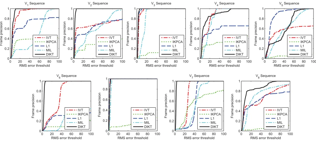
which indicate the ground truth. We also annotate 3–7 fiducial points for the remaining sequences. As usual, our quantitative performance evaluation is based on the root mean square (RMS) errors between the true and the estimated locations of these points [6]. Similar to [45], we additionally present precision plots that visualize the quality of the tracking. Such graphs show the percentage of frames in which the target was tracked with an RMS error less than a certain threshold.
In our experiments, all trackers use an affine motion model with a fixed number of drawn particles (800 particles). In the following, we present the results obtained for two versions of our experimental settings. In the first version, we attempt to optimize the performance of all trackers using video-specific parameters. That is, for each tracker and video, we found the parameters that gave the best performance in terms of robustness (i.e., how many times the tracker went completely off) and accuracy (measured by the RMS error). In the second and most interesting version, we present results by keeping the parameters of each tracker fixed for all videos. Again, we use the parameters that gave the best performance in terms of robustness and accuracy.
1) Tracking With Video-Specific Parameters: We denote by
DIKT-specific, IVT-specific, IKPCA-specific, L1-specific, and MIL-specific the video-specific versions of the trackers. The optimization criterion was the minimization of the RMS error between the true and the estimated location of the points. Apart from the L1-specific tracker (for which the resolution of the template increases geometrically the complexity), the tracking template was chosen to be of resolution of 32×32. For all trackers, we optimized with respect to (wrt) the variance of the Gaussian from which we sample the particles. Expect for the variance of the Gaussian, which is common for all the systems, we optimize.
1) For DIKT-specific, IVT-specific, and IKPCA-specific wrt the number of components (which ranged between 16 and 18) and the variance of the exponential that models the probability of a sample being generated by the learned subspace. For IKPCA-specific we also optimized wrt the radius of the GRBF function. 2) For L1-specific wrt the number of templates and the
res-olution of the template (actually, the tracking becomes impractical when choosing templates of resolution more than 20×20).
3) For MIL-specific wrt the parameters mentioned in [45] (i.e., the number of positives in each frame, the number
TABLE I
MEANRMS ERROR FORVIDEO-SPECIFICTRACKING.
“(LOST)” INDICATESSEQUENCES INWHICH THETRACKER
CLEARLYDOESNOTFOLLOW THETARGETTHROUGHOUT
V1 V2 V3 V4 V5 V6 V7 V8 V9
IVT-specific 6.82 (Lost) 4.07 10.79 (Lost) 3.31 1.78 2.62 (Lost) IKPCA-specific (Lost) (Lost) (Lost) (Lost) (Lost) (Lost) (Lost) (Lost) (Lost) L1-specific 6.17 (Lost) 2.87 11.10 12.68 9.53 1.62 13.58 (Lost) MIL-specific 16.95 (Lost) 13.61 14.62 37.56 12.73 4.14 23.87 17.62 DIKT-specific 4.48 2.27 2.49 5.62 11.28 3.40 1.80 1.96 5.90
TABLE II
MEANRMS ERROR FORGENERALTRACKING. “(LOST)” INDICATES
SEQUENCES INWHICH THETRACKERCLEARLYDOESNOTFOLLOW THE
TARGETTHROUGHOUT
V1 V2 V3 V4 V5 V6 V7 V8 V9
IVT 8.13 (Lost) 4.13 13.14 (Lost) 27.79 2.02 24.48 (Lost)
IKPCA (Lost) (Lost) (Lost) (Lost) (Lost) (Lost) (Lost) (Lost) (Lost)
L1 (Lost) (Lost) 2.87 (Lost) 12.94 (Lost) 1.67 39.15 (Lost)
MIL 51.36 (Lost) 13.61 17.78 38.19 (Lost) 4.14 40.80 (Lost)
DIKT 4.81 2.43 2.49 (Lost) (Lost) 3.51 2.15 2.26 (Lost)
that controls the sampling of negative examples, the learning rate for the weak classifiers, etc).
The tracking rates for the tested systems on a desktop running an Intel Core i7 870 at 2.93 GHz with 8 GB of RAM and MATLAB64 are as follows: for IVT 4 frames/s, for DIKT 3 frames/s, for IKPCA 0.7–1 frame/s, for MIL 0.25 frames/s, and for L1 less than 0.1 frames/s.
For these versions of the trackers, Table I lists the mean RMS error for all sequences, while Fig. 2 plots the RMS error as a function of the frame number. Fig. 3 shows the accuracy in terms of precision plots. Qualitative track-ing results for all methods are shown in Fig. 1. Finally, videos and sample code for DIKT may be found at http:// www.doc.ic.ac.uk/~sl609/dikt/.
In general, DIKT-specific outperforms all other trackers in terms of robustness, accuracy, and precision. In terms of robustness, DIKT-specific successfully follows the target for all sequences, including V2, where all other trackers fail. In
terms of RMS error, DIKT-specific achieves by far the best results for all videos with the exception of video V7, where
it is slightly outperformed by IVT-specific and L1-specific. While MIL-specific appears to be robust (it loses the target for one video sequence only), it is generally not as precise as the other trackers. Clearly, IKPCA is inferior to the other trackers. We believe that this performance degradation is induced by the search for preimages, which accumulates errors and eventually makes the tracker go off in prolonged and challenging video sequences.
2) Tracking With Fixed Parameters: We denote by DIKT,
047
V1
106
V1
107
V1
378
V1
475
V1
573
V1 032
V2
145
V2
259
V2
310
V2
344
V2
478
V2 049
V3
116
V3
166
V3
191
V3
388
V3
461
V3 007
V4
269
V4
499
V4
582
V4
691
V4
746
V4 047
V5
104
V5
128
V5
244
V5
312
V5
464
V5 002
V6
186
V6
227
V6
235
V6
430
V6
657
V6 038
V7
116
V7
231
V7
269
V7
297
V7
393
V7 003
V8
019
V8
164
V8
180
V8
305
V8
473
V8 030
V9
454
V9
612
V9
657
V9
1152
V9
1344
V9 047
V1
106
V1
107
V1
378
V1
475
V1
573
V1 032
V2
145
V2
259
V2
310
V2
344
V2
478
V2 049
V3
116
V3
166
V3
191
V3
388
V3
461
V3 007
V4
269
V4
499
V4
582
V4
691
V4
746
V4 047
V5
104
V5
128
V5
244
V5
312
V5
464
V5 002
V6
186
V6
227
V6
235
V6
430
V6
657
V6 038
V7
116
V7
231
V7
269
V7
297
V7
393
V7 003
V8
019
V8
164
V8
180
V8
305
V8
473
V8 030
V9
454
V9
612
V9
657
V9
1152
V9
1344
[image:8.612.71.540.48.570.2]V9
Fig. 1. Example frames of the tracking with video-specific parameters for V1–V9(top to bottom). The results of DIKT-specific () versus IVT-specific (),
IKPCA-specific (♦), L1-specific (), and MIL-specific () are shown. The ground truth is indicated by×. The tracked area of DIKT-specific is visualized by a magenta bounding box.
set. The number of components for DIKT and IVT was set to 16, and the resolution for all trackers except for L1 was set to 32×32. For all the test videos, we list the mean RMS errors in Table II, while Figs. 4 and 5 illustrate the accuracy and precision of all trackers. The video results can be found at http://www.doc.ic.ac.uk/~sl609/dikt/.
Compared to the performance of all other trackers, that of DIKT appears to be significantly less affected by video-specific parameter fine-tuning. In terms of robustness, DIKT is still among the most robust trackers, because in six out of
nine videos the target was successfully tracked. In terms of accuracy and precision, DIKT appears to be the only tracker that performs almost equally well to its video-specific version (DIKT-specific).
B. Face Recognition
0 100 200 300 400 500 0 50 100 150 Frame RMS error
V1 Sequence
IVT−specific
IKPCA−specific L1−specific MIL−specific DIKT−specific
0 100 200 300 400 500 0 50 100 150 200 250 Frame RMS error
V2 Sequence
IVT−specific
IKPCA−specific L1−specific MIL−specific DIKT−specific
0 100 200 300 400
0 20 40 60 Frame RMS error
V3 Sequence
IVT−specific
IKPCA−specific L1−specific MIL−specific DIKT−specific
0 200 400 600 800
0 20 40 60 80 100 Frame RMS error
V4 Sequence
IVT−specific
IKPCA−specific L1−specific MIL−specific DIKT−specific
0 100 200 300 400 500 0 50 100 150 200 250 Frame RMS error
V5 Sequence
IVT−specific
IKPCA−specific L1−specific MIL−specific DIKT−specific
0 100 200 300 400 500 600 0 20 40 60 Frame RMS error
V6 Sequence
IVT−specific
IKPCA−specific L1−specific MIL−specific DIKT−specific
0 50 100 150 200 250 300 350 0 5 10 15 20 Frame RMS error
V7 Sequence
IVT−specific
IKPCA−specific L1−specific MIL−specific DIKT−specific
0 100 200 300 400 0 20 40 60 80 100 Frame RMS error
V8 Sequence
IVT−specific
IKPCA−specific L1−specific MIL−specific DIKT−specific
0 200 400 600 800 1000 1200 0 50 100 150 Frame RMS error
V9 Sequence
IVT−specific
[image:9.612.50.562.54.353.2]IKPCA−specific L1−specific MIL−specific DIKT−specific
Fig. 2. RMS error for each frame of the tuned DIKT-specific against IVT-specific, IKPCA-specific, L1-specific, and MIL-specific for V1–V9(left to right,
top to bottom). There is no RMS error during complete occlusions.
0 20 40 60 80 100 0 0.2 0.4 0.6 0.8 1
RMS error threshold
Frame precision
V1 Sequence
IVT−specific
IKPCA−specific L1−specific MIL−specific DIKT−specific
0 20 40 60 80 100 0 0.2 0.4 0.6 0.8 1
RMS error threshold
Frame precision
V2 Sequence
IVT−specific
IKPCA−specific L1−specific MIL−specific DIKT−specific
0 20 40 60 80 100 0 0.2 0.4 0.6 0.8 1
RMS error threshold
Frame precision
V3 Sequence
IVT−specific
IKPCA−specific L1−specific MIL−specific DIKT−specific
0 20 40 60 80 100 0 0.2 0.4 0.6 0.8 1
RMS error threshold
Frame precision
V4 Sequence
IVT−specific
IKPCA−specific L1−specific MIL−specific DIKT−specific
0 20 40 60 80 100 0 0.2 0.4 0.6 0.8 1
RMS error threshold
Frame precision
V5 Sequence
IVT−specific
IKPCA−specific L1−specific MIL−specific DIKT−specific
0 20 40 60 80 100 0 0.2 0.4 0.6 0.8 1
RMS error threshold
Frame precision
V6 Sequence
IVT−specific
IKPCA−specific L1−specific MIL−specific DIKT−specific
0 20 40 60 80 100 0 0.2 0.4 0.6 0.8 1
RMS error threshold
Frame precision
V7 Sequence
IVT−specific
IKPCA−specific L1−specific MIL−specific DIKT−specific
0 20 40 60 80 100 0 0.2 0.4 0.6 0.8 1
RMS error threshold
Frame precision
V8 Sequence
IVT−specific
IKPCA−specific L1−specific MIL−specific DIKT−specific
0 20 40 60 80 100 0 0.2 0.4 0.6 0.8 1
RMS error threshold
Frame precision
V9 Sequence
IVT−specific
IKPCA−specific L1−specific MIL−specific DIKT−specific
Fig. 3. Frame precision plots (showing the percentage of frames in which the target was tracked with an RMS error less than a certain threshold) for the tuned DIKT-specific against IVT-specific, IKPCA-specific, L1-specific, and MIL-specific for V1–V9(left to right, top to bottom).
version of our method as seen in Algorithm 1). We compare the results to standard PCA and KPCA with a Gaussian RBF kernel. We optimize the Gaussian RBF kernel’s deviation for each experiment.
1) Extended Yale B Database: The extended Yale B
data-base [48] contains 16 128 images of 38 subjects under 9 poses and 64 illumination conditions. We use a subset
[image:9.612.54.561.398.616.2]0 100 200 300 400 500 0 20 40 60 80 100 Frame RMS error
V1 Sequence
IVT
IKPCA L1 MIL DIKT
0 100 200 300 400 500 0 50 100 150 Frame RMS error
V2 Sequence
IVT
IKPCA L1 MIL DIKT
0 100 200 300 400
0 20 40 60 Frame RMS error
V3 Sequence
IVT
IKPCA L1 MIL DIKT
0 200 400 600 800
0 20 40 60 Frame RMS error
V4 Sequence
IVT
IKPCA L1 MIL DIKT
0 100 200 300 400 500 0 50 100 150 200 250 Frame RMS error
V5 Sequence
IVT
IKPCA L1 MIL DIKT
0 100 200 300 400 500 600 0 50 100 150 200 Frame RMS error
V6 Sequence
IVT
IKPCA L1 MIL DIKT
0 50 100 150 200 250 300 350 0 5 10 15 Frame RMS error
V7 Sequence
IVT
IKPCA L1 MIL DIKT
0 100 200 300 400
0 50 100 150 Frame RMS error
V8 Sequence
IVT
IKPCA L1 MIL DIKT
0 200 400 600 800 1000 1200 0 50 100 150 Frame RMS error
V9 Sequence
IVT
[image:10.612.52.560.52.357.2]IKPCA L1 MIL DIKT
Fig. 4. RMS error for each frame of DIKT against IVT, IKPCA, L1, and MIL for V1−V9(left to right, top to bottom). There is no RMS error during
complete occlusions.
0 20 40 60 80 100 0 0.2 0.4 0.6 0.8 1
RMS error threshold
Frame precision
V1 Sequence
IVT
IKPCA L1 MIL DIKT
0 20 40 60 80 100 0 0.2 0.4 0.6 0.8 1
RMS error threshold
Frame precision
V2 Sequence
IVT
IKPCA L1 MIL DIKT
0 20 40 60 80 100 0 0.2 0.4 0.6 0.8 1
RMS error threshold
Frame precision
V3 Sequence
IVT
IKPCA L1 MIL DIKT
0 20 40 60 80 100 0 0.2 0.4 0.6 0.8 1
RMS error threshold
Frame precision
V4 Sequence
IVT
IKPCA L1 MIL DIKT
0 20 40 60 80 100 0 0.2 0.4 0.6 0.8 1
RMS error threshold
Frame precision
V5 Sequence
IVT
IKPCA L1 MIL DIKT
0 20 40 60 80 100 0 0.2 0.4 0.6 0.8 1
RMS error threshold
Frame precision
V6 Sequence
IVT
IKPCA L1 MIL DIKT
0 20 40 60 80 100 0 0.2 0.4 0.6 0.8 1
RMS error threshold
Frame precision IVT IKPCA L1 MIL DIKT
0 20 40 60 80 100 0 0.2 0.4 0.6 0.8 1
RMS error threshold
Frame precision
V7 Sequence
IVT
IKPCA L1 MIL DIKT
0 20 40 60 80 100 0 0.2 0.4 0.6 0.8 1
RMS error threshold
Frame precision
V8 Sequence
IVT
IKPCA L1 MIL DIKT
Fig. 5. Frame precision plots (showing the percentage of frames in which the target was tracked with an RMS error less than a certain threshold) for DIKT against IVT, IKPCA, L1, and MIL for V1–V9(left to right, top to bottom).
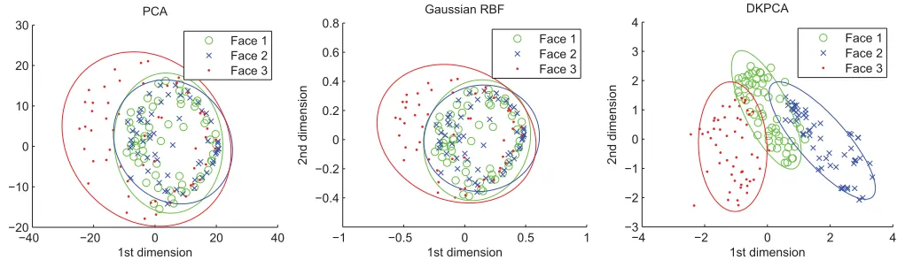
Furthermore, we train each method with the same random selection of three classes, each class with the same five random training images. After computing the subspace of each algo-rithm (linear PCA, KPCA with Gaussian RBF kernel, and the proposed DKPCA), we project the samples of the test set onto it (the deviation of the RBF kernel was set to the one that gave
[image:10.612.53.559.395.621.2]−40 −20 0 20 40 −20
−10 0 10 20 30
1st dimension
2nd dimension
PCA
Face 1 Face 2 Face 3
−1 −0.5 0 0.5 1
−0.4 −0.2 0 0.2 0.4 0.6 0.8
1st dimension
2nd dimension
Gaussian RBF
Face 1 Face 2 Face 3
−4 −2 0 2 4
−3 −2 −1 0 1 2 3 4
1st dimension
2nd dimension
DKPCA
[image:11.612.56.562.53.200.2]Face 1 Face 2 Face 3
Fig. 6. Test data, as projected by the learned subspaces of PCA, Gaussian RBF, and DKPCA (left to right). We train with three randomly selected classes (i.e., subjects) in the usual manner (trained on five). We then plot the corresponding projections of the test samples.
TABLE III
AVERAGERECOGNITIONRATEWITHYALEDATABASE
Trained on 5 Trained on 10 Trained on 20
PCA 31.1% 45.2% 59.3%
Gaussian RBF 31.6% 45.5% 59.4%
DKPCA 62.1% 77.7% 88.4%
TABLE IV
AVERAGERECOGNITIONRATEWITHCMU PIE DATABASE
Trained on 5 Trained on 10
PCA 26.1% 39.1%
Gaussian RBF 26.1% 39.1%
DKPCA 52.3% 69.4%
The enhanced class-separability achieved by the proposed method can be explained by the metric multidimensional scaling (MMS) perspective of PCA, which can be pro-vided through [49] and [50]. Under this perspective, stan-dard 2 PCA finds the optimal linear projections that best
preserve the 2 distances. As is well known, these
dis-tances can be arbitrarily biased by the presence of outliers (the same holds for KPCA with Gaussian RBF kernels). Therefore, in the presence of outliers, PCA and KPCA with Gaussian RBF are not suitable for providing a consistent way of measuring distances in a facial class. On the other hand, under the MMS perspective, the proposed DKPCA finds the optimal linear projections that best preserve the proposed robust distance. And because, as we argue in our paper, this distance is robust to outliers, the proposed DKPCA provides a more consistent way of representing the samples in a facial class.
2) CMU PIE Database: Our final tests are conducted
with the CMU PIE database [51]. The dataset consists of more than 41 000 face images of 68 subjects. The data-base contains faces under varying pose, illumination, and expression. We use the near frontal poses (C05, C07, C09, C27, and C29) and a total of 170 images for each sub-ject. For training, we randomly selected a subset with 5 or 10 images per subject. For testing, we utilize the remaining images. Finally, we perform 20 different random
realizations of the training and test sets. The results are shown in Table IV.
VI. CONCLUSION
We proposed a robust online kernel learning framework for efficient visual tracking. We used a nonlinear appearance model learned via KPCA and a robust gradient-based kernel. As this kernel is not semipositive definite, we showed how to extend the KPCA formulation into Krein spaces. Finally, we showed that our kernel has a very special form which enables us to formulate a direct version of KPCA in Krein space and does not require the calculation of preimages. Based on this property, we then proposed an efficient and exact incremental KPCA. By combining our appearance model with a particle filter, the proposed tracking framework achieved state-of-the-art performance in many popular difficult tracking scenarios. We showed further applications of our kernel framework by testing on face recognition, for which we improve upon 2-norm PCA and KPCA in Hilbert space with a Gaussian
RBF kernel.
In future work, we intend to apply our kernel framework to other applications which would benefit from its robustness. In relation to tracking, we plan to investigate the influence of the forgetting factor to our incremental KPCA in Krein space.
APPENDIX
KERNELPROPERTIES
Let kernel k :Cd ×Cd → R be the kernel from (7) and
xi,xj ∈Cd are two samples.
Lemma 1: dc=1R(c)≤
√
ddc=1R2(c).
Proof: We show for any d-dimensional R∈R+
d
c=1
R(c)≤√d
d
c=1 R2(c)
⇔ d
c=1 R(c)
d
c=1
R(c)≤d d
c=1 R2(c)
⇔ d
c=1
R2(c)+2
d−1
c=1 d
e=c+1