University of Warwick institutional repository: http://go.warwick.ac.uk/wrap
This paper is made available online in accordance with publisher policies. Please scroll down to view the document itself. Please refer to the repository record for this item and our policy information available from the repository home page for further information.
To see the final version of this paper please visit the publisher’s website. Access to the published version may require a subscription.
Author(s): Kefeng Zhang, Duncan J. Greenwood, William P.
Spracklen, Clive R. Rahn, John P. Hammond, Philip J. White and Ian G. Burns
Article Title: A universal agro-hydrological model for water and nitrogen cycles in the soil–crop system SMCR_N: Critical update and further validation
Year of publication: 2010 Link to published version:
1
A universal agro-hydrological model for water and nitrogen cycles in the soil-2
crop system SMCR_N: critical update and further validation 3
4
Kefeng Zhang1,3, Duncan J Greenwood1, William P Spracklen1, Clive R Rahn1, John 5
P Hammond1, Philip J White2, Ian G Burns1 6
7
1
Warwick-HRI, Warwick University, Wellesbourne, Warwick, CV35 9EF, UK. 8
2
Scottish Crop Research Institute, Invergowrie, Dundee, DD2 5DA, UK 9
3
Corresponding author 10
11
Corresponding author: Kefeng Zhang 12
Address: Warwick-HRI, The University of Warwick, 13
Wellesbourne, Warwick, CV35 9EF, UK 14
Tel: 0044 24 7657 4996
15
Fax: 0044 24 7657 4500
16
Email: [email protected]; [email protected] (K. Zhang) 17
18
Running title: A universal model for crop water and N cycles 19
20
Number of text pages: 28 21
Number of tables: 5 22
Number of figures: 11 23
Abstract 1
2
Agro-hydrological models have widely been used for optimising resources use and 3
minimizing environmental consequences in agriculture. SMCR_N is a recently 4
developed sophisticated model which simulates crop response to nitrogen fertilizer for 5
a wide range of crops, and the associated leaching of nitrate from arable soils. In this 6
paper, we describe the improvements of this model by replacing the existing 7
approximate hydrological cascade algorithm with a new simple and explicit algorithm 8
for the basic soil water flow equation, which not only enhanced the model 9
performance in hydrological simulation, but also was essential to extend the model 10
application to the situations where the capillary flow is important. As a result, the 11
updated SMCR_N model could be used for more accurate study of water dynamics in 12
the soil-crop system. The success of the model update was demonstrated by the 13
simulated results that the updated model consistently out-performed the original 14
model in drainage simulations and in predicting time course soil water content in 15
different layers in the soil-wheat system. Tests of the updated SMCR_N model 16
against data from 4 field crop experiments showed that crop nitrogen offtakes and soil 17
mineral nitrogen in the top 90 cm were in a good agreement with the measured values, 18
indicating that the model could make more reliable predictions of nitrogen fate in the 19
crop-soil system, and thus provides a useful platform to assess the impacts of nitrogen 20
fertilizer on crop yield and nitrogen leaching from different production systems. 21
22
Key words: soil-crop system, modeling, water and nitrogen transfer, agricultural 23
water management, nitrogen management, nitrogen leaching. 24
1. Introduction 1
2
Agro-hydrological models have proved to be useful tools in optimizing 3
irrigation scheduling and fertilizer application, and in assessing the impact of different 4
farming practices on the environment. Numerous models for various crop species 5
have been reported for these purposes in the literature in the last few decades 6
(Johnsson et al., 1987; Bergstrom et al., 1991; Williams et al., 1993; Diekkruger et al., 7
1995; Hoogenboom et al., 1999; Brisson et al., 2003; Jones et al., 2003; Keating et al., 8
2003; Stöckle et al., 2003; van Ittersum et al., 2003; Zhang et al., 2007, 2009; Rahn et 9
al., 2010). 10
11
A large number of agro-hydrological models are devoted to assessing the 12
effects of nitrogen (N) fertilizer on crop growth and N leaching for various crop 13
species (see the review by Cannavo et al., 2008). The most prominent models that 14
cover a range of crops are the EPIC models (Williams et al., 1993) and the DSSAT 15
models (Hoogenboom et al., 1999). Although the EPIC and DSSAT models have 16
proved useful in both basic and applied studies of the effects of climate and 17
management on growth and the environment, the models are generally crop specific, 18
and require parameter values which are difficult to determine for a given crop. Lack 19
of generality is a common feature for crop N models. According to the recent review 20
by Cannavo et al. (2008) where 62 crop N models were surveyed, only 2 models are 21
able to simulate the N cycle for 4 crops families, while a vast majority of the models 22
are only able to deal with a single crop, mainly cereal crops. This has caused 23
difficulties in the use of models for optimizing N inputs in crop production where 24
effects of N fertilizer on crop growth and the associated N leaching is evidently 1
important. 2
3
A new crop N model named SMCR_N model, which is based on a version of 4
N_ABLE (Greenwood, 2001) and EU-Rotate_N (Rahn et al., 2010), has been 5
developed for crop N response and N leaching in arable soils (Zhang et al., 2009). 6
The model covers a wide range of crops, which makes it a good candidate for 7
forecasting both optimum N inputs and the environmental consequences of crop 8
production. Compared with most models of its kind, the SMCR_N model is much 9
more mechanistically based. A promising degree of agreement was found between 10
predictions of the SMCR_N model and actual measurements of responses of crop 11
yield and N mineral composition to N fertilizer from 32 field experiments over 16 12
crops (Zhang et al., 2009). However, the model at present uses an approximate 13
cascade type of algorithm to calculate the redistribution of water and nitrate and losses 14
by percolation and leaching from the soil profile. Although this approach is simple 15
and easy to implement, it is unable to simulate capillary flow and can give poor 16
predictions of daily soil water changes (Gandolfi et al., 2006; Cannavo et al., 2008; 17
Yang et al., 2009). It is therefore unsatisfactory for some circumstances including 18
those where the groundwater table is high and thus upward capillary flow can largely 19
satisfy demands of evapotranspiration (Yang et al., 2009). Moreover, it is difficult to 20
implement boundary conditions precisely at the lower boundary in the cascade model, 21
which could result in unreliable predictions as the hydrological simulations are highly 22
sensitive to the parameterization at the lower boundary (Boone and Wetzel, 1996). 23
It is well known that a numerical approach using the Richards’ equation could 1
simulate soil water movement more accurately. Such a basic theory of water 2
movement in soil is now widely accepted but, despite substantial advances in 3
mathematics and computer science, the uptake of models of this type is still low 4
(Bastiaanssen et al. 2007). One reason for this is the complex nature of the numerical 5
methods involved, and the resulting long program code. In spite of the fact that the 6
numerical schemes such as the finite element (FE) method for solution to the 7
Richards’ equation are well developed (Šimunek et al., 1992), their use requires 8
specialized expertise that many potential users have not got. This has led to the 9
adoption of cascade method for soil water movement in many agro-hydrological 10
models on fertilizer, irrigation and pesticide practices. For example, Cannavo et al. 11
(2008) found that a large proportion of crop N models (7 out of 16) adapted the 12
cascade approach for hydrological simulations, while Ranatunga et al. (2008) reported 13
that the majority of soil water models (13 out of 21) that have been widely applied in 14
Australia using a similar method. In order to address this problem, a promising 15
alternative algorithm, based on the work by Lee and Abriola (1999), has been 16
proposed to simulate water dynamics in the soil-crop system where the Richards’ 17
equation was employed for the description of soil water movement (Yang et al., 2009). 18
The algorithm considers that the water content in a soil layer in a small time step of 19
0.001 d is only influenced by its adjacent layers, i.e. those immediately above and 20
below. It has been demonstrated that the simple and explicit algorithm could 21
accurately reproduce the spatial-temporal soil water content in the cropped soils 22
(Yang et al., 2009). 23
The primary objectives of the study include: 1) update the SMCR_N model 1
(Zhang et al., 2009) with the recently developed simple and highly accurate algorithm 2
(Yang et al., 2009) for hydrological simulations; 2) to compare the simulated values 3
of soil water distribution made by the updated model, the original model, and the 4
highly accurate FE procedure in modeling water drainage in contrasting soils; 3) to 5
compare the performance of the updated SMCR_N model with the original version in 6
predicting soil water dynamics in the soil-wheat system; 4) to validate the updated 7
SMCR_N model against data of crop N and soil mineral-N from new field 8
experiments on 4 different crops. 9
10
2. The model 11
12
2.1. Model framework 13
14
The SMCR_N model (Zhang et al., 2009) operates on uniform 5 cm soil layers 15
that are widely used in the agro-hydrological models to describe processes such as 16
root length distribution in the soil-crop system (Greenwood, 2001, Zhang et al., 2007, 17
Renaud et al., 2008, Yang et al., 2009; Pedersen et al., 2010; Rahn et al., 2010). It is 18
not our intention to present a detailed description of the whole model here since the 19
SMCR_N model has been published (Zhang et al., 2009). Instead we focus on the 20
modifications to the model, i.e. the new hydrology module, and its performance in 21
simulating soil water drainage and soil water dynamics in the soil-crop system. We 22
also focus on the validation of the updated model against data from new field 23
experiments. However, to help to understand the model framework, we provide the 24
of the principles and the key equations included in the other major modules. The 1
justification of employing the equations in these modules can be seen in Zhang et al. 2
(2009). 3
4
The updated model differs from its predecessor in that two time steps are 5
employed. The model calculates plant dry matter accumulation, root length 6
distribution, potential evaporation, and potential N and water requirements for plant 7
growth on a daily basis, whereas a much smaller time step of 0.001 d is implemented 8
in the algorithms for calculating actual soil evaporation, water and N uptake by roots, 9
and soil water and N movement. The implementation of such procedures is similar 10
with that for modeling water transfer in the soil-crop system (Yang et al., 2009). 11
12
2.2 Hydrology module 13
14
In a 1-D situation, the Richards’ equation governing water flow under gravity 15
in an isotropic variably saturated soil is (Celia et al. 1990; Šimunek et al., 1992; 16
Zhang et al., 2010): 17
18
)] 1 )( ( [
z h K z
t (1)
19
20
where (cm3 cm-3) is the volumetric soil water content, t (d) is time, K (cm d-1) is the 21
soil hydraulic conductivity, h (cm) is the soil pressure head, and z (cm) is the vertical 22
coordinate. 23
The soil hydraulic functions are defined according to van Genuchten (1980) 1
and Mualem (1976): 2 3 m n r s r
h| ]
| 1
1
[ (2)
4 5 2 / 1 5 . 0 ] ) 1 ( 1 [ )
( m m
s K
K (3)
6
7
where is the relative saturation, s and r (cm 3
cm-3) are the saturated and residual 8
soil water contents, (cm-1) and n are the shape parameters of the retention and 9
conductivity functions, m=1-1/n, and Ks (cm d-1) is the saturated hydraulic
10
conductivity. 11
12
Integrating Eq. (1) vertically over a soil layer leads to (Lee and Abriola, 1999; 13
Yang et al., 2009): 14 15 ) ( 1 1 i i i w w z
t (4)
16 17 where 18 19 ) 1 ( 1 z h h K
wi i i i (5)
20
21
in which i is the soil layer number, numbered from 1 at the bottom layer of the profile 22
soil layer thickness, wi+1,wi (cm d-1) are the water fluxes from layer i+1 to i, and i to
i-1
1, respectively, i (cm3 cm-3) is the layer-average soil water content change in layer 2
i in t, and hi and hi 1 (cm) are the soil pressure head in the layers i and i-1, 3
respectively. 4
5
When rainfall plus irrigation are greater than the potential evaporation, the 6
water flux from the surface is considered as infiltration. The actual infiltration flux, 7
act
I (cm d-1), is determined by the following equation (Yang et al., 2009): 8
9
]} , / ) min[(
,
min{K z t R
Iact s s Top (6)
10
11
in which R (cm d-1) is the possible net water flux at the surface, and Top is the water
12
content in the top soil layer. 13
14
If the potential evaporation exceeds the sum of rainfall and irrigation, the 15
actual evaporation in a given time step from the top soil layer, Eact (cm d-1), is 16
expressed as (Yang et al., 2009): 17
18
} ], 1 / ) [(
min{K hm in h z R
Eact Top Top (7)
19
20
where KTop (cm d-1) and hTop (cm) are the hydraulic conductivity and soil pressure
21
head in the top layer, respectively, and hmin (cm) is the minimum soil pressure head
22
head corresponding to half water content at the permanent wilting point as 1
recommended by the FAO (Allen et al., 1998). 2
3
The treatment of N transport in the soil is simple. The proportion of N 4
transported from a soil layer is considered to be identical to the ratio of water drainage 5
out of the layer to the total water in the layer (Burns, 1974; Greenwood, 2001; Zhang 6
et al., 2007, 2009; Pedersen et al., 2010). Diffusion terms for N transport in the soil 7
are not included in the simulation. 8
9
2.3 Plant growth module 10
11
The actual daily increments in plant dry weight excluding the fibrous roots are 12
calculated by a growth equation which allows the crop to grow exponentially in the 13
early growth stages and linearly towards maturity (Greenwood, 2001; Zhang et al., 14
2007, 2009). 15
16
W K
W K W
1 2
) 1 , %
% min(
crit N
N
(8) 17
18
where ∆W (t ha-1
) is the maximum possible increment in growth on the day, W (t ha-1) 19
is the dry weight of the entire plant excluding fibrous roots, K1 (=1 t ha-1) is the
semi-20
maximum W for growth rate, K2 (t ha-1 d-1) is a growth rate coefficient, which can be
21
calculated using the specified target yield, the dry weight at planting and daily mean 22
air temperature (Zhang et al., 2009), %N is the percentage of N in W, %Ncrit is the
23
critical %N, i.e. the minimum %N at which growth proceeds at the maximum rate, 24
1
) 1
(
%Ncrit N Ne 0.26W (9)
2
3
where and βN are crop specific parameters that relate critical %N to crop dry
4
weight. 5
6
In the case of crop capable of luxury N consumption, the possible maximum 7
crop %N in the plant is calculated as follows: 8 9 crit lux N R N %
% m ax (10)
10
11
where Rlux is the coefficient of crop luxury N consumption.
12
13
The increment in root dry weight Wr is considered as a function of the 14
increment in crop dry weight W , crop dry weight W, and a parameter defining root 15
class (Zhang et al., 2009; Pedersen et al., 2010). The total root length is calculated 16
from a fixed specific root length and root dry weight Wr. The root penetration down
17
the soil profile is driven by the accumulative daily mean air temperature. The root 18
length declines logarithmically from the soil surface downwards (Pedersen et al., 19 2010). 20 21 } , ] ) ( , 0 max[
min{ z0 lag rz zmax
z R T T K R
1
where Rz (m) is the simulated rooting depth, Rz0 (m) is the starting rooting depth,
2
T (oC d) is the cumulative day degree, Tlag (oC d) is the threshold of cumulative
3
day degree for root growth, Krz (m day-1 C-1) is the root growth rate, Rzmax (m) is the
4
maximum rooting depth restricted by physical barriers, L0 (m m-3) is the total root
5
length, and az is the shape parameter controlling root distribution down the profile.
6
More information about modeling root development is given elsewhere (Pedersen et 7
al., 2010). 8
9
2.4 N and water requirements module 10
11
Crops are considered to have two N compartments: a top N compartment and a 12
root N compartment (Zhang et al., 2009). The top N compartment contains N of the 13
entire plant excluding N in fibrous roots, whereas the root N compartment stores N 14
allocated in fibrous roots. The demands of N in the top and root compartments are 15
calculated as (Zhang et al., 2009): 16
17
] % %
) [(
10 W W Nm ax W N
UN (13)
18
] % %
) [(
10 r r rpot r r
Nr W W N W N
U (14)
19
20
where UN and UNr (kg N ha-1) are the potential N uptake in the top and root
21
compartments, respectively, %Nr is the actual %N in Wr, and %Nrpot is the root
22
potential %N, which is calculated from (Zhang et al., 2009): 23
24
W N
rpot e
N 1 0.26
% (15)
1
The potential soil evaporation and plant transpiration are calculated according 2
to the FAO 56 crop coefficient method (Allen et al., 1998): 3
4
0 ET K
Epot e (16)
5
0 ET K
Tpot cb (17)
6
7
where Epot and Tpot are the potential soil evaporation and plant transpiration,
8
respectively, Ke is the evaporation coefficient, Kcb, dependent on crop species and its
9
development stage, is the basal crop coefficient for transpiration, ET0 (mm) is the
10
reference evapotranspiration. ET0, Kcb, Kcmax and f can be determined according to
11
Allen et al. (1998). 12
13
2.5 N and water uptake module 14
15
N uptake is calculated according to crop N demand, root length distribution, 16
soil mineral N concentration and the minimum soil mineral N concentration for root 17
uptake, as proposed by Pedersen et al. (2010). 18
19
) 1
)(
( N Nr
pot U U N Nr N
act U U e
N (18) 20 21 in which 22 23 0 m in) ( ) ( c c c c k z L N N N N N
pot (19)
1
where Nact (kg N ha-1) and Npot (kg N ha-1) are the actual and potential N uptake,
2
respectively, cN (kg N m-3) is the soil mineral N concentration in soil layer, cNmin (kg
3
N m-3) is the minimum soil mineral N concentration, c0 (kg N m-3) is the plant N
4
uptake coefficient, and kN is the plant N uptake efficiency (Pedersen et al., 2010).
5
6
The actual crop transpirationTact (cm d-1) is the sum of root water uptake from 7
different layers. It is formulated (Zhang et al., 2009, 2010), 8
9
act
T w(h)L(z)Tpot/ L(z) (20)
10 11 in which 12 13 1 2 2 3 3 2 3 1 3 1 ) /( ) ( , 0 ) ( h h h h h h h h h h h h h h h w (21) 14 15
where w is the root water stress reduction factor. Root water uptake is assumed to be
16
zero when soil pressure head is below h3, i.e. the soil pressure head at the permanent
17
wilting point (h3 = -15000 cm), and is unlimited for soil pressure head between h1 (-1
18
cm) and h2high (-500 cm) for a rapid transpiration (0.5 cm d -1
) and h2low (-1100 cm) for
19
a slow transpiration (0.1 cm d-1). The increase in water uptake between h3 and h2 is
20
linearly related to the soil pressure head. Water uptake is also assumed to be 0 for soil 21
pressure head greater h1 due to lack of oxygen in the root zone (Zhang et al., 2009,
22
1
2.6 N mineralization module 2
3
N mineralization from soil organic matter is considered in the model. The 4
algorithm is devised based on the assumption that the organic matter breakdown rate 5
is a first-order process. Daily N mineralization from soil organic matter is estimated 6
as follows (Zhang et al., 2009). 7
8
5 min
10 10 min
min 10
CN c s s T T
s
R m Z Q
k N
s
(22)
9
10
where Nsmin (kg ha-1) is the daily N mineralization rate from soil organic matter, kmin
11
(d-1) is the temperature-independent coefficient for the rate of organic matter 12
oxidation, 10 10
s T T
Q is the correction factor of temperature on N mineralization, s (g
13
cm-3) is the soil bulk density, Zsmin (cm) is the soil depth where N mineralization takes
14
place, mC (%) is the soil organic C content, RCN is the C:N ratio of the soil organic
15
matter, Ts (oC) is the base temperature at which 1010 s T T
Q equals 1, and Q10 is the factor
16
change in rate with a 10 degree change in temperature. 17
18
3. Experiments 19
20
Experiments on two sites are described in this section. The results of an 21
experiment (PAGV experiment) carried out at the Institute for Soil Fertility Research, 22
Netherlands (Groot and Verberne, 1991) are used to compare the updated and the 23
system, while the experiments (HRI experiments) conducted at Warwick-HRI, 1
Warwick University, UK are used for the validation of the updated model. 2
3
3.1 PAGV experiment for model comparison 4
5
The experiment used in model comparison between the updated and the 6
original versions was conducted in the PAGV farm with winter wheat at the Institute 7
for Soil Fertility Research, Netherlands in 1984 (Groot and Verberne, 1991). The crop 8
was sown on 21 October, 1983 and harvested on 21 August, 1984. The soil in the 9
PAGV farm was silty loam. The measurements of soil water in the layers of 0-20, 20-10
40, 40-60, 60-80 and 80-100 cm were made at intervals of three weeks from 14 11
February, 1984. Also the time-course of groundwater tables were measured. Detailed 12
description of the experiment and measured weather and soil water data can be seen in 13
Groot and Verberne (1991). 14
15
3.2 HRI experiments for model validation 16
17
To validate the updated model, field experiments with four contrasting crops 18
were carried out using a completely randomized design on a sandy loam soil at 19
Wellesbourne, Warwick-HRI, UK in 2006. The crops were radish (grown over a very 20
short period and had a small yield), lettuce and cabbage (grown over longer periods 21
and had reasonable yields), and soyabean (a legume and able to fix atmospheric-N). 22
Radish and soyabean were drilled directly, whereas lettuce and cabbage were 23
transplanted using plants raised separately in peat blocks. The experimental plots were 24
soyabean. For each crop plants were grown in 3 different plots. N fertiliser was 1
broadcast (as NH4NO3) at a rate of 100 kg N ha-1 on all plots and incorporated to a
2
depth of 10 cm before drilling or transplanting; a further 200 kg N ha-1 was top 3
dressed for cabbage at a later date. Applications of other major nutrients, and weed 4
and pest control measures followed normal practice. Further cropping data and other 5
details of the experiments are summarised in Table 1. Three replicate plants from each 6
plot of each crop were randomly selected and harvested at maturity in the end of the 7
experiments. Sub-samples were dried at 80oC to constant weight and then analysed 8
for %N (CN-2000, LECO). 9
10
Pre-planting soil samples were taken for mineral N to a 30 cm depth on 5 11
December 2005 for lettuce and radish, and on 6 February 2006 for cabbage and 12
soyabean, respectively. After harvesting, further soil samples were taken to 90 cm 13
depth on 31 January 2007 for cabbage, 7 February 2007 for soyabean, and 19 14
February 2007 for lettuce and radish, respectively. 15
16
4. Model parameterization 17
18
The study was carried out in two parts. In the first part, the performance of the 19
updated model against the original model in hydrological simulations was carried out. 20
This was done by running the models for water drainage in contrasting soils via a 21
numerical experiment, and for soil water dynamics in the PAGV experiment. The 22
results were compared against these from an alternative method and the measurements. 23
The second part involved comparing the predictions of the updated SMCR_N model 24
1
4.1 Numerical and PAGV experiments for model comparison 2
3
4.1.1 Numerical experiment 4
5
To examine how the new hydrology module performed in simulating water 6
drainage in soil columns, it was compared with two alternative methods, i.e. the 7
cascade method originally employed in the SMCR_N model and the highly accurate 8
FE method for solving the soil water flow equation. The simulations were carried out 9
on two contrasting soils: a very coarse soil and a very fine soil. The parameters 10
describing water characteristics for both soils were set to those suggested by Wösten 11
et al. (1999) (see Table 2 for details). The soil columns were assumed to have a depth 12
of 2 m, with an initial soil water content set at saturation throughout the column. The 13
lower boundary condition was specified as free drainage, whereas no water flux was 14
allowed at the surface. In the updated model, the soil column was divided into 40 15
uniform 5 cm layers, with a simulation time step for both soils of 0.001 d, similar to 16
that proposed by Lee and Abriola (1999) and Yang et al. (2009). In the FE model 17
(Šimunek et al., 1992), the soil domain was divided into 50 soil layers with various 18
thicknesses (thin layers at the bottom where the lower boundary condition was 19
imposed). In the cascade algorithm in the original SMCR_N model, the division of 20
soil column was the same as that in the updated model, i.e. 5 cm each. Drainage 21
occurred only when soil water content exceeded its field capacity. The drainage 22
coefficient was calculated as the ratio of the difference between volumetric soil water 23
contents at saturation and field capacity, to the soil water content at saturation, and the 24
1
4.1.2 PAGV experiment 2
3
Soil water retention curves for the PAGV experiment (0-25, 25-40 and 40-100 4
cm) were measured (Groot and Verberne, 1991). The van Genuchten soil hydraulic 5
property parameters (Eqs. (2)(3)) were fitted (Table 3) using the RETC software (van 6
Genuchten et al., 1991), based on the measured data. The soil hydraulic properties 7
below 100 cm were taken to be the same as those in the layer immediately above. 8
Since the groundwater table in the experiment was frequently measured and ranged 9
from 86 to 173 cm below the surface, the simulated soil depth was considered to be 10
the distance from the surface to the groundwater table and the soil water content at the 11
lower boundary was set at saturation (Yang et al., 2009). 12
13
The crop parameters concerning root growth and root length distribution down 14
the profile were set as follows (see Yang et al., 2009): the root penetration rate Krz of
15
0.0007 m d-1 oC-1, the shape parameter controlling root distribution az of 3.0, the
16
threshold day temperature for root growth Tbase of 7 oC, the temperature for the
17
maximum root growth Trmax of 27 oC. The parameter values used for estimating
18
potential soil evaporation and crop transpiration were according to the FAO dual crop 19
coefficient approach proposed by Allen et al. (1998). The small time step for 20
calculating evaporation, root water uptake and soil water redistribution was 0.001 d 21
(Yang et al., 2009). The weather information used in the simulation periods, including 22
daily air temperatures, rainfall and global radiation, was measured and given in Groot 23
starting point in the simulations and set the measured soil water distributions down 1
the profile as the initial conditions. 2
3
4.2 HRI experiments for the validation of the updated model 4
5
The second part of the study compares the predictions of the updated 6
SMCR_N model against data from the field experiments. Daily measurements of 7
weather variables were made at the on-site weather station. Soil hydraulic properties 8
at various depths are shown in Table 4 (after Fernández-Gálves and Simmonds, 2006). 9
Table 5 lists the parameter values related to crop N-nutritional characteristics, root 10
development, and staged potential evapotranspiration of 4 different species. Such a 11
parameterization over a wide range of crops is given in Zhang et al. (2009). The 12
measured soil mineral N in the top 30 cm was 28.5 kg N ha-1 for lettuce, 10.3 kg N ha -13
1
for radish, and 17.8 kg N ha-1 for cabbage and soyabean. Soil mineral N in 30-60 cm 14
layer and 60-90 cm were estimated as 10 and 5 kg N ha-1, respectively (Zhang et al., 15
2007). The model was run from 5 December 2005 when the pre-planting soil 16
sampling was carried out for lettuce and radish. At this time, the initial soil water 17
deficit then was assumed to be zero, i.e the soil water content in the profile was at 18
field capacity. The simulated amounts of soil mineral N were updated for cabbage and 19
soyabean on 6 February 2006 when soil mineral N was measured on these plots. The 20
minimum soil mineral N level cNmin below which plants are not able to take up N was
21
set 0.0035 kg m-3 for all crops (Zhang et al., 2009). Soyabean was different from other 22
crops in that it fixed atmospheric-N to meet crop critical %N form maximum growth 23
when N supply from the soil was limited. The temperature-independent organic 24
matter breakdown rate kmin was 0.00015 g g-1 d-1 (Zhang et al., 2009), in agreement
with that used in other models for similar soils (Mueller et al., 1996; Fang et al., 2005). 1
The measured organic carbon contents were 0.8% for lettuce, 0.5% for cabbage, 0.6% 2
for radish and 0.9% for soyabean, respectively. The variation in organic carbon 3
content might be due to the incorporation of different previous crop residues and roots. 4
A value of 3 was used for Q10, a factor for correcting rates of organic matter
5
breakdown for differences in temperature (Hansen et al., 1990). The temperature at 6
which the response function for soil temperature on N mineralization equals 1 was set 7
20 oC (Hansen et al., 1990). It was also assumed that soil N mineralization was 8
restricted to the upper 30cm depth of soil. 9
10
5. Results and discussion 11
12
5.1. Numerical experiment 13
14
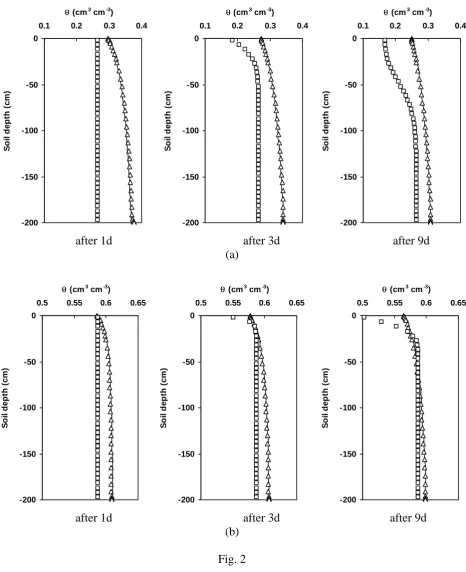
Fig. 2 compares the soil water content profiles at various time intervals 15
simulated with different approaches. The profiles predicted by the updated SMCR_N 16
model agree well with those from the Richards’ equation solved with the FE method. 17
Over the simulation period of 30 days, the maximum error of the proposed approach 18
did not exceed 1% for the coarse soil compared to the FE solution, whereas the 19
maximum error for the fine soil did not exceed 0.8%. However, soil water profiles 20
simulated using the cascade approach in the original SMCR_N model were markedly 21
different from those obtained by the FE method throughout both the soil profile and 22
the simulation period. This is particularly true for the coarse soil (Fig. 2a). The 23
maximum error occurred deeper in the soil column at the early stages of simulation, 24
profile computed by the cascade model under-predicted the soil water content at the 1
bottom of the column compared to the FE solution by 28.7% for the coarse soil and by 2
3.5% for the fine soil. At t = 3 and 9 d, the maximum error increased to 32.3% and 3
33.6% for the coarse soil, respectively. Likewise, the relative differences were 4.7% 4
and 11% for the fine soil. All of the maximum errors moved up to the surface of the 5
soil columns over time. Since soil water content in the near-surface regions of soil are 6
an important determinant of moisture and energy fluxes to the atmosphere (Shao and 7
Henderson-Sellers, 1996; Lee and Abriola, 1999), incorrect simulation of soil water 8
content in this region inevitably affects the estimates of evaporation and vegetation 9
transpiration. 10
11
Fig. 3 compares the total water in the soil column during the simulation period 12
by the different approaches. Again the simulated results from the updated model are 13
in excellent agreement with those from the FE method. In both cases, the maximum 14
error in the whole simulation period was no greater than 1%. In contrast, the results 15
from the cascade model deviated from the FE solution significantly, especially for the 16
coarse soil. At t = 24 h, the cascade model over-predicted drainage from the soil 17
column by 23.3% for the coarse soil, compared with the FE solution. The relative 18
error for the rest of simulation period ranged from 16% to 29%. For the fine soil, the 19
performance of the cascade model was satisfactory in predicting drainage, with the 20
maximum relative error all within 3%. This can be attributed to the slow water flow in 21
this soil. The computed water fluxes at the lower boundary are similar for all the 22
methods, but the distributions of water contents are noticeably different in the near-23
surface region (Fig. 2). 24
5.2. PGAV experiment 1
2
To evaluate the overall model performance in predicting soil water dynamics 3
in the soil-crop system where all the processes governing water transfer from soil to 4
the atmosphere were considered, all the measurements of soil water content from the 5
experiment in different soil layers at time intervals were compared with the 6
simulations by the updated and the original models (Fig. 4). Regressions of simulated 7
and measured gave a similar R2 value for both models, which suggests that both the 8
original and the updated models were all able to simulate the change patterns in soil 9
water content. However, the gradient of approximately to 1 and the intercept of 10
approximately to 0.0 from the updated model show that the simulated values of soil 11
water content from the updated model agreed much better with the measured values 12
(all the data points are close to the 1:1 line) than those from the original model. 13
14
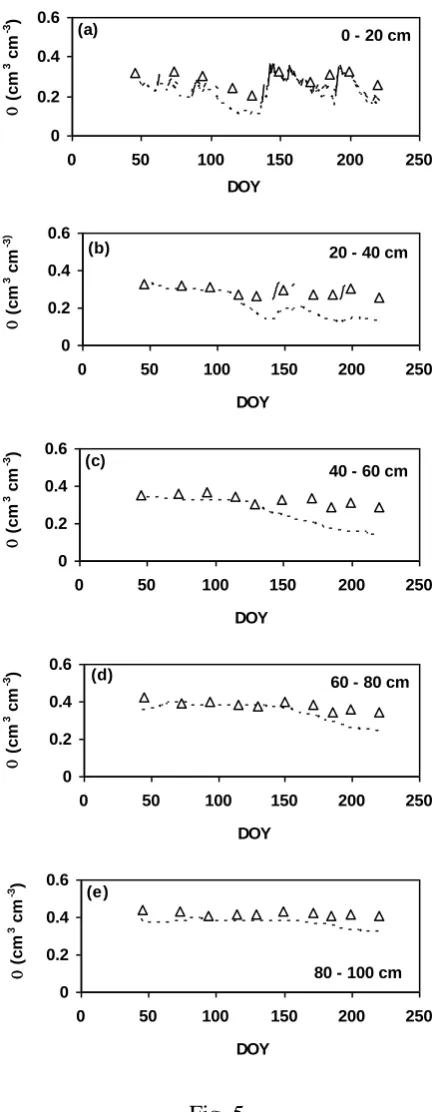
Soil water contents in 20 cm layers to 1 m were compared between the 15
measured and the simulated using the updated and the original models in detail over 16
time (Fig. 5). It can be observed that the updated model not only reproduced the 17
patterns of soil water changes in layers, but also produced values close to the 18
measurements. However, the original model severely under-estimated soil water 19
content in the layers of 20-40 cm and 40-60 cm, especially at the late crop 20
development stages. The marked discrepancies between measurement and simulation 21
by the original model can be attributed to the inability of the model to simulate 22
capillary flow caused by the relatively high groundwater table in the experiment. 23
From the above, it is evident that the updated model performed much better 1
than the original model in simulating soil water dynamics and water drainage in the 2
soil-crop system. The updated SMCR_N model produced nearly the same results as 3
these by the FE approach which is highly accurate but complex in implementing the 4
numerical scheme in predicting water drainage in the soil, and reproduced well the 5
spatial-temporal soil water content in the PAGV field experiment. This confirms the 6
findings from the previous studies (Gandolfi et al., 2006; Cannavo et al., 2008) that 7
the cascade algorithm for hydrological simulation produces poor results and requires 8
improvements to make better predictions. The update of the model using the simple 9
procedure for solving the basic flow equation (Yang et al., 2009) has proven to be a 10
success for improving predictions and, more importantly, for extending the model 11
application to the circumstances such as where the capillary flow is important as 12
demonstrated in the study. 13
14
5.3. Validation experiments 15
16
In the validation of the updated SMCR_N model against data from the 17
experiments on 4 crops, we focused our attention on processes in the plant and in the 18
soil in the top 90 cm, although the soil domain was calculated to 2 m in depth. The 19
primary reason for this was for most crops 90% of their roots are located in the top 90 20
cm soil (Burns, 1980; Greenwood et al., 1982). There is little chance of crops 21
recovering mineral-N leached below 90 cm from the surface and any such N is 22
considered to be a potential source of groundwater pollution. 23
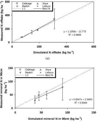
N offtake by the plant (excluding fibrous roots at harvest) and mineral N in the 1
top 90 cm of soil for the 4 crops were simulated and compared with the measured 2
values. Fig. 6 shows that the simulated data are not only highly correlated to, but also 3
almost proportional to the corresponding measured values for all crops. During the 4
simulations, no parameter values were adjusted to improve the fit between 5
measurement and simulation. This suggests that the model is properly constructed and 6
well parameterized for the tested conditions and is, therefore, able to make reasonable 7
predictions for the response of crop to N fertilizer, and N losses from the root zone by 8
leaching. 9
10
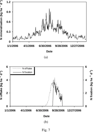
N dynamics in the different experiments was simulated and shown for the 11
soyabean experiment (see Fig. 7). The variation of N mineralization from soil organic 12
matter followed a similar pattern to the changes in air temperature, with the maximum 13
N mineralization occurring in summer (Fig. 7a). The simulated N mineralization rate 14
was 0.6 kg ha-1 d-1 at 20oC, close to the value of 0.7 kg ha-1 d-1 at 16oC derived from 15
the measurements on the same soil (Greenwood and Draycott, 1989). N offtake by the 16
crop increased with time in the early stages of growth, but decreased towards maturity. 17
This is a result of the dual action of a lower crop %N required for maximum growth 18
and a reduction in growth rate caused by lower temperatures in the later growth stages 19
(Fig. 7b). Soyabean is a crop capable of atmosphere-N fixation. When N supply from 20
the soil is limited, the crop fixes atmosphere-N to meet critical %N for the maximum 21
growth. Atmosphere-N fixation occurred only when the mineral N in the soil was 22
depleted to a minimum level below which no N uptake was possible, and thus started 23
at a later date than planting (Fig. 7b). A total of 148 out of the 205 kg-N ha-1 24
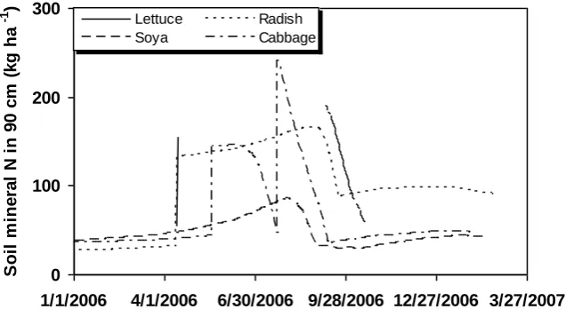
mineral N in the top 90 cm soil for different crops is plotted in Fig. 8. The sudden 1
increases in soil mineral N were due to the application of fertilizer-N, while the more 2
gradual increases were attributed to N mineralization from soil organic matter. The 3
sharp decreases in soil mineral N were the result of N uptake by crops. Since there 4
was no fertilizer-N applied to the soyabean crop, the mineral N in the top 90 cm soil 5
was general lower than those in other experiments. 6
7
All crops suffered from water stress to varying degrees as the accumulated 8
actual transpirations were less than the potential ones (Fig. 9). Radish suffered from 9
water stress most severely, whereas lettuce suffered the least. One contributory factor 10
to the high water stress of radish is that the crop was planted in the summer, when 11
rainfall was very sparse. The crop only grew for 27 days, and in the first 22 days the 12
crop lost a total of about 82.5 mm water by evapotranpiration. However, the water 13
infiltration in the same period was only 20 mm. Furthermore, radish is a shallow-14
rooted crop, which makes it less able to extract water from depth in the soil profile. 15
Compared with the other crops cabbage is a relatively deep-rooted species with a 16
fairly even root distribution (Thorup-Kristensen, 2006). This means the crop is able to 17
extract water from a bigger soil volume. Nevertheless, the total demand for 18
evapotranspiration during growth of cabbage of 491 mm was much greater than the 19
total water infiltration of 220 mm, resulting in shortage of soil water for the crop to 20
take up. This evidence suggests that the model is able to simulate water uptake 21
sensibly for various crop species. 22
23
Leaching mainly occurred in winter when rainfall was high and evaporative 24
significant leaching occurred during the summer when evapotranspirative demand 1
was high. This is supported by previous studies which showed that most leaching 2
occurs between late autumn and early spring, when the soil is not covered by crops in 3
European conditions (Neeteson and Carton, 2001). Since N leaching and water 4
percolation are coupled processes, the cumulative N leaching curves (Fig. 11b) have 5
the same trends as those in water losses (Fig. 11a). In both lettuce and radish 6
experiments, water percolation below 90 cm was greater, resulting from the relatively 7
short growth periods of these crops. This, together with higher mineral N 8
concentrations present in the soil (Fig. 8), led to greater N losses by leaching. The 9
cumulative N leaching in the lettuce and radish experiments was approximately 20 10
kg-N ha-1 by the end of simulations, about three times higher than that in the cabbage 11
and soyabean experiments. 12
13
5.4. Model evaluation 14
15
The improvement of modeling water dynamics in the soil-crop system has 16
been clearly demonstrated in reproducing the results from the PAGV experiment. The 17
predicted spatial-temporal soil water content using the updated model was in good 18
agreement with the measurements, whereas the original model could not satisfactorily 19
reproduce results in the deep soil where water content was greatly affected by 20
groundwater table. By employing the recently developed numerical scheme for the 21
basic soil water flow equation (Yang et al., 2009) in the updated model, the model not 22
only produced the identical results as those from the complex FE numerical scheme in 23
model capillary flow caused by high groundwater table, which has led to the 1
extension of the model application. 2
3
It is difficult to rigorously assess the performance of any crop N model on N 4
dynamics since N transfer in some processes such as N incorporation in roots is hard 5
to measure precisely. In this study it is even more difficult to do so because soil 6
mineral N was not frequently monitored in the experiments. However, some 7
assessment of the performance of the model on N dynamics is still possible based on 8
the following lines of evidence: 1) both the simulated values of N uptake in the above-9
ground dry weight in all the experiments and the mineral N in 90cm soil depth on the 10
measured dates were close to the measured values; 2) although the simulated N 11
incorporated in the roots could not be quantitatively validated because the 12
experimental data was unavailable, the approach for considering N partitioned in roots 13
has previously been proved acceptable for many crops (Zhang et al., 2009); 3) the soil 14
organic matter breakdown rate used was similar to those used in other models 15
(Mueller et al., 1996; Fang et al., 2005), and the simulated N mineralization rate of 0.6 16
kg ha-1 d-1 at 20oC was close to the value of 0.7 kg ha-1 d-1 at 16oC derived from the 17
measurements on the same soil (Greenwood and Draycott, 1989); 4) the simulated N 18
leaching from 90 cm soil depth was small during early spring and late autumn, which 19
was supported by the finding of Neeteson and Carton (2001); 5) N losses from the 20
processes such as ammonia volatilization and denitrification were not simulated, but 21
were previously found to be small in this sandy loam soil (Zhang et al., 2007, 2009). 22
23
Thus, it is reasonable to conclude that the updated model performed well in 24
is a need though to extend the functions of the model to simulate soil processes such 1
as denitrification, ammonia volatilization and ammonia fixation to further widen its 2
application. 3
4
6. Conclusions 5
6
A generic agro-hydrological model SMCR_N for the effect of N fertilizer on 7
crop growth and nitrate leaching has crucially been updated by replacing the existing 8
approximate hydrological algorithms with a simple and accurate approach based on 9
the basic flow equation. The updated model strikes a balance between accuracy, 10
simplicity and robustness. The model not only consistently out-performs the original 11
model in predicting internal water drainage in different soils and water dynamics in 12
the complex soil-wheat system, but also extends its use to the situations where the 13
capillary flow is important. Due to the highly accurate algorithm for hydrological 14
simulation, the updated model can now be employed for rigorous study of water 15
dynamics in the soil-crop system as well. 16
17
Validation of the updated SMCR_N model against data from field experiments 18
on 4 contrasting crops shows that the model is capable of reproducing the measured 19
data. The simulated results agree well with the measured values, indicating that the 20
updated SMCR_N model has been properly devised and parameterized. This, and its 21
validation against the comprehensive datasets of water and N measured in the wheat 22
experiments (Zhang, 2010) and the validation of the original model on 16 vegetable 23
and N use and assess the impact of N leaching from different management strategies 1
in crop production where diverse crops are grown. 2
3
Acknowledgements 4
5
The work was financed by EC and the UK Department for Environment, Food 6
and Rural Affairs through projects QLK5-CT-2002-01100 and HH3507SFV. The 7
authors are grateful to Dr J Neeteson for kindly providing the dataset for testing the 8
model. 9
References 1
2
Allen, R.G., Pereira, L.S., Raes, D., Smith, M., 1998. Crop evapotranspiration. 3
Guidelines for computing crop water requirements. FAO Irrigation and 4
Drainage Paper 56. FAO, Rome. 5
Bastiaanssen, W.G.M., Allen, R.G., Droogers, P., D’Urso, G., Steduto, P., 2007. 6
Twenty-five years modeling irrigated and drained soils: State of the art. Agri. 7
Water Manage 92, 111-125. 8
Bergstrom, L., Johnsson, H., Tortensson, G., 1991. Simulated nitrogen dynamics 9
using the SOILN model. Fert. Res. 27, 181–188. 10
Boone, A., Wetzel, P.J., 1996. Issues related to low resolution modeling of soil 11
moisture: Experience with the PLACE model. Global Planet. Change 13, 161-12
181. 13
Brisson, N., Gary, C., Justes, E., Roche, D., Zimmer, D., Sierra, J., Bertuzzi, P., 14
Burger, P., Bussière, F., Cabidoche, Y.M., Cellier, P., Debaeke, P., Gaudillère, 15
J.P., Hénault, C., Maraux, F., Seguin, B., Sinoquet, H., 2003. An overview of 16
the crop model STICS. Eur. J. Agron. 18, 309-332. 17
Burns, I.G., 1974. A model for predicting the redistribution of salts applied to fallow 18
soils after excess rainfall or evaporation. J. Soil Sci. 25, 165-178. 19
Burns, I.G., 1980. Influence of the spatial distribution of nitrate on the uptake of N by 20
plants: A review and a model for rooting depth. J. Soil Sci. 31, 155-173. 21
Cannavo, P., Recous, S., Parnaudeau, V., Reau, R., 2008. Modelling N dynamics to 22
Celia, M.A., Bouloutas, E.T., Zarba, R.L., 1990. A general mass-conservative 1
numerical solution for the unsaturated flow equation. Water Resour. Res. 26, 2
1483-1496. 3
Diekkruger, B., Sondgerath, D., Kersebaum, C.K., McVoy, C.W., 1995. Validity of 4
agroecosystem models: a comparison of results of different models applied to 5
the same data set. Ecol. Model. 81, 3–29. 6
Fang, C., Smith, P., Moncrieff, J.B., Smith, J.U., 2005. Similar response of labile and 7
resistant soil organic matter pools to changes in temperature. Nature 433, 57-59. 8
Fernández-Gálves, J., Simmonds, L.P., 2006. Monitoring and modelling the three-9
dimensional flow of water under drip irrigation. Agri. Water Manage 83, 197-10
208. 11
Gandolfi, C., Facchi, A., Maggi, D., 2006. Comparison of 1D models of water flow in 12
unsaturated soils. Environ. Model. Softw. 21, 1759-1764. 13
Greenwood, D.J., 2001. Modelling N-response of field vegetable crops grown under 14
diverse conditions with N_ABLE: A review. J. Plant Nutr. 24, 1799-1815. 15
Greenwood, D.J., Draycott, A., 1989. Experimental validation of an N-response 16
model for widely different crops. Fert. Res. 18, 153-174. 17
Greenwood, D.J., Gerwitz, A., Stone, D.A., Barnes, A., 1982. Root development of 18
vegetable crops. Plant Soil 68, 75-96. 19
Groot, J.J.R., Verberne, E.L.J., 1991. Response of wheat to nitrogen fertilization, a 20
data set to validate simulation models for nitrogen dynamics in crop and soil. 21
Fert. Res. 27, 349-383. 22
Hansen, S., Jensen, H.E., Nielsen, N.E., Svendsen, H., 1990. Daisy - A Soil Plant 23
Atmosphere System Model. NPO Research from the National Agency of 24
Hoogenboom, G., Wilkens, P.W., Thornton, P.K., Jones, J.W., Hunt, L.A., Imamura, 1
D.T., 1999. Decision support system for agrotechnology transfer v3.5. In: 2
Hoogenboom, G., Wilkens, P.W., Tsuji, G.Y. (Eds.), DSSAT Version 3, 3
Volume 4. University of Hawaii, Honolulu, HI (ISBN 1-886684-04-9), pp. 1-36. 4
Johnsson, H., Bergstrom, L., Jansson, P.-E., Paustian, K., 1987. Simulation nitrogen 5
dynamics and losses in a layered agricultural soil, Agri. Ecosyst. Environ. 18, 6
333-356. 7
Jones, J.W., Hoogenboom, G., Porter, C.H., Boote, K.J., Batchelor, W.D., Hunt, L.A., 8
Wilkens, P.W., Singh, W., Gijsman, A.J., Ritchie, J.T., 2003. The DSSAT 9
cropping system model. Eur. J. Agron. 18, 235-265. 10
Keating, B.A., Carberry, P.S., Hammer, G.L., Probert, M.E., Robertson, M.J., 11
Holzworth, D., Huth, N.I., Hargreaves, J.N.G., Meinke, H., Hochman, Z., 12
McLean, G., Verburg, K., Snow, V., Dimes, J.P., Silburn, M., Wang, E., Brown, 13
S., Bristow, K.L., Asseng, S., Chapman, S., McCown, R.L., Freebairn, D.M., 14
Smith, C.J., 2003. An overview of APSIM, a model designed for farming 15
systems simulation. Eur. J. Agron. 18, 235-266. 16
Lee, D.H., Abriola, L.M., 1999. Use of the Richards equation in land surface 17
parameterization. J. Geophys. Res. 104, 27519-27526. 18
Mualem, Y., 1976. A new model for predicting the hydraulic conductivity of 19
unsaturated porous media. Water Resour. Res. 12, 513-522. 20
Mueller, T., Jensen, L.S., Hansen, S., Nielsen, N.E., 1996. Simulating soil carbon and 21
nitrogen dynamics with the soil-plant-atmosphere system model Daisy, in: 22
Powlson, D.S., Smith, P., Smith, J.U. (Eds), Evaluation of Soil Organic Matter 23
Models Using Existing Long-Term Datasets. NATO ASI Series I, Vol. 38, 24
Neeteson, J.J., Carton, O.T., 2001. The environmental impact of nitrogen in field 1
vegetable production. Acta Horti. 563, 21-28. 2
Pedersen, A., Zhang, K., Thorup-Kristensen, K., Jensen, L.S., 2010. Modelling 3
diverse root density dynamics and deep nitrogen uptake – A simple approach. 4
Plant Soil 326, 493-510. 5
Rahn, C.R., Zhang, K., Lillywhite, R., Ramos, C., Doltra, J., de Paz, J.M., Riley, H., 6
Fink, M., Nendel, C., Thorup-Kristensen, K., Pedersen, A., Piro, F., Venezia, A., 7
Firth, C., Schmutz, U., Rayns, F., Strohmeyer, K., 2009. EU-Rotate_N – a 8
European decision support system – to predict environmental and economic 9
consequences of the management of nitrogen fertiliser in crop rotations. Eur. J. 10
Horti. Sci. 75, 20-32. 11
Ranatunga, K., Nation, E.R., Barratt, D.G., 2008. Review of soil water models and 12
their applications in Australia. Environ. Model. Softw. 23, 1182-1206. 13
Renaud, F.G., Bellamy, P.H., Brown, C.D., 2008. Simulation pesticides in ditches to 14
asses ecological risk (SPIDER): I. Model description. Sci. Total Environ. 394, 15
112-123. 16
Shao, Y., Henderson-Sellers, A., 1996. Modeling soil moisture: a project for 17
intercomparison of land surface parameterization schemes phase 2(b). J. 18
Geophys. Res. 101 (D3), 7227-7250. 19
Šimunek, J., Vogel, T., Van Genuchten, M.Th., 1992. The SWMS_2D code for 20
simulating water flow and solute transport in two-dimensional variably 21
saturated media, v 1.1, Research Report No. 126, U. S. Salinity Lab, ARS 22
USDA, Riverside. 23
Stöckle, C.O., Donatelli, M., Nelson, R., 2003. CropSyst, a cropping systems 24
Thorup-Kristensen, K., 2006. Root growth and nitrogen uptake of carrot, early 1
cabbage, onion and lettuce following a range of green manures. Soil Use 2
Manage. 22, 29-38. 3
Van Genuchten, M.Th., 1980. A closed-form equation for predicting the hydraulic 4
conductivity of unsaturated soils. Soil Sci. Soc. Am. J.44, 892-898. 5
Van Genuchten, M.Th., Leij, F.J., Yates, S.R., 1991. The RETC code for quantifying 6
the hydraulic functions of unsaturated soils. Robert S. Kerr Environmental 7
Research Laboratory, U. S. Environmental Protection Agency, Oklahoma, USA, 8
83pp. 9
Van Ittersum, M.K., Leffelaar, P.A., Van Keulen, H., Kropff, M.J., Bastiaans, L., 10
Goudriaan, J., 2003. On approaches and applications of the Wageningen crop 11
models. Eur. J. Agron. 18, 201-234. 12
Williams, J.R., Jones, C.A., Dyke, P.T., 1993. The Epic model. in: Sharpley A.N., 13
Williams J.R. (Eds.), Epic–Erosion Productivity Impact Calculator. 1. Model 14
documentation. U S Department of Agriculture Technical Bulletin No 1768. 15
USDA: Washington DC. 92 pp. 16
Wösten, J.H.M., Lilly, A., Nemes, A., Le Bas, C., 1999. Development and use of a 17
database of hydraulic properties of European soils. Geoderma 90, 169-185. 18
Yang, D., Zhang, T., Zhang, K., Greenwood, D.J., Hammond, J., White, P.J., 2009. 19
An easily implemented agro-hydrological procedure with dynamic root 20
simulation for water transfer in the crop-soil system: validation and application. 21
J. Hydrol. 370, 177-190. 22
Zhang, K., Greenwood, D.J., White, P.J., Burns, I.G., 2007. A dynamic model for the 23
combined effects of N, P and K fertilizers on yield and mineral composition; 24
Zhang, K., Yang, D., Greenwood, D.J., Rahn, C.R., Thorup-Kristensen, K., 2009. 1
Development and critical evaluation of a generic 2-D agro-hydrological model 2
(SMCR_N) for the responses of crop yield and nitrogen composition to nitrogen 3
fertilizer. Agri. Ecosyst. Environ. 132, 160-172. 4
Zhang, K., 2010. Evaluation of a generic agro-hydrological model for water and 5
nitrogen dynamics (SMCR_N) in the soil-wheat system. Agri. Ecosyst. Environ.. 6
doi: 10.1016/j.agee.2010.02.005.
7
Zhang, K., Burns, I.G., Greenwood, D.J, Hammond, J.P., White, P.J., 2010. 8
Developing a reliable strategy to infer the effective soil hydraulic properties 9
from field evaporation experiments for agro-hydrological models. Agri. Water 10
Manage. 97, 399-409. 11
Figure captions: 1
2
Fig. 1. Schematic representation of the model. The algorithms in the grey box are 3
implemented using a small time step 0.001d, while the other processes are 4
simulated using a time step of 1 d. 5
6
Fig. 2. Soil water content distributions simulated using different approaches for a 7
coarse soil (a) and a very fine soil (b) draining from saturation after 1d, 3d and 8
9d. Solid line represents the simulated results from the updated SMCR_N 9
model. Symbols open triangle and square represent the results from a finite 10
element (FE) method and the original SMCR_N model, respectively. 11
12
Fig. 3. Variation of the total water in a 200cm soil column with time calculated using 13
different approaches for a coarse soil (a) and a very fine soil (b) draining from 14
saturation. Solid line represents the simulated results from the updated 15
SMCR_N model. Symbols open triangle and square represent the results from 16
a finite element (FE) method and the original SMCR_N model, respectively. 17
18
Fig. 4. Overall comparison of soil water content down the profile at time intervals 19
between measurement and simulation using the original model and the 20
updated model in the PAGV experiment. Symbols open triangle and open 21
square represent the results from the original and updated models, respectively. 22
23
Fig. 5. Comparisons of soil water content in relation to the time DOY (day of the 24
models in the layers of 0 – 20 cm (a), 20 – 40 cm (b), 40 – 60 cm (c), 60 – 80 1
cm (d), and 80 – 100 cm (e) in the PAGV experiment. Solid and dotted lines 2
represent the simulations by the updated and original models, respectively. 3
Symbol open triangle represents the measurement. 4
5
Fig. 6. Comparisons between the measured and simulated N offtake in the plants 6
excluding fibrous roots (a) and mineral N in 90cm soil (b) for different crops. 7
The vertical bars represent the ranges of the measured values. 8
9
Fig. 7. Simulated daily N mineralization from soil organic matter (a) and N offtake 10
and N fixation (b) in the soyabean experiment. 11
12
Fig. 8. Simulated temporal changes in soil mineral N in the top 90 cm in different 13
experiments. 14
15
Fig. 9. Simulated cumulative potential (Tpot) and actual (Tact) transpiration for cabbage
16
and soybean (a), and lettuce and radish (b). 17
18
Fig. 10. Simulated daily water percolation and N leaching at 90 cm depth in the 19
soyabean experiment. 20
21
Fig. 11. Simulated cumulative water percolation (a) and N leaching (b) at 90 cm depth 22
in different experiments. 23
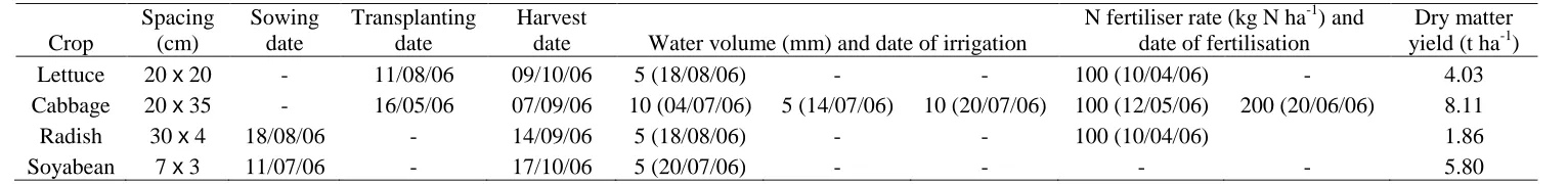
Table 1
Experimental details
Crop
Spacing (cm)
Sowing date
Transplanting date
Harvest
date Water volume (mm) and date of irrigation
N fertiliser rate (kg N ha-1) and date of fertilisation
Dry matter yield (t ha-1)
Lettuce 20 x 20 - 11/08/06 09/10/06 5 (18/08/06) - - 100 (10/04/06) - 4.03
Cabbage 20 x 35 - 16/05/06 07/09/06 10 (04/07/06) 5 (14/07/06) 10 (20/07/06) 100 (12/05/06) 200 (20/06/06) 8.11
Radish 30 x 4 18/08/06 - 14/09/06 5 (18/08/06) - - 100 (10/04/06) 1.86
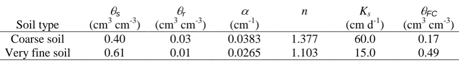
Table 2
Soil hydraulic properties used in the numerical experiments ( s, r, , n are the van
Genuchten soil hydraulic property parameters, representing the saturated and residual soil water content, the shape parameters of the retention and conductivity functions. Ks and FC are the saturated hydraulic conductivity and the soil water content at field
capacity, respectively)
Soil type
s
(cm3 cm-3)
r
(cm3 cm-3) (cm-1)
n Ks
(cm d-1)
FC
(cm3 cm-3)
Coarse soil 0.40 0.03 0.0383 1.377 60.0 0.17
Table 3
Fitted soil hydraulic properties in the PAGV experiment using the RETC software (van Genuchten et al., 1991) (See Table 2 for the meanings of the symbols in the Table)
Soil depth (cm)
s
(cm3 cm-3)
r
(cm3 cm-3) (cm-1)
n Ks
(cm d-1)
0–25 0.42 0.04 0.0162 1.299 160.0
25–40 0.50 0.06 0.0096 1.346 33.0
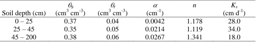
Table 4
Soil hydraulic properties in the soil profile in the validation experiments (See Table 2 for the meanings of the symbols in the Table)
Soil depth (cm)
s
(cm3 cm-3)
r
(cm3 cm-3) (cm-1)
n Ks
(cm d-1)
0 – 25 0.37 0.04 0.0042 1.178 28.0
25 – 45 0.35 0.05 0.0214 1.119 34.0
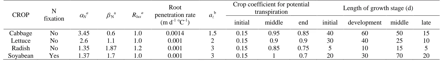
Table 5
Crop parameter values related to the maximum %N in the main (shoot and tap root) and root compartments, root development and transpiration
a
crop N nutrition coefficients in Eqs. (9), (10) and (15).
b
shape parameter for root length distribution down the soil profile in Eq. (12).
CROP N
fixation N
a
N a
Rlux a
Root penetration rate
(m d-1oC-1)
az b
Crop coefficient for potential
transpiration Length of growth stage (d)
initial middle end initial development middle late
Cabbage No 3.45 0.6 1.0 0.0014 1.5 0.15 0.95 0.85 40 60 50 15
Lettuce No 2.6 1.1 1.0 0.001 2 0.15 0.9 0.9 30 40 25 10
Radish No 1.35 1.87 1.2 0.001 3 0.15 0.85 0.75 5 10 15 5