Failure Rate Modeling Using Equipment Inspection Data

Failure Rate Modeling Using

Equipment Inspection Data

Richard E. Brown (SM)*

1Abstract—System reliability models typically use aver-age equipment failure rates. Even if these models are calibrated based on historical reliability indices, all like components within a calibrated region remain homo-geneous. This paper presents a new method of custom-izing failure rates using equipment inspection data. This allows available inspection information to be re-flected in system models, and allows for calibration based on interruption distributions rather than mean values. The paper begins by presenting a method to map equipment inspection data to a normalized condi-tion score, and suggests a formula to convert this score into failure probability. The paper concludes by apply-ing this methodology to a test system based on an ac-tual distribution system, and shows that the incorpora-tion of condiincorpora-tion data leads to richer reliability models. Keywords—predictive reliability assessment, equipment failure rate modeling, inspection-based ranking

I. INTRODUCTION

OWER DELIVERY COMPANIES are under increas-ing pressure to provide higher levels of reliability for lower cost. The best way to pursue these goals is to plan, engineer, and operate power delivery systems based on quantitative models that are able to predict expected levels of reliability for potential capital and operational strategies. Doing so requires both system reliability models and com-ponent reliability models.

Predictive reliability models are able to compute system reliability based on system topology, operational strategy, and component reliability data. The first distribution reli-ability model, developed by EPRI in 1978 [1], was not widely used due to conservative design and maintenance standards and, to a lesser extent, a lack of component reli-ability data. Eventually, certain utilities became interested in predictive reliability modeling and started developing in-house tools [2-5]. Presently, most major commercial cir-cuit analysis packages offer an integrated reliability mod-ule capable of predicting the interruption frequency and duration characteristics of equipment and customers. Ad-vanced tools have extended this basic functionality to in-clude momentary interruptions [6-7] and risk assessment [8-9].

*This paper is based on a paper of the same title to be published in IEEE Transactions on Power Systems. Richard Brown is with KEMA and can be reached at rebrown@ kema.com.

The application of predictive reliability models has tradi-tionally assigned average failure rate values to all compo-nents. Although simplistic, this approach produces useful results and can substantially reduce capital requirements while providing the same levels of predicted reliability [10]. Advanced tools have attempted to move beyond av-erage failure rates by either calibrating failure rates based on historical system performance [11], or by using multi-state weather models [12-13]. A few attempts have been made to compute failure rates as a function of parameters such as age [14], maintenance [15], or combinations of features [16], but these models tend to be system-specific and are not practicable for a majority of utilities at this time.

The use of average component failure rates in system re-liability models is always limiting and is potentially mis-leading [17]. Although generally acceptable for capital planning, the use of average values has two major draw-backs. First, average values cannot reflect the impact of relatively unreliable equipment and may overestimate the reliability of customers experiencing the worst levels of service. Second, average values cannot reflect the impact of maintenance activities and, therefore, preclude the use of predictive models for maintenance planning and overall cost optimization.

Most utilities perform regular equipment inspections and have tacit knowledge that relates inspection data to the risk of equipment failure. Integration of this information into component reliability models can improve the accuracy of system reliability models and extend their ability to reflect equipment maintenance in results.

Ideally, each class of equipment could be characterized by an equation that computes failure rate as a function of critical parameters. For example, power transformers might be characterized as a function of age, manufacturer, volt-age, size, through-fault history, maintenance history, and inspection results. Unfortunately, in most cases the sample size of failed units is far too small to generate an accurate model, and other approaches must be pursued.

This paper presents a practical method that uses equip-ment inspection data to assign relative condition rankings. These rankings are then mapped to a failure rate function based on worst-case units, average units, and best-case units. The paper then presents recommended failure rate models for a broad range of equipment, presents a method of calibration based on historical customer interruptions, and concludes by examining the impact of these techniques on a test system based on an actual distribution system.

II. INSPECTION-BASED CONDITION RANKING

Typical power delivery companies perform periodic in-spection on a majority of their electricity infrastructure. Utilities have various processes for collecting and re-cording inspection results. Paper forms stored in a multi-tude of departments make obtaining comprehensive system inspection results problematic. Many utilities, however, have migrated their inspection and maintenance programs to computerized maintenance management systems (CMMS) and data management systems that can be used as central warehouses for equipment inspection results.

After a population of similar equipment has been in-spected, it is desirable to rank their relative condition. Con-sider a piece of equipment with n inspection item results, (r1, r2 … , rn). Further suppose that each inspection item

result is normalized so that values correspond to the fol-lowing:

ri = 0 ; best inspection outcome

ri = ½ ; average inspection outcome

ri = 1 ; worst inspection outcome

Each inspection item result, ri, is assigned a weight, wi,

based on its relative importance to overall equipment con-dition. These weights are typically determined by the com-bined opinion of equipment designers and field service personnel, and are sometimes modified based on the par-ticular experience of each utility. The final condition of a component is then calculated by taking the weighted aver-age of inspection item results .By definition, a weighted average of 0 corresponds to the best possible condition, a weighted average of ½ corresponds to average condition, and a weighted average of 1 corresponds to the worst pos-sible condition.

∑

∑

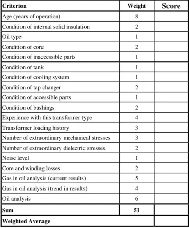
After each piece of equipment is assigned a condition score between 0 and 1, equipment using the same inspec-tion item weights can be ranked and prioritized for mainte-nance (typically considering cost and criticality as well as condition). This approach has been successfully applied to several utilities by the authors, and inspection forms and weights for most major pieces of power delivery equipment have been developed. In addition, inspection items have guidelines that suggest scores for various inspection out-comes. To illustrate, an inspection form for power trans-formers is shown in Table 1 and the scoring guideline for “Age” is shown in Table 2.

It should also be noted that inspection items can also be related to external factors. For example, overhead lines can include inspection items related to vegetation, animals, and lightning. Scores for these items will reflect both the exter-nal condition (e.g., lightning flash density) and system mitigation efforts (e.g., arrestors, shield wire, and ground-ing).

Although useful for prioritizing maintenance activities, relative equipment condition ranking is less useful for rig-orous reliability analysis. Since reliability assessment mod-els require equipment failure rates, inspection results would ideally be mapped into a failure rate through a closed-form equation derived from regression models. As mentioned earlier, this is not presently feasible for most classes of equipment due to limited historical data.

III. FAILURE RATE MODEL

Although there is not enough historical data to map in-spection results to failure rates through regression-based equations, interpolation is capable of providing approxi-mate results. At a minimum, interpolation requires failure rates corresponding to the worst and best condition scores. Practically, it requires one or more interior points so that non-linear relationships can be determined.

After exploring a variety of mapping functions, the au-thors have empirically found that an exponential model best describes the relationship between the normalized equipment condition of Eq. 1 and equipment failure rates. The specific formula chosen is:

Table 1. Inspection Form for Power Transformers

Criterion Weight Score

Age (years of operation) 8

Condition of internal solid insulation 2

Oil type 1

Condition of core 2

Condition of inaccessible parts 1

Condition of tank 1

Condition of cooling system 1

Condition of tap changer 2

Condition of accessible parts 1

Condition of bushings 2

Experience with this transformer type 4

Transformer loading history 3

Number of extraordinary mechanical stresses 3 Number of extraordinary dielectric stresses 2

Noise level 1

Core and winding losses 2

Gas in oil analysis (current results) 5 Gas in oil analysis (trend in results) 4

Oil analysis 6

Sum 51 Weighted Average

Table 2. Guideline for Power Transformer “Age”

Age (years of operation) Score

Less than 1 0.00

1 - 10 0.05

11 - 20 0.10

26-29 0.40 29-31 0.50 32-35 0.60 36-40 0.80 Greater than 40 1.00

( )

λ

Three data pairs are required to solve for the parameters A, B, and C. The previous section has developed a condi-tion ranking methodology that, by definicondi-tion, results in best, average, and worst condition scores of 0, ½, and 1, respectively. Therefore, three natural data pairs correspond to λ(0), λ(½), and λ(1). λ(½) can be approximated by tak-ing the average failure rate across many components or by using average failure rates documented in relevant litera-ture. λ(0) and λ(1) are more difficult to determine, but can be derived through benchmarking, statistical analysis, or heuristics. Given these three values, function parameters are determined as follows:

( ) ( )

[

]

( )

( ) ( )

( )

( )

( )

λ

λ

λ

λ

λ

λ

λ

λ

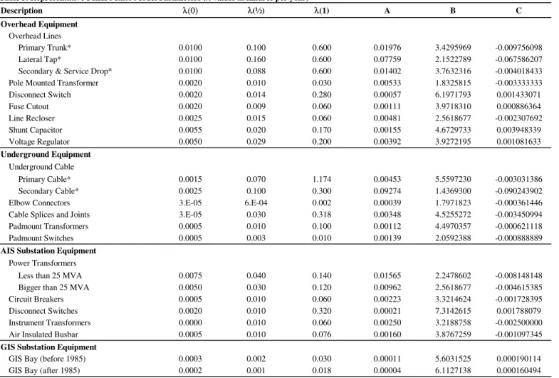
A detailed benchmarking of equipment failure rates is found in [18]. These results document low, typical, and high failure rates corresponding to system averages across a variety of systems. Assuming that (1) best-condition equipment have failure rates half that of best system aver-ages, (2) average-condition equipment have failure rates of typical system averages, and (3) worst-condition equip-ment have failure rates twice that of best system averages, parameters for a variety of equipment are shown in Table 3. These parameters, based on historical failure studies such as [14], are useful in the absence of system specific data, but should be viewed as initial conditions for calibra-tion, which is discussed in the next section.

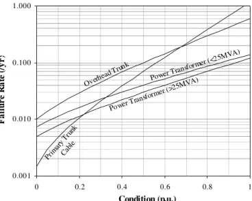
0.001 0.010 0.100 1.000 0 0.2 0.4 0.6 0.8 1 Condition (p.u.) F a il u r e R a te (/ y r) -Overh ead Tr unk Prim ary Tru nk Cab le Power T ransform er (<25M VA) Power T ransform er (>25M VA)

Figure 1. Selected Equipment Failure Rate Functions Failure rate graphs for some of the equipment in Table 3 are shown in Figure 1. These are simply plots of Eq. 2 us-ing the stated A, B, and C parameters the displayed equip-ment. It is interesting to see that the range of failure rates of certain types of equipment is large, while other types have a more moderate range. This reflects the ranges found in a broad literature search which forms the basis of Table 3.

IV. MODEL CALIBRATION

After creating a system reliability model, it is desirable to adjust component reliability data so that predicted sys-tem reliability is equal to historical syssys-tem reliability [11]. This process is called model calibration, and can be gener-alized as the identification of a set of parameters that mini-mize an error function.

Traditionally, reliability parameters (such as equipment failure rates) either remained uncalibrated or were adjusted based on average system reliability. For example, it may be known that an analysis area has an average of 1.2 interrup-tions per customer per year. Based on this number, failure rates can be adjusted until the predicted average number of customer interruptions is equal to this historical value. Af-ter failure rates are calibrated, switching and repair times can be adjusted until predicted average interruption dura-tion is also equal to historical values.

Calibrating based on system averages is useful, but does not ensure that the predicted distribution of customer inter-ruptions is equal to the historical distribution. That is, it does not ensure that either the most or least reliable cus-tomers are accurately represented – only that the average across all customers reflects history. This is a subtle but important point; since customer satisfaction is largely de-termined by customers receiving below-average reliability, calibration of reliability distribution is arguably more im-portant than calibration of average reliability.

A system model with homogeneous failure rates will produce a distribution of expected customer reliability lev-els (e.g., customers close to the substation will generally

have better reliability than those at the end of the feeder). If components on this same system are assigned random failure rates such that average system reliability remains the same, the variance of expected customer reliability will tend to increase. That is, the best customers will tend to get better, the worst customers will tend to get worse, and fewer customers can expect average reliability.

The distribution of expected customer reliability is criti-cal to customer satisfaction and should, if possible, be criti- cali-brated to historical data. A practical way to accomplish this objective is to calibrate condition-mapping parameters so that a distribution-based error function is minimized. Such an error function can be based on one of three levels of granularity: (1) individual customer reliability, (2) histo-grams of customer reliability, or (3) statistical measures of customer reliability.

An error function can be defined based on the difference between each customer’s historical versus predicted reli-ability. This approach calibrates reliability to the customer level and utilizes historical data at the finest possible

granu-Table 3. Representative Failure Rate Model Parameters (λ values in failures per year) Description λ(0) λ(½) λ(1) A B C Overhead Equipment Overhead Lines Primary Trunk* 0.0100 0.100 0.600 0.01976 3.4295969 -0.009756098 Lateral Tap* 0.0100 0.160 0.600 0.07759 2.1522789 -0.067586207

Secondary & Service Drop* 0.0100 0.088 0.600 0.01402 3.7632316 -0.004018433

Pole Mounted Transformer 0.0020 0.010 0.030 0.00533 1.8325815 -0.003333333

Disconnect Switch 0.0020 0.014 0.280 0.00057 6.1971793 0.001433071 Fuse Cutout 0.0020 0.009 0.060 0.00111 3.9718310 0.000886364 Line Recloser 0.0025 0.015 0.060 0.00481 2.5618677 -0.002307692 Shunt Capacitor 0.0055 0.020 0.170 0.00155 4.6729733 0.003948339 Voltage Regulator 0.0050 0.029 0.200 0.00392 3.9272195 0.001081633 Underground Equipment Underground Cable Primary Cable* 0.0015 0.070 1.174 0.00453 5.5597230 -0.003031386 Secondary Cable* 0.0025 0.100 0.300 0.09274 1.4369300 -0.090243902

Elbow Connectors 3.E-05 6.E-04 0.002 0.00039 1.7971823 -0.000361446

Cable Splices and Joints 3.E-05 0.030 0.318 0.00348 4.5255272 -0.003450994

Padmount Transformers 0.0005 0.010 0.100 0.00112 4.4970357 -0.000621118

Padmount Switches 0.0005 0.003 0.010 0.00139 2.0592388 -0.000888889

AIS Substation Equipment

Power Transformers

Less than 25 MVA 0.0075 0.040 0.140 0.01565 2.2478602 -0.008148148

Bigger than 25 MVA 0.0050 0.030 0.120 0.00962 2.5618677 -0.004615385

Circuit Breakers 0.0005 0.010 0.060 0.00223 3.3214624 -0.001728395

Disconnect Switches 0.0020 0.010 0.320 0.00021 7.3142615 0.001788079

Instrument Transformers 0.0000 0.010 0.060 0.00250 3.2188758 -0.002500000

Air Insulated Busbar 0.0005 0.010 0.076 0.00160 3.8767259 -0.001097345

GIS Substation Equipment

GIS Bay (before 1985) 0.0003 0.002 0.030 0.00011 5.6031525 0.000190114

GIS Bay (after 1985) 0.0002 0.001 0.018 0.00004 6.1127138 0.000160494

* Line and cable failure rates are per circuit mile

larity. However, historical customer reliability is stochastic in nature and will vary naturally from year to year. An er-ror function can be defined based on the difference be-tween each customer’s historical versus predicted reliabil-ity. This approach calibrates reliability to the customer level and utilizes historical data at the finest possible granularity. However, historical customer reliability is sto-chastic in nature and will vary naturally from year to year. This is especially problematic with frequency measures. Although customers on average may experience 1 interrup-tion per year, a large number of customers will not experi-ence any interruptions in a given year. Calibrating these customers to historical data is misleading, making about 10 years of historical data for each customer desirable. Unfor-tunately, most feeders change enough over 10 years to make this method impractical.

An error function can also use a histogram of customer interruptions as its basis. The historical histogram could be compared to the predicted histogram and parameters ad-justed to minimize the chi-squared error (χ2):

(

)

∑

−

=

h

p

h

χ

Where n is the number of bins, h is the historical bin value, and p is the predicted bin value. Using the chi-squared error is attractive since it emphasized the distribu-tion of expected customer reliability which is strongly cor-related to customer satisfaction. Histograms will vary sto-chastically from year to year, but the large number of cus-tomers in typical calibration areas prevent this from be-coming a major concern.

Last, an error function can be based on statistical meas-ures such as mean value (µ) and standard deviation (σ). The error function will typically consist of a weighted sum similar to the following:

(

)

(

)

β

σ

σ

µ

µ

α

Unlike the χ2 error, this function allows relative weights to be assigned to mean and variance discrepancies (α and β). For example, a relatively large a value will ensure that predicted average customer reliability reflects historical average customer reliability while allowing relatively large mismatches in standard deviation.

Once an error measure is defined, failure rate model pa-rameters can be adjusted so that error is minimized. Since this process is over determined, the authors suggest using Table 3 for initial parameter values and using gradient

de-scent or hill climbing techniques for parameter adjustment. Calibration is computationally intensive since error sensi-tivity to parameters must be computed by actual parameter perturbation, but calibration need only be performed once.

V. APPLICATION TO TEST SYSTEM

The methodologies described in the previous two sec-tions have been applied to a test system derived from an actual overhead distribution system in the Southern U.S. This model consists of three substations, 13 feeders, 130 miles of exposure, and a peak load of 100 MVA serving 13,000 customers. The analytical model consists of 4100 components.

Customer historical failures are computed from four-year historical averages. Equipment condition for this sys-tem was not available, and was therefore assigned for ran-domly for individual components based on a normal distri-bution with a 0.5 mean and a 0.2 standard deviation.

Calibration for this test system is performed based on the chi-squared error of customer interruptions. Initial fail-ure rates for all components are assigned based on λ(½) values in Table 3, and initial failure rates are computed based on condition and the parameters in Table 3. Calibra-tion is performed by a variable-step local search that guar-antees local optimality.

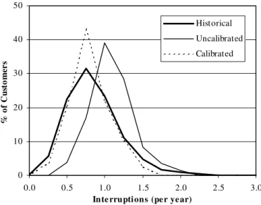
A summary of calibration results for overhead lines is shown in Figure 2, and a visualization of calibrated results in shown in Figure 3. The shape of the uncalibrated histo-gram is similar to the historical histohisto-gram, but with a mean and mode worse than historical values. After calibration, the modes align, but the predicted histogram retains a slightly smaller variance. In fact, the historical histogram is subject to stochastic variance, and the inability of the ex-pected value calibration to match this variance is immate-rial and perhaps beneficial.

Uncalibrated and calibrated failure rate parameters are shown in Table 4, and corresponding failure rate functions are shown in Figure 4. In effect, the calibration for this system did not change the failure rates for lines with good condition (less than 0.2), but drastically reduced the failure rates for lines with worse-than-average condition (greater than 0.5). These results are not unexpected, since this par-ticular service territory is relatively homogeneous in both terrain and maintenance practice, and extremely wide variations in overhead line failure rates have not been his-torically observed.

Table 4. Calibration Results for Overhead Line Parameters

Uncalibrated Calibrated A 0.01976 0.0170 B 3.429597 2.5981 C -0.00976 -0.00528 χ2 Error (%2) 1148.8 155.4 0 10 20 30 40 50 0.0 0.5 1.0 1.5 2.0 2.5 3.0

Inte rruptions (per year)

% o f Cu st o m er s Historical Uncalibrated Calibrated

Figure 2. Historical Versus Predicted Customer Interruptions

Figure 3. Visualization of Calibrated Results

0 0.1 0.2 0.3 0.4 0.5 0.6 0.7 0 0.1 0.2 0.3 0.4 0.5 0.6 0.7 0.8 0.9 1 Condition (p.u.) Fai lu re R a te (/ y r) Uncalibrated Calibrated

It is important to note that, in this case, equipment con-ditions were assigned randomly, and some were very high. Even though actual equipment for this system may never reach this poor condition state, the calibration process compensated by ratcheting down the failure rates assigned to equipment with the highest condition scores.

Once a system has been modeled and calibrated, it can be used as a base case to explore the impact of issues that may impact equipment condition such as equipment main-tenance. Once the expected impact that a maintenance ac-tion will have on inspecac-tion items is determined, the sys-tem impact of maintenance can be quantified based on the new failure rate. This allows the cost effectiveness of maintenance to be determined and directly compared to the cost effectiveness of system approaches such as new con-struction, added switching and protection, and system re-configuration.

VI. CONCLUSIONS

Equipment failure rate models are required for electric utilities to plan, engineer, and operate their system at the highest levels of reliability for the lowest possible cost. Detailed models based on historical data and statistical regression are not feasible at the present time, but this pa-per presents an interpolation method based on normalized condition scores and best/average/worst condition assump-tions.

The equipment failure rate model developed in this pa-per allows condition heterogeneity to be reflected in equipment failure rates. Doing so more accurately reflects component criticality in system models, and allows the distribution of customer reliability to be more accurately reflected. Further, a calibration method has been presented that allows condition-mapping parameters to be tuned so that the predicted distribution of reliability matches the historical distribution of reliability. Finally, the use of this condition-based approach allows the impact of mainte-nance activities on condition to be anticipated and reflected in system models, enabling the efficacy of maintenance budgets to be compared with capital and operational budg-ets.

This model is heuristic by nature, but adds a fundamen-tal level of richness and usefulness to reliability modeling, especially when parameters are calibrated to historical data. In the short run, gathering more detailed information on equipment failure rates and condition will strengthen this approach. In the long run, this same information can ultimately be used to develop explicit failure rate models that eliminate the normalized condition assessment re-quirement.

VII. REFERENCES

[1] EPRI Report EL-2018, Development of Distribution Reliability and Risk Analysis Models, Aug. 1981.

[2] S. R. Gilligan, “A Method for Estimating the Reliability of Distribu-tion Circuits,” IEEE Transactions on Power Delivery, Vol. 7, No. 2, April 1992, pp. 694-698.

[3] G. Kjolle and Kjell Sand, “RELRAD - An Analytical Approach for Distribution System Reliability Assessment,” IEEE Transactions on Power Delivery, Vol. 7, No. 2, April 1992, pp. 809-814.

[4] R.E. Brown, S. Gupta, S.S. Venkata, R.D. Christie, and R. Fletcher, “Distribution System Reliability Assessment Using Hierarchical Markov Modeling,” IEEE Transactions on Power Delivery, Vol. 11, No. 4, Oct., 1996, pp. 1929-1934.

[5] Y-Y Hsu, L-M Chen, J-L Chen, et al., “Application of a Microcom-puter-Based Database Management System to Distribution System Re-liability Evaluation,” IEEE Transactions on Power Delivery, Vol. 5, No. 1, Jan. 1990, pp. 343-350.

[6] C.M. Warren, “The Effect of Reducing Momentary Outages on Distri-bution Reliability Indices,” IEEE Transactions on Power Delivery,

Vol. 7, No. 3, July, 1992, pp. 1610-1615.

[7] R. Brown, S. Gupta, S.S. Venkata, R.D. Christie, and R. Fletcher, ‘Distribution System Reliability Assessment: Momentary Interruptions and Storms,’ IEEE PES Summer Meeting, Denver, CO, June, 1996. [8] R. E. Brown and J. J. Burke, “Managing the Risk of Performance

Based Rates,” IEEE Transactions on Power Systems, Vol. 15, No. 2, May 2000, pp. 893-898.

[9] L. V. Trussell, “Engineering Analysis in GIS,” DistribuTECH Confer-ence, Miami, FL, Feb. 2002.

[10] R. E. Brown and M. M. Marshall, “Budget-Constrained Planning to Optimize Power System Reliability,” IEEE Transactions on Power Systems, Vol. 15, No. 2, May 2000, pp. 887-892.

[11] R. E. Brown, J. R. Ochoa, “Distribution System Reliability: Default Data and Model Validation,” IEEE Transactions on Power Systems, Vol. 13, No. 2, May 1998, pp. 704-709.

[12] M. A. Rios, D. S. Kirschen, D. Jayaweera, D. P. Nedic, and R. N. Allan, “Value of security: modeling time-dependent phenomena and weather conditions,” IEEE Transactions on Power Systems, Vol. 17, No. 3 , Aug 2002, pp. 543 –548.

[13] R. N. Allen, R. Billinton, I. Sjarief, L. Goel, and K. S. So, “A Reliabil-ity Test System for Educational Purposes - Basic Distribution System Data and Results,” IEEE Transactions on Power Systems, Vol. 6, No. 2, May 1991.

[14] R. M. Bucci, R. V. Rebbapragada, A. J. McElroy, E. A. Chebli and S. Driller, “Failure Predic-tion of Underground Distribution Feeder Ca-bles,” IEEE Transactions on Power Delivery, Vol. 9, No. 4, Oct. 1994, pp. 1943-1955.

[15] D. T. Radmer, P. A. Kuntz, R. D. Christie, S. S. Venkata, and R. H. Fletcher, “Predicting vegetation-related failure rates for overhead dis-tribution feeders,” IEEE Transactions on Power Delivery, Vol. 17, No. 4, Oct. 2002, pp. 1170-1175.

[16] S. Gupta, A. Pahwa, R. E. Brown and S. Das, “A Fuzzy Model for Overhead Distribution Feeders Failure Rates,” NAPS 2002: 34th An-nual North American Power Symposium, Tempe, AZ, Oct. 2002. [17] J. B. Bowles, “Commentary-caution: constant failure-rate models may

be hazardous to your design,” IEEE Transactions of Reliability, Vol. 51, No. 3, Sept. 2002, pp. 375-377.

[18] R. E. Brown, Electric Power Distribution Reliability, Marcel Dekker, Inc., 2002.

VIII. BIOGRAPHIES

Richard E. Brown is a principal consultant with KEMA, and specializes in distribution reliability and asset management. He is the author or co-author of more than 50 technical papers and the book Electric Power Distribution Reliability. Dr. Brown received his BSEE, MSEE, and PhD from the Uni-versity of Washington and his MBA from the UniUni-versity of North Carolina at Chapel Hill. He is a registered professional engineer, and can be reached at [email protected].