Capital Mobility within EMU

econ

stor

www.econstor.eu

Der Open-Access-Publikationsserver der ZBW – Leibniz-Informationszentrum Wirtschaft

The Open Access Publication Server of the ZBW – Leibniz Information Centre for Economics

Nutzungsbedingungen:

Die ZBW räumt Ihnen als Nutzerin/Nutzer das unentgeltliche, räumlich unbeschränkte und zeitlich auf die Dauer des Schutzrechts beschränkte einfache Recht ein, das ausgewählte Werk im Rahmen der unter

→ http://www.econstor.eu/dspace/Nutzungsbedingungen nachzulesenden vollständigen Nutzungsbedingungen zu vervielfältigen, mit denen die Nutzerin/der Nutzer sich durch die erste Nutzung einverstanden erklärt.

Terms of use:

The ZBW grants you, the user, the non-exclusive right to use the selected work free of charge, territorially unrestricted and within the time limit of the term of the property rights according to the terms specified at

→ http://www.econstor.eu/dspace/Nutzungsbedingungen By the first use of the selected work the user agrees and declares to comply with these terms of use.

zbw

Working Paper

Capital Mobility within EMU

ZEW Discussion Papers, No. 99-19

Provided in cooperation with:

Zentrum für Europäische Wirtschaftsforschung (ZEW)

Suggested citation: Stirböck, Claudia; Heinemann, Friedrich (1999) : Capital Mobility within EMU, ZEW Discussion Papers, No. 99-19, http://hdl.handle.net/10419/24305

Capital Mobility within EMU

Claudia Stirböck and Friedrich Heinemann

Centre for European Economic Research (ZEW), Mannheim, Germany

April, 1999

Abstract:

Capital mobility is helpful to cope with the loss of adjustment instruments in EMU. High capital mobility in the sense of Feldstein and Horioka (FH) can limit the negative consequences of shocks affecting the saving capacity of an economy in the Euro zone. It is the aim of this paper to assess the likely degree of capital mobility in the FH sense within EMU. For this purpose, the FH approach is extended and updated. In particular, the role of current account targeting, exchange rate volatility and tax differentials as potential obstacles to capital mobility is analyzed. The empirical find-ings support the view that both current account targeting and exchange rate volatility were relevant for limiting the free flow of capital in the past. The conclusion is that within EMU domestic saving and investment will be less correlated than they were before the advent of the Euro.

Keywords: Capital Mobility, European Monetary Union, Investment-Saving-Relation JEL classification: F 36, F 21 Claudia Stirböck ZEW PO Box 10 34 43 D-68034 Mannheim Tel.: +49-621-1235-218 Fax: +49-621-1235-223 E-Mail: [email protected] Dr. Friedrich Heinemann ZEW PO Box 10 34 43 D-68034 Mannheim Tel.: +49-621-1235-149 Fax: +49-621-1235-223 E-Mail: [email protected]

I. Introduction

How mobile is capital internationally? Since Feldstein and Horioka (“FH”) (1980) found the degree of capital mobility among industrial countries in the period from 1960 to 1974 to be surprisingly low, this question has attracted a lot of interest. Inspite of an obviously fast pro-ceeding integration of financial markets the incomplete mobility according to the FH criterion was a result inspiring further research. At the end of the nineties, there is a constellation which makes this question particularly important. The introduction of a common currency in Europe changes the economic environment for policy making. The adjustable nominal ex-change rate is lost as an economic degree of freedom. Under the assumption that the nominal exchange rate can play a role as a helpful shock absorber, EMU makes the availability of other adjustment instruments desirable. Capital mobility is one of these potential adjustment instruments (Ingram, 1959).

In a world with perfect capital mobility in the FH sense, domestic investment does not depend on domestic saving: National savings feed a global saving pool out of which global invest-ment is financed. For a small country, changes in domestic saving are irrelevant for the level of domestic investment. The case is different with imperfect capital mobility which implies a direct link between domestic saving and investment. In this situation the degree of national investment depends on the saving capacity of the domestic households, enterprises and gov-ernment. Thus the degree of capital mobility is relevant for the question how member coun-tries of EMU will manage shocks affecting saving capacities asymmetrically. With perfect capital mobility the level of investment can be stabilized in a country with a negative devel-opment of saving capacity. The reduction of domestic saving is simply replaced by an in-crease of foreign capital inflow. On the other hand with imperfect capital mobility a decreas-ing domestic savdecreas-ing rate leads to a decrease of investment activity which negatively affects the growth and employment perspective of that country.

It is obvious that EMU and increasing monetary integration in Europe will have an impact on capital mobility. The end of nominal exchange rate risks eliminates one reason that often has been used to tell a story behind the „FH puzzle“. In order to draw conclusions for the avail-ability of an important adjustment instrument it would therefore be helpful to identify more clearly the role exchange rate variability played in the past as an obstacle to capital mobility. If it proves to be a major reason for the FH result, it would be justified to be optimistic con-cerning capital mobility in EMU.

This research was undertaken with support from the „Deutsche Post-Stiftung“ (German Mail Foundation) un-der the project „Arbeitsmarkteffekte un-der Europäischen Währungsunion“ (Labour Market Effects of European Monetary Union) as well as the “Deutsche Forschungsgemeinschaft” (German Science Foundation). Helpful comments from our colleagues Herbert S. Buscher and Thiess Büttner are gratefully acknowledged. We are also indebted to Ingo Sänger for excellent research assistance. All remaining errors are our own.

The degree of capital mobility in EMU might also be indirectly affected through taxation. EMU is expected to lead to increasing pressure on either politically negotiated or market in-duced tax harmonization. Steps to harmonize company taxation could possibly affect capital mobility and it would be helpful to learn something about the direction of this relation.

Finally, EMU will also change the objectives of economic policy. Politicians in Euroland which has a far lower degree of openness than the small European countries before will lose interest in exchange rate and current account developments. Particularly the latter is an im-portant change in the context of the FH debate. One explanation for the FH result is the idea that governments follow a strategy of current account targeting. Through the use of fiscal or other instruments governments try to balance the current account in the medium term (Bayo-umi, 1990; Summers, 1988). If this is the case this would explain a low degree of capital mo-bility in the FH sense. Because EMU makes current account balancing a largely senseless strategy for a single Eurozone member country this would also hint of an increasing degree of capital mobility from 1999 onwards.

With this in mind, it is the aim of this paper to assess capital mobility within EMU by ana-lyzing the importance of current account targeting, tax burden differentials and exchange rate variability for the FH results. If it can be shown that current account targeting and exchange rate volatility have some explanatory power for a low degree of capital mobility in the past, the emerging conclusion is that EMU will indeed increase capital mobility in the FH sense. The structure of the paper is as follows. In section 2 there is a short survey on the original FH approach and the literature emanating from the FH discussion. A particular focus will be on the main criticism that has come up in the discussion of the “FH puzzle” and on the impact of economic integration and exchange rate fluctuations. Section 3 includes an update of the original FH approach for the OECD countries until the latest available year (1996). Section 4 changes the focus from aggregate to private saving and investment ratios: This modification is to supply evidence on the role of current account targeting. In section 5, the impact of tax differentials and nominal exchange rate variability on capital mobility is analyzed. In the final section, the conclusions for the likely degree of capital mobility under EMU are drawn.

II. Survey and Main Criticism on Feldstein and Horioka

The FH approach is based on a simple relation. In a closed economy domestic investment is equal to domestic saving by definition. In an open economy a deviation from this identity is possible as domestic investments can be financed by foreign savings to the extent capital is mobile. Therefore, FH interprete the correlation of domestic saving and domestic investment as an indicator for the degree of capital mobility.

FH are aware about the fact that simultaneous capital ex- and imports can exist because of strategic reasons such as international diversification. They focus, however, on net flows.

Capital mobility in their sense is the international mobility of the world’s supply of capital. This means that in the case of perfect mobility each additional unit of savings is invested worldwide at the place with the highest return. International capital flows should then respond to country differences in saving rates. Under perfect capital mobility the correlation of do-mestic saving rates and investment rates should be zero since additional dodo-mestic savings do not increase domestic investment but go to a global saving pool out of which investment is financed worldwide. If instead capital is totally immobile, the correlation is one, because each additional unit of saving is invested at home.1

In the original study, FH took data from the OECD National Accounts for 16 industrialized countries and ran their regressions for the time period from 1960 to 1974.2 The saving-investment correlation is analyzed in the context of the following cross section equation by the use of three five-year-averages as well as the total period average of the ratio of gross do-mestic saving to gross dodo-mestic product (GDP) and gross dodo-mestic investment to GDP:

(I/Y) i = α + β (S/Y) i with i being the country index.

β can be interpreted as the saving retention coefficient as it represents the share of the saving ratio invested at home. This coefficient is the indicator for capital mobility in the FH sense. A

β of zero (of one) indicates perfect (the absence of any) capital mobility.

FH find β equal to 0.89 (s.e. = 0.0.7) for the 15-year period while this coefficient falls from 0.909 (s.e. = 0.06) to 0.871 (s.e. = 0.09) in the 5-years-subperiods. The saving retention coef-ficient is in no case significantly different from 1. An increase in domestic saving does not seem to be invested internationally but domestically. The conclusion is that capital mobility is surprisingly low.

These results are a provocation to the widespread view that global financial integration has been proceeding fast since the sixties. This sense of provocation is more vivid at the end of the nineties when terms like “internationalization” and “globalization” have advanced to something like a creed for economic policy makers. The finding of a relatively low degree of capital mobility stands in a striking contrast to the fact that financial markets due to the im-provement of communication technology, the development of new products and the abolition of capital controls are integrating at a fast pace.

1

Nevertheless, a correlation of one is only a necessary but not a sufficient condition for perfect capital immobil-ity. In the case of simultaneous capital in- and outflows, the correlation can for example be one though interna-tional capital flows exist. A correlation below one, however, clearly indicates some degree of capital mobility.

2

FH make use of the ratio of gross domestic investment to gross domestic product as well as of the ratio of gross domestic saving to gross domestic product.

The results might not be that surprising, however, if one considers the obstacles to the mobil-ity of short-run financial capital on the one hand and of long-run portfolio capital or direct investment on the other hand. In the short run, the regulatory framework concerning capital restrictions or differential tax treatments can be regarded as stable. Furthermore, markets for the hedging of exchange rate risks exist and are highly liquid. For a long-run investor, the situation is different, because the politically determined environment can not be assumed to be stable. If there are no capital restrictions today, obstacles to the repatriation of capital or unfavorable treatment of foreigners could be introduced again at some point in the future. Hedging exchange rate risks on the long run is often not possible. Even if it is possible, it is likely to be relatively expensive due to the lower liquidity of long term in comparison to short term forward markets. Thus, in principle, a low degree of capital mobility in the FH sense is possible, even if financial integration is perfect in the light of the (short-run) covered interest parity condition.

Different lines of criticism have, nevertheless, been put forward against the FH approach (for a summary of the criticism see Lemmen and Eijffinger, 1995. Obviously, there is an endoge-neity problem in regressing investments on savings. In the original paper, the authors have been well aware of this problem and made use also of a two stage least squares approach in a simultaneous equation framework with a specified saving function. The results of the simple OLS estimation proved to be robust.3 Apart from that, the use of suitable period averages is able to decrease the problem of endogeneity along business cycles.

The calculation of averages might, however, lead to another problem. Due to the intertempo-ral budget restriction of an economy, current account deficits should on the long run add up to zero.4 Since the difference between domestic investment and saving is the current account deficit, a high correlation between both variables coming out of a regression based on long run period averages could simply reflect the fact that a country can not permanently increase its foreign debt. Using long run averages thus may imply a bias for finding a low degree of capital mobility (Sinn, 1992). This argument has also been used in a slightly modified manner (Summers, 1988) which is important in the EMU context: Governments often include the cur-rent account to the list of policy objectives. In this case they will employ suitable policy in-struments to improve the current account in the situation of large deficits. Thus the FH find-ing of a high correlation between savfind-ing and investment might simply reflect a political strat-egy of current account targeting. If this is the case, EMU will improve capital mobility

3

In this context, FH made use of several instrumental variables in different combinations: the growth rate of total private income, the ratio of the number of retirees over the age of 65 to the population aged 20 to 65, the ratio of the number of younger dependants to the working age population, the benefit-earnings replacement ratio as well as the labour force participation rate of older men. Testing for linearity, they found no evidence of non-linearity in the saving-investment correlation. Also, the rate of population growth potentially having a strong impact on the saving rate did not exert a statistically significant effect on the investment rate while the original saving retention coefficient remained almost constant.

4

This is a very approximate statement, since real growth rate and interest rates of an economy have to be taken into account to calculate a sustainable current account deficit, which could well be positive for long periods.

cording to the FH concept because under EMU current account targeting is a very unlikely strategy for national policy makers. Within a monetary union the current account restriction ceases to be a restriction because negative consequences of large deficits such as exchange rate crises are no longer feasible.

Finally, the FH measure for capital mobility is only adequate as long as the small country assumption holds. A large country will experience an impact of its saving ratio on its invest-ment ratio because the domestic saving ratio is of relevance for the world level of interest rates and thus for world investment. This problem, however, will probably be relevant only for very large economies like the USA or Japan.

One or the other, however, both the FH methodological approach and the main findings have survived its critiques. This is the reason why it seems adequate to use this measure for an analysis of the development of the degree of capital mobility and EMU’s influence on it. The impact of economic integration and the exchange rate regime on capital mobility ac-cording to the FH criterion has been touched in a couple of papers but remains unresolved. From a long run perspective, Hogendorn (1998) shows that capital mobility has fluctuated considerably in the last 150 years. It was highest during the decade 1905-1914, the zenith of the classical gold standard. In contrast to that, the Bretton Woods era was characterized by a saving retention coefficient of 1, i.e. complete immobility of capital. After the end of the Bretton Woods system capital mobility increased again (see also Feldstein/Bacchetta, 1991), it has however not yet reached again the levels of the period before World War. The increas-ing capital mobility after the end of fixed exchange rate is an interestincreas-ing result in regard to EMU since it contradicts the view that exchange rate certainty is a substantial accelerator of capital mobility. In contrast to this, Bhandari/Mayer (1990) find the EMS to have a positive influence on capital mobility of its member countries. Generally, a deepening of economic integration as it is under way in Europe is expected to increase financial flows (Feld-stein/Bacchetta, 1991; Artis/Bayoumi, 1991), although Dornbusch (1991) on the basis of data 1960-1986 fails to find a significant European Community effect.

Helliwell and McKitrick (1998) focus on capital mobility on the level of Canadian provinces and find that correlation between savings and investment disappears among provinces whereas it is significant on the national level. They ascribe this findings vaguely to barriers to trade and investment associated with national borders. Thus it remains unanswered which particular characteristics of a national border hinder the flow of capital. A more precise iden-tification is, however, necessary to assess capital mobility within EMU since the Euro zone is a mixed case between a unified economy and a group of sovereign countries.

III. Updating Feldstein Horioka

According to conventional wisdom, the nineties have sped up the process of globalization. In Europe, the years since 1990 have shown different developments relevant for capital mobility. The period 1992-1995 has been a turbulent time on foreign exchange markets. Within the

EMS, there were several crises with a high volatility of exchange rates. While these events might have negatively affected capital mobility, the completion of the internal market 1993 should have had a positive impact. Therefore, an update of the FH is necessary.

In comparison to the original FH work, data for Iceland, Portugal and Turkey are included, data for Luxemburg are excluded.5 The following subgroups are used:

• Core: includes the DM-zone countries Austria, Belgium, Denmark, France, West Germany

and the Netherlands

• Rest of EU: includes Finland, Great Britain, Greece, Italy, Portugal, Spain, Sweden and

Ireland

• Rest of the world: includes Australia, Canada, Iceland, Japan, Norway, New Zealand,

Switzerland, Turkey and the USA.

Investment ratios are calculated by dividing gross fixed capital formation by GDP.6 Gross saving ratios are calculated by dividing net savings plus consumption of capital by GDP. Data originate from the OECD National Accounts. Time series for saving and investment ratios are shown in the Appendix I (Illustration 1).

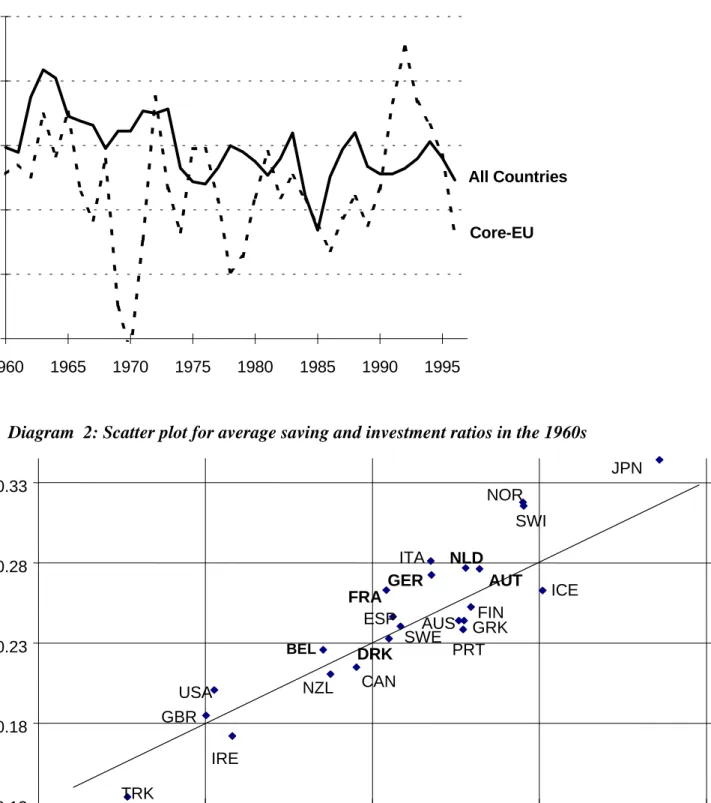
In order to limit the impact of business cycle effects period averages are used in the FH analy-sis. As an illustration, table A1 in Appendix II gives yearly saving retention coefficients of annual cross-sectional regressions for two country-groups, all countries and the subgroup EU core countries.7 On the basis of these estimations diagram 1 presents the saving retention co-efficients for all countries and EU core countries from 1960 to 1996. The saving-investment correlation coefficients actually show a high annual variability. The correlation is not con-stantly at a high degree, but seems to underlie itself cyclical influences.

5

It does not seem to be sensible to include the outlier Luxemburg with its specific characteristics of a small country with a huge financial market place.

6

All variables have been constructed in the same way as in the original FH approach. Although instead of “Gross Domestic Investment” “Gross Fixed Capital Formation” was taken in order to avoid arbitrary fluctua-tions in stocks. Bayoumi (1990) has used both concepts but found the regression results to be very similar.

7

As the cross-section regressions for the subgroup of EU core countries only contains 6 observation points, the regression results should be interpreted very carefully.

Diagram 1: Development of saving retention coefficients of yearly cross-sectional regressions. 0 0,2 0,4 0,6 0,8 1 1960 1965 1970 1975 1980 1985 1990 1995 Core-EU All Countries

Diagram 2: Scatter plot for average saving and investment ratios in the 1960s

0.13 0.18 0.23 0.28 0.33 0.13 0.18 0.23 0.28 0.33 Investment Ratio TRK GBR USA IRE BEL NZL CAN DRK FRA SWE ESP JPN ICE SWI NOR ITA GER AUT PRT GRK AUS FIN NLD Saving R a ti o

Diagram 3: Scatter plot for average saving and investment ratios in the 1980s 0.13 0.18 0.23 0.28 0.33 0.13 0.18 0.23 0.28 0.33 Investment Ratio Saving Ratio JPN PRT SWI FIN AUT AUS GRK NZL ICE IRE NLD GER ITA CAN TRK ESP FRA SWE USA DRK GBR BEL NOR

Note: EU core countries are presented in bold letters

Diagram 4: Scatter plot for average saving and investment ratios in the 1990s

0.13 0.18 0.23 0.28 0.33 0.13 0.18 0.23 0.28 0.33 Investment Ratio Saving Ratio JPN SWI AUT PRT TRK NOR NLD GER ESP GRK AUS FRA BEL CAN NZL FIN ITA IRE DRK ICE GBR USA SWE

Diagrams 2-4 present the position of 23 industrial countries regarding the correlation between saving and investment ratios of different time averages. A position on the 45-degree-line rep-resents complete immobility of capital in the FH sense. These diagrams already hint on in-creasing capital mobility after the sixties.

Table 1 and 2 summarize results of the update of the FH approach. The tables present saving retention coefficients as they result from the basic FH regression (see above section 2) based on a cross section of period averages. Table 1 reports results for five-year-averages and table 2 for ten-year averages. The coefficients in these tables are regarded with respect to their sig-nificant difference from zero.

Table 1: Saving retention coefficients (FH regression based on five-year averages)8

ALL COUNTRIES 1960-1964 0.737 *** 1965-1969 0.674 *** 1970-1974 0.685 *** 1975-1979 0.594 *** 1980-1984 0.572 *** 1985-1989 0.539 *** 1990-1994 0.562 *** no. of observ. 23

*/**/***: indicating that the coefficient is significant at the 10/5/1 percent level.

Table 2: Saving retention coefficients (FH regression based on ten-year averages)9

ALL COUNTRIES 1960-1969 0.708 *** 1970-1979 0.666 *** 1980-1989 0.553 *** 1990-1996 0.532 *** no. of observ. 23

*/**/***: indicating that the coefficient is significant at the 10/5/1 percent level.

For the 23 OECD countries, the results show the expected pattern. From the sixties onwards a long run tendency to a lower correlation between domestic investment and saving is observed. In comparison to the FH results, the estimations show a smaller β, even in 1960-64, 1965-69 and 1970-74. Additionally, the saving retention coefficients are significantly different from unity according to the Wald-Test. Although far from being perfect it seems that the interna-tional mobility of capital in the FH sense is increasing, especially in the 1980s and 1990s.

8

Detailed results can be found in Appendix II Table A2.

9

Due to the small number of observations (one observation per country per subperiod), period average regressions for subgroups would show a low degree of significance. In order to achieve correlations for the same time periods, but different country groups, while including a sufficient number of observations, the FH relation is explored by time series cross section regressions of the following type10:

(I/Y) i t = α + β (S/Y) i t

with i being the country index and t the time index.

This specification is also helpful in order to check the robustness of the period average results against the criticism by Sinn (1992) that - due to long-run limitations on foreign indebtedness - period averages tend to bias the saving retention coefficient towards 1.

In order to control for the bias resulting from the business cycle in the use of annual data, the given specification is estimated both with the usual, non adjusted, (table 3) and cyclically adjusted (table 3a) annual data for the five-year periods.11 For the estimation based on ten-year periods only results without cyclical adjustment are reported.

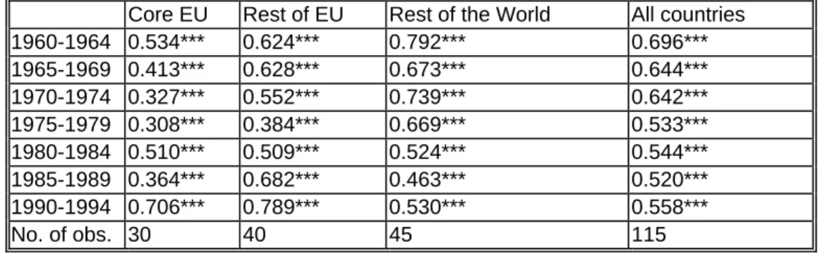
Table 3: Saving retention coefficients (panel estimation, five-year periods) 12

Core EU Rest of EU Rest of the World All countries 1960-1964 0.534*** 0.624*** 0.792*** 0.696*** 1965-1969 0.413*** 0.628*** 0.673*** 0.644*** 1970-1974 0.327*** 0.552*** 0.739*** 0.642*** 1975-1979 0.308*** 0.384*** 0.669*** 0.533*** 1980-1984 0.510*** 0.509*** 0.524*** 0.544*** 1985-1989 0.364*** 0.682*** 0.463*** 0.520*** 1990-1994 0.706*** 0.789*** 0.530*** 0.558*** No. of obs. 30 40 45 115

*/**/***: indicating that the coefficient is significant at the 10/5/1 percent level.

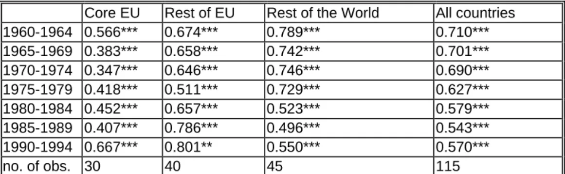
Table 3b: Saving retention coefficients

10

While previous studies in general concentrated on cross-country estimations, Vamvakidis and Wacziarg (1998) is another study analyzing panel estimations. This research also controls for fixed effects in this context since country-specific effects might be correlated with the domestic saving rate and thus bias the saving reten-tion coefficient. Vamvakidis and Wacziarg hereby find roughly the same results than in their cross-secreten-tional analysis. The use of this method therefore does not seem to change or even to bias the results. In our analysis, we, however, do not make use of fixed effects in order to avoid further problems of insufficient observation points.

11

In order to get cyclically adjusted data, a trend variable of the original data was created by use of the Hodrick Prescott Filter of 10. The use of a filter of 10 and not of 100 was motivated by the highly smoothing effect of the filter of 100.

12

(panel estimation based on cyclically adjusted data, five-year periods) 13

Core EU Rest of EU Rest of the World All countries 1960-1964 0.566*** 0.674*** 0.789*** 0.710*** 1965-1969 0.383*** 0.658*** 0.742*** 0.701*** 1970-1974 0.347*** 0.646*** 0.746*** 0.690*** 1975-1979 0.418*** 0.511*** 0.729*** 0.627*** 1980-1984 0.452*** 0.657*** 0.523*** 0.579*** 1985-1989 0.407*** 0.786*** 0.496*** 0.543*** 1990-1994 0.667*** 0.801** 0.550*** 0.570*** no. of obs. 30 40 45 115

*/**/***: indicating that the coefficient is significant at the 10/5/1 percent level.

Table 4: Saving retention coefficients (panel estimation, ten-year periods)14

Core EU Rest of EU Rest of the World All countries 1960-1969 0.499 *** 0.625 *** 0.732 *** 0.677 ***

1970-1979 0.413 *** 0.455 *** 0.679 *** 0.565 *** 1980-1989 0.428 *** 0.587 *** 0.490 *** 0.530 *** 1990-1996 0.652*** 0.715*** 0.511*** 0.543 *** no. of obs. 60 (40) 80 (56) 90 (63) 230 (159)

*/**/***: indicating that the coefficient is significant at the 10/5/1 percent level.

Numbers of observations in brackets relate to time period 1990 - 1996.

These results on the basis of the panel estimation show that the findings according to the original FH period average approach are robust. The panel estimation coefficients for all countries are in fact smaller than the period average estimation coefficients. It seems that the latter actually tend to be biased towards one. But the similarity of the estimation results of tables 1 and 3 as well as tables 2 and 4 proves that cross section time series estimations are not biased by business cycles. Additionally, the fact that the results of tables 3 and 3a are not very different also indicates that cyclical movements do not affect the correlation systemati-cally.

The estimation results again show a tendency to a lower correlation between domestic saving and investment, i.e. increasing capital mobility, from 1960 to 1990. It is also not surprising that for most subperiods the correlation is lower for the European core countries than for the rest of EU or the rest of the world. It is, however, striking that the correlation is increasing again in the 1990s, an effect particularly strong in the European core countries. The conse-quence is that correlations in the nineties are higher in Europe than in the rest of the world.

13

Detailed results can be found in Appendix II Table A5.

14

IV. The Role of Current Account Targeting

After the introduction of a single European currency the sustainability of internal current ac-counts within Euroland ceases to be a restriction for national economic policy. This was dif-ferent before. Under the EMS regime, due to the potential effects on exchange rates attention was paid to current account developments. Therefore, the presumption is that current account targeting could be the main reason behind the finding of low capital mobility in industrial countries. Current account targeting could also possibly be the explanation for the reversion to a higher correlation between saving and investment in Europe in the nineties. As a conse-quence of exchange rate turbulences attempts to balance the current account might have been intensified in the nineties. If this presumption is supported by the data, the conclusion for capital mobility within EMU is straightforward: it will increase.

If current account targeting existed, the saving retention coefficient of the private sector should differ from the coefficient of the total economy. More precisely, current account tar-geting might take place if the mobility of private capital is higher than the one of aggregated domestic capital.15 This refers to a lower private saving retention coefficient. Bayoumi (1990) using a sample of 10 OECD countries already found a lower correlation for private sector data and concluded that either structural reasons or economic policy must cause this phenomenon.

In order to derive private sector investment and saving, shown in Appendix I Figure 2, gen-eral government investment (gengen-eral government saving) had to be subtracted from total fixed investment (total saving).16

As general government sector data were rarely available from 1960 on, regressions start in 1970. Also, the group-specific estimates have to be modified as government data are not available for all 23 countries. Therefore, estimations are run for the core countries of EU (be-ing Germany, Belgium, Denmark and France, as well as Austria from 1975 on and the Neth-erlands from 1980 on) as well as all countries being 15 altogether (6 core countries plus Aus-tralia, Canada, Finland, Japan and UK as well as from 1980 on Italy, Norway, Sweden and USA).

15

Hereby attention has to be paid to the fact that government investment is not only financed by government saving. As instead government investment often exceed government saving, savings are deprived of the private sector. As a consequence, the correlation of private investment and private saving might a priori be lower than 1.

16

In the OECD National Accounting System general government saving is defined as general government cur-rent receipts minus general government curcur-rent disbursement. Therefore, general government saving can be negative saving if current disbursement (not including spending on investments) of the government exceeds its returns. Although these OECD data are standardized, country-specific characteristics cannot always be ex-cluded.

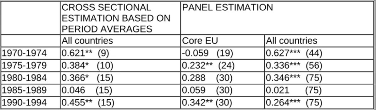
Table 5: Saving retention coefficients for private sector data for five-year periods17

CROSS SECTIONAL ESTIMATION BASED ON PERIOD AVERAGES

PANEL ESTIMATION

All countries Core EU All countries 1970-1974 0.621** (9) -0.059 (19) 0.627*** (44) 1975-1979 0.384* (10) 0.232** (24) 0.336*** (56) 1980-1984 0.366* (15) 0.288 (30) 0.346*** (75) 1985-1989 0.046 (15) 0.059 (30) 0.021 (75) 1990-1994 0.455** (15) 0.342** (30) 0.264*** (75)

*/**/***: indicating that the coefficient is significant at the 10/5/1 percent level. Number of observations is given in brackets.

Table 6: Saving retention coefficients for private sector data for ten-year periods18

CROSS SECTIONAL ESTIMATION BASED ON PERIOD AVERAGES

PANEL ESTIMATION

All countries Core EU All countries 1970-1979 0.523** (9) 0.098 (46) 0.504*** (100) 1980-1989 0.196 (15) 0.118 (60) 0.147** (150) 1990-1995 0.471** (15) 0.339** (35) 0.248*** (87)

*/**/***: indicating that the coefficient is significant at the 10/5/1 percent level.

Number of observations is given in brackets.

For private sector investment and saving, saving retention coefficients are systematically lower than for total saving and investment. In the 1980s, coefficients are not significantly different from zero indicating a high degree of capital mobility. These findings suggest that current account targeting has been relevant. Unbalanced current accounts of the private sector tend to be balanced by compensatory government activity. The reversion from high to low capital mobility from the 1980s to the 1990s can, however, also be detected in the private sector data. However, private sector data correlation in the EU core countries is not very dif-ferent from private sector data correlation regarding all countries while the correlation of total savings and investment was much higher in the EU countries than in the non-EU countries. An explanation for the surprisingly low capital mobility in the first half of the 1990s particu-larly strong in the EU countries could therefore come from increasing capital account target-ing of the EU governments. Such a policy behavior can be due to the higher exchange rate volatility in this period, a hypothesis analyzed in the following section.

17

Detailed results can be found in Appendix II Table A 7.

18

V. Impact of Exchange Rate Variability and Taxation

With EMU, European monetary integration will change the economic environment concern-ing exchange rate movements and possibly taxation. By definition nominal exchange rate fluctuations that have influenced economic decisions in the past will be eliminated inside EMU by definition. As this volatility is supposed to have exerted negative impacts e.g. on foreign direct investment and investment abroad, exchange rate stability might increase the international mobility of capital in the future. Therefore, it is important to identify the effect of exchange rate volatility on capital flows in the past. If it actually represented an obstacle to the international mobility of the supply of capital, the increasing capital mobility could play a more important role as a stabilizer in EMU than in the past. The impact of EMU on taxation is of a more indirect nature. It can be expected that the single currency will intensify tax compe-tition which again may speed up tax harmonization. If tax differentials are relevant for the mobility this could be another channel through which EMU affects capital mobility.

The impact of exchange rate volatility and tax differentials on capital mobility is analyzed in the context of an extended FH equation. In order to measure the influence of the economic openness on the saving-investment correlation, FH used a similar extension in their original paper of the following form:

(I/Y)i = α + (β0 + β1* Xi)*(S/Y) i with i being the country index.

This statistical specification allows the saving retention coefficient to vary according to the influence of different measures of economic openness Xi.19 The same econometric approach is used in the following regarding the effect exerted by exchange rate volatility and tax differ-entiation on capital mobility.

First, the analysis of the influence of exchange rate volatility focuses on the 19 industrialized countries20 for which data of the external value of their currencies against the other 18 coun-tries has been available from the German Bundesbank. In order to obtain measures of the de-gree of volatility of these currencies, yearly standard deviations of the monthly percentage changes of each external value against all other 18 countries are constructed. The averaging is based on trade weights. Since this measure focuses on the volatility of each country against all others, only the group of „all countries“ is included in the estimations.

19

Vamvakidis/Wacziarg (1998) tested for the influence of trade openness with the similar approach. In contrast to FH(1980) they found the openness interaction term to have a significant negative sign.

20

Australia, Iceland, New Zealand and Turkey could not be included because of lack of data. As a consequence, only 19 countries were entering the group of all countries.

Diagram 5: Yearly volatility measures calculated by the standard deviation of monthly per-centage changes of external values of the currencies of 19 industrialized countries, trade

weights. Source: German Bundesbank, own calculations.

0.000 0.002 0.004 0.006 0.008 0.010 0.012 0.014 0.016 60 65 70 75 80 85 90 95 VLEVAUT 0.000 0.005 0.010 0.015 0.020 60 65 70 75 80 85 90 95 VLEVBEL 0.000 0.004 0.008 0.012 0.016 60 65 70 75 80 85 90 95 VLEVCAN 0.000 0.004 0.008 0.012 0.016 60 65 70 75 80 85 90 95 VLEVDNK 0.00 0.01 0.02 0.03 0.04 0.05 60 65 70 75 80 85 90 95 VLEVESP 0.00 0.01 0.02 0.03 0.04 0.05 0.06 60 65 70 75 80 85 90 95 VLEVFIN 0.000 0.005 0.010 0.015 0.020 0.025 60 65 70 75 80 85 90 95 VLEVFRA 0.00 0.01 0.02 0.03 0.04 60 65 70 75 80 85 90 95 VLEVGBR 0.000 0.005 0.010 0.015 0.020 0.025 0.030 60 65 70 75 80 85 90 95 VLEVGER 0.00 0.01 0.02 0.03 0.04 0.05 60 65 70 75 80 85 90 95 VLEVGRC 0.000 0.005 0.010 0.015 0.020 0.025 60 65 70 75 80 85 90 95 VLEVIRE 0.00 0.01 0.02 0.03 0.04 60 65 70 75 80 85 90 95 VLEVITA 0.00 0.01 0.02 0.03 0.04 0.05 60 65 70 75 80 85 90 95 VLEVJPN 0.000 0.005 0.010 0.015 0.020 60 65 70 75 80 85 90 95 VLEVNLD 0.000 0.005 0.010 0.015 0.020 60 65 70 75 80 85 90 95 VLEVNOR 0.00 0.01 0.02 0.03 0.04 0.05 60 65 70 75 80 85 90 95 VLEVPRT 0.00 0.01 0.02 0.03 0.04 60 65 70 75 80 85 90 95 VLEVSWE 0.00 0.01 0.02 0.03 0.04 60 65 70 75 80 85 90 95 VLEVSWI 0.000 0.005 0.010 0.015 0.020 0.025 0.030 60 65 70 75 80 85 90 95 VLEVUSA

These yearly volatility indices multiplied by the saving ratios are included as explanatory variables in the regressions21:

(I/Y) it = α + (β0 + β1* Vola it )*(S/Y)it = α + β0(S/Y)it + β1(Vola* S/Y) it with i the country index and t the time index.

If the volatility interaction β1 is significant, volatility exerts an influence on the correlation of domestic saving and investment. It should be expected to have a positive sign, since exchange rate volatility should be associated with a decreasing international mobility of capital. Tables 7 and 8 summarize the estimation results for this approach.

Table 7: Saving retention coefficients for

21

Regarding capital flows and exchange rate volatility, a problem of endogeneity can occur. However, as vola-tile exchange rate changes are more likely to be induced by short-term financial flows and less by long-term investment flows, this problem should not be present in the following analysis.

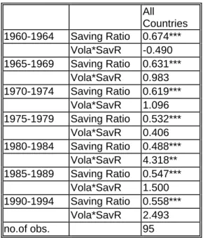
five-year periods (panel estimation)22 All Countries 1960-1964 Saving Ratio 0.674*** Vola*SavR -0.490 1965-1969 Saving Ratio 0.631*** Vola*SavR 0.983 1970-1974 Saving Ratio 0.619*** Vola*SavR 1.096 1975-1979 Saving Ratio 0.532*** Vola*SavR 0.406 1980-1984 Saving Ratio 0.488*** Vola*SavR 4.318** 1985-1989 Saving Ratio 0.547*** Vola*SavR 1.500 1990-1994 Saving Ratio 0.558*** Vola*SavR 2.493 no.of obs. 95

*/**/***: indicating that the coefficient is

significant at the 10/5/1 percent level.

Table 8: Saving retention coefficients for ten-year periods (panel estimation)23

All Countries 1960-1969 Saving Ratio 0.653*** Vola*SavR 0.799 1970-1979 Saving Ratio 0.550*** Vola*SavR 1.259 1980-1989 Saving Ratio 0.506*** Vola*SavR 3.662*** 1990-1996 Saving Ratio 0.545*** Vola*SavR 2.406* no. of obs. 190 (131)

*/**/***: indicating that the coefficient is

significant at the 10/5/1 percent level.

Number of observations for time period 90 to 96 given in brackets.

In the five- as well as in the ten-year period panel estimations the expected positive sign of the volatility interaction term can be found in the estimations (with the early sixties the only exception). This effect is statistically significant in the ten-year-panel for the 1980s and 7-year-panel for the 1990s. This supports the view that exchange rate volatility is among the factors relevant for both the low degree and the fluctuations of capital mobility. While in the

22

Detailed results can be found in Appendix II Table A9.

23

1960s and in part of the 1970s the Bretton Woods system was established and only gradual exchange rate changes took place, the 1980s have been marked by different periods of ex-change rate stability and therefore of exex-change rate sensitivity. Particularly the decreasing capital mobility in the first half of the 1990s in the EU could partly be caused by the increas-ing volatility of exchange rates in this period resultincreas-ing in a stronger current account targetincreas-ing. This finding backs the optimism that capital mobility will further increase in Europe with the introduction of the Euro.

The results for tax differentials are less conclusive. The basic idea about tax differentials af-fecting capital mobility is the following: If company taxes vary strongly in different countries, investment is more attractive in those countries with lower tax burdens.24 Increasing tax har-monization might reduce international mobility of capital insofar this mobility has been moti-vated by company’s reactions to tax differentials.

In order to catch the possible effect of differential company taxation on capital mobility, a measure of differential tax burden is constructed. This measure refers to direct business taxes according to the Fiscal Positions and Business Cycles of the OECD. In this data base Iceland, Turkey and Switzerland are not included, therefore the estimations presented below are based only on 20 countries.

As a rough macroeconomic proxy for the relative company tax burden the level of direct business taxes is set in relation to GDP. Since tax differentials are the focus of the analysis, direct business taxes/GDP of each country are subtracted from the OECD average of direct business taxes/GDP (taxdiff in the equation below).

If this deviation of a country’s company tax burden from the OECD average tax burden was zero for all countries, company tax burdens would be totally harmonized according to this indicator. The absolute deviation from zero can be interpreted as a measure for tax differen-tiation. The absolute value is used since deviation from OECD average tax burdens can be expected to induce capital mobility for both the case of a burden above average and the case of a burden below average.

24

Of course, there are other financial burdens such as national insurance contributions which are of relevance as well but which are not included in this analysis.

Diagram 6: OECD average of Direct Business Taxes/GDP minus National Direct Business Taxes/GDP. -0.020 -0.015 -0.010 -0.005 0.000 0.005 0.010 70 75 80 85 90 95 DIFFBUST1AUS 0.002 0.004 0.006 0.008 0.010 0.012 70 75 80 85 90 95 DIFFBUST1AUT -0.006 -0.004 -0.002 0.000 0.002 0.004 0.006 0.008 70 75 80 85 90 95 DIFFBUST1BEL -0.020 -0.015 -0.010 -0.005 0.000 0.005 0.010 70 75 80 85 90 95 DIFFBUST1CAN 0.004 0.006 0.008 0.010 0.012 0.014 70 75 80 85 90 95 DIFFBUST1DNK -0.005 0.000 0.005 0.010 0.015 70 75 80 85 90 95 DIFFBUST1ESP 0.000 0.005 0.010 0.015 0.020 0.025 70 75 80 85 90 95 DIFFBUST1FIN -0.002 0.000 0.002 0.004 0.006 0.008 70 75 80 85 90 95 DIFFBUST1FRA -0.010 -0.005 0.000 0.005 0.010 0.015 70 75 80 85 90 95 DIFFBUST1GBR -0.03 -0.02 -0.01 0.00 0.01 70 75 80 85 90 95 DIFFBUST1GER -0.005 0.000 0.005 0.010 0.015 0.020 70 75 80 85 90 95 DIFFBUST1GRC -0.005 0.000 0.005 0.010 0.015 0.020 70 75 80 85 90 95 DIFFBUST1IRE -0.005 0.000 0.005 0.010 0.015 0.020 70 75 80 85 90 95 DIFFBUST1ITA -0.035 -0.030 -0.025 -0.020 -0.015 -0.010 -0.005 70 75 80 85 90 95 DIFFBUST1JPN -0.012 -0.008 -0.004 0.000 0.004 70 75 80 85 90 95 DIFFBUST1NLD -0.06 -0.04 -0.02 0.00 0.02 70 75 80 85 90 95 DIFFBUST1NOR -0.05 -0.04 -0.03 -0.02 -0.01 0.00 70 75 80 85 90 95 DIFFBUST1NZL -0.005 0.000 0.005 0.010 0.015 0.020 70 75 80 85 90 95 DIFFBUST1PRT -0.005 0.000 0.005 0.010 0.015 0.020 70 75 80 85 90 95 DIFFBUST1SWE -0.015 -0.010 -0.005 0.000 0.005 0.010 70 75 80 85 90 95 DIFFBUST1USA

Note: A negative (positive) value of the tax differential variable refers to a country-specific tax burden which is above (below) average. Data source: OECD National Accounts, OECD Fiscal Positions and Business Cycles, own calculation.

Since differential company taxation should have an influence on private investment decision and not on government investment behavior, estimations were conducted on the basis of pri-vate sector data. The variable is included in the FH equation in the same way as the exchange rate volatility variable above:

(I/Y)it = α + (β0 + β1*| taxdiff it |)*(S/Y)it = α + β0 (S/Y)it + β1(| taxdiff |*S/Y) it with i the country index and t the time index.

A negative β1 would be in line with the hypothesis about large tax differentials to increase capital mobility. Tables 9 and 10 summarize the results of the panel estimations based on five- and ten-year periods. The tax-differential interaction with the saving ratio has both negative and positive signs in different periods. Only for the some cases with positive signs this variable is significant. Therefore the empirical results seem to indicate a decreasing effect of tax differentials on capital mobility. Obviously, these results should be interpreted very carefully since the chosen indicator measuring tax differentials might be too highly

aggre-gated. Further, the estimation method might be inadequate as the “autonomous” saving reten-tion coefficient generally looses its significance when introducing the volatility interacreten-tion term in the regression.

Apart from this, taxation is only one of a whole range of relevant variables relevant for the profitability of foreign direct investment. As direct investment is a long term decision, it can not easily be modified in the short run when changes in taxation take place. Insufficient tax harmonization might therefore rather have an impact on foreign portfolio investment being more flexible in the short or middle term.

Table 9: Saving retention coefficients for five-year periods (panel estimation, private sector)25

Core EU All countries 1971-1974 Saving Ratio -1.585 0.619*** Tax-Diff*SavR -8.709 (12) 6.912** (32) 1975-1979 Saving Ratio 0.5143** 0.286** Tax-Diff*SavR -2.337 (22) 1.967 (51) 1980-1984 Saving Ratio -0.094 0.140 Tax-Diff*SavR 8.872* (25) 7.057*** (70) 1985-1989 Saving Ratio 0.072 -0.098 Tax-Diff*SavR 10.931** (26) 7.719*** (71) 1990-1994 Saving Ratio 0.339** 0.143 Tax-Diff*SavR -4.558 (30) 9.134*** (75)

*/**/***: indicating that the coefficient is significant at the 10/5/1 percent level.

Number of observations is given in brackets.

Table 10: Saving retention coefficients for ten-year periods (panel estimation, private sector)26

Core EU All countries 1971-1979 Saving Ratio 0.374 0.472*** Tax-Diff*SavR -0.306 (34) 2.961 (83) 1980-1989 Saving Ratio 0.033 -0.005 Tax-Diff*SavR 10.157***(51) 7.466*** (141) 1990-1996 Saving Ratio 0.339** 0.136 Tax-Diff*SavR 0.282 (35) 9.000*** (87)

*/**/***: indicating that the coefficient is significant at the 10/5/1 percent level.

Number of observations is given in brackets.

25

Detailed results can be found in Appendix II Table A11.

26

VI. Conclusion

By definition EMU will increase capital mobility in the sense of equalizing nominal interest rates. The end of the nominal exchange rate risk eliminates exchange rate expectations and a possible exchange rate risk premium as determinants for interest rate differentials. In contrast to interest rate parity related concepts, the FH definition of capital mobility is not directly affected by the introduction of a single currency. However, the question how closely domestic saving and investment are tied together within EMU is important from a stabilization point of view. If the link is very strong, any shock affecting domestic saving capacity immediately influences domestic investment. Therefore, after the loss of the adjustment instrument of a nominal exchange rate, an increasing capital mobility in the FH sense would be particularly desirable.

In order to draw indirect conclusions for capital mobility within EMU the role of current ac-count targeting, exchange rate volatility and tax differentials have been explored in this paper. All three variables probably are affected by EMU. Current accounts will largely lose the character of a political target for national policy-makers. Exchange rate volatility is elimi-nated within the Eurozone. Finally, tax differentials can be expected to narrow due to intensi-fied tax competition under a single currency.

Behind this background two central results feed the expectation of increasing capital mobility in the FH sense within EMU: Current account targeting seems to have been one reason for low capital mobility. This conclusion can be drawn from the different results of the FH esti-mation approach for total saving and investment ratios on the one hand and for private sector aggregates on the other hand. Furthermore, there is some evidence that exchange rate volatil-ity had a limiting impact on capital mobilvolatil-ity. In particular, exchange rate volatilvolatil-ity is helpful to explain the decreasing capital mobility from the 1980s to the 1990s in Europe: This seems at least partly to have been caused by increasing capital account targeting. In contrast to these results the analysis of the impact of tax differentials is inconclusive.

The basic message is the following: After the introduction of the Euro the link between do-mestic saving and investment will be weakened for EMU member countries. This structural change is good news for the stabilization problem in a monetary union.

VII. References

ARTIS, M.J. AND T.A. BAYOUMI (1991): Global Capital Market Integration and the Current

Account, in: Mark P. Taylor (ed.): Money and Financial Markets, Cambridge.

BAYOUMI, T.A. (1990): Saving-Investment Correlations: Immobile Capital, Government

Policy, or Endogenous Behavior?, IMF Staff Papers 37(2), 360-387.

BHANDARI, JAGDEEP S. AND THOMAS H. MAYER (1990): A Note on Saving-Investment

Cor-relation in the EMS, IMF Working Paper, No. WP/90/97, Washington.

DORNBUSCH, RUDIGER (1991): Comment on Feldstein/Bacchetta, in: B. Douglas Bernheim (ed): Saving and Economic Performance, Univ. of Chicago Press, 220-226.

FELDSTEIN, MARTIN AND PHILIPPE BACCHETTA (1991): National Saving and International

Investment, in: B. Douglas Bernheim (ed): Saving and Economic Performance, Univ. of Chi-cago Press, 201-226.

FELDSTEIN, MARTIN UND CHARLES HORIOKA (1980): Domestic Saving and International Capital Flows, The Economic Journal, 90, 314-329.

HELLIWELL, JOHN F. AND ROSS MCKITRICK (1998): Comparing Capital Mobility Across

Pro-vincial and National Borders, NBER Working Paper 6624, Cambridge.

HOGENDORN, CHRISTIAAN (1998): Capital Mobility in Historical Perspective, Journal of

Pol-icy Modeling, 20(2), 141-161.

INGRAM, JAMES C. (1959): State and Regional Payments Mechanisms, Quarterly Journal of

Economics, 73, 619-632.

LEMMEN, JAN J. G. AND SYLVESTER C. W. EIJFFINGER (1995): The Quantity Approach to

Fi-nancial Integration: The Feldstein-Horioka Criterion Revisited, Open Economies Review 6, 145-165.

OECD (1998): National Accounts, Vol. I and II.

SINN, STEFAN (1992): Saving-Investment Correlations and Capital Mobility: On the Evidence

from Annual Data, The Economic Journal, 102, 1162-1170.

SUMMERS, LARRY H, (1988): Tax Policy and International Competitiveness, in: J.A. Frankel

(ed): International Aspects of Fiscal Policies, Chicago, The University of Chicago Press, 350-380.

VAMVAKIDIS, ATHANASIOS AND ROMAIN WACZIARG (1998): Developing Countries and the

APPENDIX I:

Illustration 1: Gross investment ratio(broken line) and gross saving ratio (thin line)

0.14 0.16 0.18 0.20 0.22 0.24 0.26 0.28 60 65 70 75 80 85 90 95 INVRAUS SAVRAUS 0.20 0.22 0.24 0.26 0.28 0.30 0.32 60 65 70 75 80 85 90 95 INVRAUT SAVRAUT 0.12 0.14 0.16 0.18 0.20 0.22 0.24 0.26 0.28 60 65 70 75 80 85 90 95 INVRBEL SAVRBEL 0.12 0.14 0.16 0.18 0.20 0.22 0.24 0.26 60 65 70 75 80 85 90 95 INVRCAN SAVRCAN 0.10 0.12 0.14 0.16 0.18 0.20 0.22 0.24 0.26 60 65 70 75 80 85 90 95 INVRDNK SAVRDNK 0.18 0.20 0.22 0.24 0.26 0.28 0.30 60 65 70 75 80 85 90 95 INVRESP SAVRESP 0.10 0.15 0.20 0.25 0.30 0.35 60 65 70 75 80 85 90 95 INVRFIN SAVRFIN 0.16 0.18 0.20 0.22 0.24 0.26 0.28 60 65 70 75 80 85 90 95 INVRFRA SAVRFRA 0.12 0.14 0.16 0.18 0.20 0.22 60 65 70 75 80 85 90 95 INVRGBR SAVRGBR 0.18 0.20 0.22 0.24 0.26 0.28 0.30 60 65 70 75 80 85 90 95 INVRGER SAVRGER 0.10 0.15 0.20 0.25 0.30 0.35 0.40 0.45 60 65 70 75 80 85 90 95 INVRGRC SAVRGRC 0.10 0.15 0.20 0.25 0.30 0.35 60 65 70 75 80 85 90 95 INVRICE SAVRICE

0.10 0.15 0.20 0.25 0.30 60 65 70 75 80 85 90 95 INVRIRE SAVRIRE 0.16 0.20 0.24 0.28 0.32 60 65 70 75 80 85 90 95 INVRITA SAVRITA 0.26 0.28 0.30 0.32 0.34 0.36 0.38 0.40 0.42 60 65 70 75 80 85 90 95 INVRJPN SAVRJPN 0.1 0.2 0.3 0.4 0.5 0.6 60 65 70 75 80 85 90 95 INVRLUX SAVRLUX 0.18 0.20 0.22 0.24 0.26 0.28 0.30 0.32 60 65 70 75 80 85 90 95 INVRNLD SAVRNLD 0.15 0.20 0.25 0.30 0.35 0.40 60 65 70 75 80 85 90 95 INVRNOR SAVRNOR 0.12 0.16 0.20 0.24 0.28 0.32 60 65 70 75 80 85 90 95 INVRNZL SAVRNZL 0.10 0.15 0.20 0.25 0.30 0.35 0.40 60 65 70 75 80 85 90 95 INVRPRT SAVRPRT 0.10 0.12 0.14 0.16 0.18 0.20 0.22 0.24 0.26 60 65 70 75 80 85 90 95 INVRSWE SAVRSWE 0.20 0.22 0.24 0.26 0.28 0.30 0.32 0.34 0.36 60 65 70 75 80 85 90 95 INVRSWI SAVRSWI 0.10 0.15 0.20 0.25 0.30 60 65 70 75 80 85 90 95 INVRTRK SAVRTRK 0.12 0.14 0.16 0.18 0.20 0.22 60 65 70 75 80 85 90 95 INVRUSA SAVRUSA

Illustration 2: Gross saving ratios (bold line), gross private saving ratios (thin line) and gross private fixed capital investment ratios (broken line)

0.14 0.16 0.18 0.20 0.22 0.24 0.26 0.28 60 65 70 75 80 85 90 95

GSAVAUS GPRSAVAUS GPRFCFAUS

0.18 0.20 0.22 0.24 0.26 0.28 0.30 0.32 60 65 70 75 80 85 90 95

GSAVAUT GPRSAVAUT GPRFCFAUT

0.12 0.14 0.16 0.18 0.20 0.22 0.24 0.26 0.28 60 65 70 75 80 85 90 95

GSAVBEL GPRSAVBEL GPRFCFBEL

0.12 0.14 0.16 0.18 0.20 0.22 0.24 0.26 60 65 70 75 80 85 90 95

GSAVCAN GPRSAVCAN GPRFCFCAN

0.08 0.12 0.16 0.20 0.24 0.28 60 65 70 75 80 85 90 95 GSAVDRK GPRSAVDRK GPRFCFDRK 0.10 0.15 0.20 0.25 0.30 0.35 60 65 70 75 80 85 90 95

GSAVFIN GPRSAVFIN GPRFCFFIN

0.14 0.16 0.18 0.20 0.22 0.24 0.26 0.28 60 65 70 75 80 85 90 95

GSAVFRA GPRSAVFRA GPRFCFFRA

0.16 0.18 0.20 0.22 0.24 0.26 0.28 0.30 60 65 70 75 80 85 90 95

GSAVGER GPRSAVGER GPRFCFGER

0.10 0.15 0.20 0.25 0.30 0.35 60 65 70 75 80 85 90 95

GSAVITA GPRSAVITA GPRFCFITA

0.20 0.25 0.30 0.35 0.40 0.45 60 65 70 75 80 85 90 95 GSAVJPN GPRSAVJPN GPRFCFJPN 0.12 0.16 0.20 0.24 0.28 0.32 60 65 70 75 80 85 90 95 GSAVNLD GPRSAVNLD GPRFCFNLD 0.15 0.20 0.25 0.30 0.35 60 65 70 75 80 85 90 95

GSAVNOR GPRSAVNOR GPRFCFNOR

0.08 0.12 0.16 0.20 0.24 0.28 60 65 70 75 80 85 90 95

GSAVSWE GPRSAVSWE GPRFCFSWE

0.10 0.12 0.14 0.16 0.18 0.20 0.22 60 65 70 75 80 85 90 95

GSAVUK GPRSAVUK GPRFCFUK

0.12 0.14 0.16 0.18 0.20 0.22 0.24 60 65 70 75 80 85 90 95

APPENDIX II

Table A1: Saving retention coefficients for cross section estimations for each single year for gross total

invest-ment and saving data year Core countries All Countries 1960 0.512 (5.758) 0.594 (5.184) 1961 0.541 (4.554) 0.579 (6.462) 1962 0.502 (2.274) 0.751 (9.571) 1963 0.698 (5.605) 0.835 (10.358) 1964 0.567 (2.071) 0.809 (11.604) 1965 0.704 (3.153) 0.691 (8.005) 1966 0.454 (2.089) 0.675 (7.099) 1967 0.366 (1.233) 0.662 (6.063) 1968 0.556 (1.494) 0.591 (4.788) 1969 0.098 (0.296) 0.645 (7.031) 1970 -0.039 (-0.171) 0.587 (7.894) 1971 0.309 (1.163) 0.707 (9.365) 1972 0.751 (2.445) 0.700 (10.072) 1973 0.467 (1.730) 0.713 (9.253) 1974 0.332 (1.110) 0.530 (4.205) 1975 0.590 (2.941) 0.487 (2.823) 1976 0.107 (0.256) 0.480 (2.835) 1977 0.433 (1.427) 0.530 (2.809) 1978 0.208 (1.576) 0.599 (4.623) 1979 0.255 (5.589) 0.580 (4.744) 1980 0.439 (7.852) 0.550 (5.882) 1981 0.581 (4.795) 0.507 (3.457) 1982 0.438 (3.633) 0.558 (3.438) 1983 0.507 (3.857) 0.639 (4.393) 1984 0.432 (3.633) 0.446 (4.058) 1985 0.353 0.337

(2.513) (3.148) 1986 0.273 (1.146) 0.503 (4.738) 1987 0.375 (1.579) 0.588 (6.529) 1988 0.441 (2.067) 0.639 (7.459) 1989 0.352 (1.886) 0.535 (6.090) 1990 0.466 (2.399) 0.512 (5.484) 1991 0.733 (3.187) 0.512 (5.179) 1992 0.907 (3.151) 0.529 (5.801) 1993 0.736 (2.028) 0.559 (4.826) 1994 0.664 (1.804) 0.612 (4.768) 1995 0.571 (1.051) 0.561 (4.024) 1996 0.326 (2.958) 0.493 (3.570) no. of obs. _{6 23} (t-values in brackets)

Table A2: Regression results using five-year averages of total investment and saving ratios time period variable Core Countries Rest of EU Rest of the World All Countries 1960-1964 Constant 0.061 (1.605) 0.068 (1.412) 0.045 (2.342) 0.057 (3.194) Saving Ratio 0.688 (4.696) 0.711 (3.361) 0.794 (10.645) 0.737 (10.147) R² adjusted 0.808 0.595 0.934 0.823 no. Of observ. 6 8 9 23 1965-1969 Constant 0.089 (1.216) 0.078 (1.576) 0.069 (1.983) 0.074 (3.376) Saving Ratio 0.606 (2.140) 0.665 (3.240) 0.689 (5.155) 0.674 (7.834) R² adjusted 0.417 0.576 0.762 0.733 no. Of observ. 6 8 9 23 1970-1974 Constant 0.094 (1.251) 0.090 (3.511) 0.057 (1.670) 0.070 (3.653) Saving Ratio 0.576 (2.060) 0.619 (6.463) 0.739 (5.992) 0.685 (9.685) R² adjusted 0.394 0.853 0.814 0.808 no. Of observ. 6 8 9 23 1975-1979 Constant 0.104 (1.663) 0.142 (2.365) 0.090 (1.433) 0.105 (2.996) Saving Ratio 0.538 (1.932) 0.456 (1.748) 0.673 (2.600) 0.594 (3.968) R² adjusted 0.354 0.227 0.419 0.401 no. Of observ. 6 8 9 23 1980-1984 Constant 0.091 (3.641) 0.099 (1.131) 0.120 (3.802) 0.105 (3.761) Saving Ratio 0.564 (40441) 0.662 (4.024) 0.503 (3.703) 0.572 (4.394)

R² adjusted 0.789 0.169 0.614 0.454 no. Of observ. 6 8 9 23 1985-1989 Constant 0.116 (2.411) 0.067 (1.837) 0.127 (6.492) 0.103 (5.589) Saving Ratio 0.398 (1.756) 0.730 (4.024) 0.474 (5.661) 0.539 (6.353) R² adjusted 0.294 0.685 0.795 0.641 no. Of observ. 6 8 9 23 1990-1994 Constant 0.020 (0.270) 0.096 (2.044) 0.100 (3.737) 0.091 (4.557) Saving Ratio 0.831 (2.362) 0.572 (3.161) 0.547 (4.418) 0.562 (5.777) R² adjusted 0.478 0.562 0.698 0.595 no. Of observ. 6 8 9 23 (t-values in brackets)

Table A3: Regression results using ten-year averages of total investment and saving ratios time variable Core Countries Rest of EU Rest of World All Countries 1960-1969 Constant 0.068 (1.464) 0.055 (1.368) 0.064 (2.608) 0.065 (3.962) Saving Ratio 0.673 (3.724) 0.766 (4.477) 0.716 (7.483) 0.708 (10.756) R² adjusted 0.720 0.731 0.873 0.839 no. of observ. 6 8 9 23 1970-1979 Constant 0.097 (1.600) 0.091 (2.421) 0.080 (2.331) 0.082 (3.833) Saving Ratio 0.560 (2.236) 0.646 (4.279) 0.683 (5.110) 0.666 (7.819) R² adjusted 0.445 0.712 0.758 0.732 no. of observ. 6 8 9 23 1980-1989 Constant 0.098 (3.086) 0.045 (0.854) 0.134 (5.656) 0.104 (4.949) Saving Ratio 0.505 (3.247) 0.886 (3.411) 0.439 (4.284) 0.553 (5.638) R² adjusted 0.656 0.603 0.684 0.583 no. of observ. 6 8 9 23 1990-1999 Constant 0.033 (0.394) 0.061 (2.608) 0.110 (3.648) 0.094 (4.152) Saving Ratio 0.765 (1.972) 0.707 (2.132) 0.497 (3.550) 0.532 (4.834) R² adjusted 0.366 0.336 0.592 0.504 no. of observ. 6 8 9 23 (t-values in brackets)

Table A4: Regression results for five-year periods for total investment and saving ratios (panel estimation)

time period variable Core Countries Rest of EU Rest of World All Countries 1960-1964 Constant 0.097 (4.886) 0.088 (4.238) 0.046 (3.766) 0.067 (6.740) Saving Ratio 0.534 (6.936) 0.624 (6.901) 0.792 (16.420) 0.696 (17.335) R² adjusted 0.619 0.545 0.859 0.724 no. Of observ. 30 40 45 115 1965-1969 Constant 0.136 (4.144) 0.087 (3.755) 0.075 (4.343) 0.081 (7.049) Saving Ratio 0.413 (3.253) 0.628 (6.554) 0.673 (10.281) 0.644 (17.267) R² adjusted 0.248 0.518 0.704 0.640 no. Of observ. 30 40 45 115 1970-1974 Constant 0.157 (5.064) 0.108 (7.182) 0.058 (3.603) 0.081 (7.761) Saving Ratio 0.327 (2.832) 0.552 (9.886) 0.739 (12.665) 0.642 (16.670) R² adjusted 0.195 0.713 0.784 0.708 no. Of observ. 30 40 45 115 1975-1979 Constant 0.152 (7.872) 0.158 (6.342) 0.092 (3.368) 0.119 (7.379) Saving Ratio 0.315 (3.586) 0.384 (3.562) 0.669 (5.966) 0.533 (7.770) R² adjusted 0.290 0.231 0.440 0.342 no. Of observ. 30 40 45 115 1980-1984 Constant 0.099 (8.311) 0.130 (4.250) 0.117 (8.924) 0.111 (9.004) Saving Ratio 0.510 (8.417) 0.509 (3.459) 0.524 (9.396) 0.544 (9.557) R² adjusted 0.707 0.219 0.665 0.442 no. Of observ. 30 40 45 115 1985-1989 Constant 0.121 (7.721) 0.077 (4.190) 0.130 (11.865) 0.107 (11.619) Saving Ratio 0.364 (4.922) 0.682 (7.490) 0.463 (9.912) 0.520 (12.324) R² adjusted 0.445 0.586 0.688 0.570 no. Of observ. 30 40 45 115 1990-1994 Constant 0.045 (1.877) 0.053 (2.300) 0.103 (8.319) 0.091 (9.359) Saving Ratio 0.706 (6.339) 0.788 (6.233) 0.530 (9.298) 0.558 (11.794) R² adjusted 0.575 0.492 0.660 0.548 no. Of observ. 30 40 45 115 (t-values in brackets)

Table A5: Regression results for five-year periods based on cyclically adjusted data for total investment and saving ratios (panel estimation)

time period variable Core Countries Rest of EU Rest of the World All countries 1960-1964 Constant 0.089 (5.289) 0.077 (3.753) 0.047 (5.623) 0.063 (7.356)) Saving Ratio Trend 0.566 (8.696) 0.674 (7.556) 0.789 (24.026) 0.710 (20.358) R² adjusted 0.720 0.590 0.929 0.784 no. of observ. 30 40 45 115 1965-1969 Constant 0.145 (5.341) 0.079 (4.900) 0.057 (4.591) 0.066 (7.744) Saving Ratio Trend 0.383 (3.688) 0.658 10.059 0.742 (15.782) 0.701 (21.011) R² adjusted 0.303 0.720 0.849 0.794 no. of observ. 30 40 45 115 1970-1974 Constant 0.151 (6.443) 0.086 (6.692) 0.059 (4.160) 0.071 (7.671) Saving Ratio Trend 0.347 (3.889) 0.646 (13.077) 0.746 (14.261) 0.690 (19.831) R² adjusted 0.327 0.813 0.821 0.775 no. of observ. 30 40 45 115 1975-1979 Constant 0.128 (9.790) 0.130 (5.718) 0.075 (3.946) 0.096 (7.477) Saving Ratio Trend 0.418 (7.256) 0.511 (5.264) 0.729 (9.500) 0.627 (11.622) R² adjusted 0.642 0.407 0.669 0.540 no. of observ. 30 40 45 115 1980-1984 Constant 0.110 (13.610) 0.096 (3.081) 0.118 (9.682) 0.102 (8.845) Saving Ratio Trend 0.452 (11.117) 0.656 (4.371) 0.523 (10.035) 0.579 (10.800) R² adjusted 0.808 0.317 0.694 0.504 no. of observ. 30 40 45 115 1985-1989 Constant 0.112 (9.377) 0.060 (3.283) 0.121 (16.248) 0.103 (12.635) Saving Ratio Trend 0.407 (7.178) 0.786 (8.531) 0.496 (15.316) 0.543 (14.363) R² adjusted 0.635 0.648 0.841 0.643 no. of observ. 30 40 45 115 1990-1994 Constant 0.053 (2.269) 0.048 (2.133) 0.098 (9.176) 0.088 (9.921) Saving Ratio Trend 0.667 (6.160) 0.801 (6.604) 0.550 (11.230) 0.570 (13.362) R² adjusted 0.560 0.522 0.740 0.609 no. of observ. 30 40 45 115 (t-values in brackets)

Table A6: Regression results for ten-year periods for total investment and saving ratios (panel estimation)

time period variable Core Countries Rest of EU Rest of World All Countries 1960-1969 Constant 0.110 (6.000) 0.088 (5.851) 0.060 (5.747) 0.073 (9.735) Saving Ratio 0.499 (7.028) 0.625 (9.856) 0.732 (18.001) 0.674 (22.581) R² adjusted 0.451 0.549 0.784 0.690 no. Of observ. 60 80 90 230 1970-1979 Constant 0.131 (9.797) 0.138 (9.907) 0.082 (5.520) 0.106 (11.843) Saving Ratio 0.413 (7.635) 0.455 (8.230) 0.679 (11.907) 0.527 (15.935) R² adjusted 0.493 0.458 0.613 0.525 no. Of observ. 60 80 90 230 1980-1989 Constant 0.111 (11.436) 0.105 (5.467) 0.124 (14.814) 0.109 (14.006) Saving Ratio 0.428 (8.998) 0.587 (6.253) 0.490 (13.708) 0.530 (14.751) R² adjusted 0.575 0.325 0.677 0.486 no. Of observ. 60 80 90 230 1990-1996 Constant 0.056 (2.449) 0.063 (5.625) 0.102 (8.735) 0.089 (9.550) Saving Ratio 0.645 (6.118) 0.699 (5.625) 0.527 (9.783) 0.550 (12.123) R² adjusted 0.489 0.380 0.637 0.503 no. Of observ. 39 51 55 145 (t-values in brackets)

Table A7: Regression results for five-year periods for private sector data

PERIOD-AVERAGED DATA

PANEL ESTIMATION

Time period variable All countires Core EU All countries 1970-1974 Constant 0.081 (1.935) 0.213 (9.109) 0.079 (4.395) Gross Private Saving 0.624

(3.159) -0.059 (-0.531) 0.327 (7.472) R² adjusted 0.529 -0.042 0.560 no. of observ. 9 19 44 1975-1979 Constant 0.121 (2.893) 0.141 (6.844) 0.131 (6.984) Gross Private Saving 0.383

(1.916) 0.232 (2.295) 0.336 (3.707) R² adjusted 0.229 0.157 0.188 no. of observ. 10 24 56 1980-1984 Constant 0.108 (2.554) 0.111 (2.859) 0.112 (5.870) Gross Private Saving 0.366

(1.816) 0.288 (1.478) 0.346 (3.813) R² adjusted 0.141 0.039 0.155 no. of observ. 15 30 75 1985-1989 Constant 0.177 0.161 0.182

(5.276) (9.422) (12.189) Gross Private Saving 0.046

(0.281) 0.059 (0.717) 0.021 (0.287) R² adjusted -0.070 -0.017 -0.013 no. of observ. 15 30 75 1990-1994 Constant 0.078 (0.283) 0.098 (2.915) 0.117 (5.902) Gross Private Saving 0.455

(2.497) 0.342 (2.250) 0.264 (2.741) R² adjusted 0.272 0.123 0.081 no. of observ. 15 30 75 (t-values in brackets)

Table A8: Regression results for ten-year periods for private sector data

PERIOD-AVERAGED DATA

PANEL ESTIMATION

time period variable Core Countries Core Countries All Countries 1970-1979 Constant 0.097 (2.228) 0.173 (10.500) 0.100 (7.572) Gross Private Saving 0.523 (2.529) 0.098 (1.233) 0.504 (8.005) R² adjusted 0.403 0.011 0.389 no. of observ. 9 46 100 1980-1989 Constant 0.145 (3.817) 0.147 (8.671) 0.155 (12.915) Gross Private Saving 0.196 (1.061) 0.118 (1.417) 0.147 (2.536) R² adjusted 0.009 0.017 0.0352 no. of observ. 15 60 150 1990-1995 Constant 0.073 (1.898) 0.098 (3.046) 0.119 (6.267) Gross Private Saving 0.471 (2.540) 0.339 (2.344) 0.248 (2.731) R² adjusted 0.280 0.117 0.070 no. of observ. 15 35 87 (t-values in brackets)

Table A9: Regression results for five-year periods for total saving and investment ratios including the Vola*Saving ratio interaction (panel estimation) time period variable All Countries t-statistics R² adjusted no. of observ. 1960-1964 Constant 0.071 6.182 0.696 95 Saving Ratio 0.674 14.404 Saving Ratio*Vola -0.490 -0.119 1965-1969 Constant 0.081 7.207 0.697 95 Saving Ratio 0.631 14.683 Saving Ratio*Vola 0.983 0.895 1970-1974 Constant 0.083 8.400 0.780 95 Saving Ratio 0.619 16.350 Saving Ratio*Vola 1.096 1.150 1975-1979 Constant 0.115 6.352 0.336 95 Saving Ratio 0.532 6.619 Saving Ratio*Vola 0.406 0.222 1980-1984 Constant 0.109 8.114 0.476 95 Saving Ratio 0.488 7.323 Saving Ratio*Vola 4.318 2.296 1985-1989 Constant 0.094 9.873 0.649 95 Saving Ratio 0.547 11.646 Saving Ratio*Vola 1.500 0.997 1990-1994 Constant 0.0821 8.214 0.624 95 Saving Ratio 0.558 10.873 Saving Ratio*Vola 2.493 1.534

Table A10: Regression results for ten-year periods for total saving and investment ratios including a Vola*Saving ratio interaction (panel estimation)

time period variable All Countries t-statistics R² adjusted no. of observ. 1960-1969 Constant 0.076 9.483 0.701 190 Saving Ratio 0.653 20.892 Saving Ratio*Vola 0.799 0.714 1970-1979 Constant 0.105 11.057 0.557 190 Saving Ratio 0.550 14.260 Saving Ratio*Vola 1.259 1.270 1980-1989 Constant 0.102 12.241 0.542 190 Saving Ratio 0.506 12.257 Saving Ratio*Vola 3.662 3.014 1990-1996 Constant 0.081 8.461 0.588 120 Saving Ratio 0.545 11.198 Saving Ratio*Vola 2.520 1.921

Table A11: Regression results for five-year periods for private saving ratio including a tax-differential saving

ra-tio interacra-tion (panel estimara-tion) GROSS PRIVATE DATA

time period variable Core Coun-tries All Countries 1971-1974 constant 0.569 (2.156) 0.064 (2.774) Saving Ratio -1.585 (-1.404) 0.620 (5.354) Tax-Differential -8.709 (-1.167) 6.913 (2.063) adjusted R2 0.004 0.631 no. of obs. 12 32 1975-1979 constant 0.083 (1.634) 0.137 (5.842) Saving Ratio 0.514 (2.212) 0.286 (2.337) Tax-Differential -2.337 (-1.284) 1.967 (0.718) adjusted R2 0.295 0.145 no. of obs. 22 51 1980-1984 constant 0.183 (2.868) 0.142 (7.937) Saving Ratio -0.094 (-0.312) 0.140 81.597) Tax-Differential 8.872 (2.071) 7.057 (4.868) adjusted R2 0.130 0.323 no. of obs. 25 70 1985-1989 constant 0.144 (5.128) 0.194 (13.453) Saving Ratio 0.072 (0.546) -0.098 8-1.367) Tax-Differential 10.931 (2.663) 7.716 (5.199) adjusted R2 0.208 0.264 no. of obs. 26 71 1990-1994 constant 0.104 (2.963) 0.128 (7.057) Saving Ratio 0.339 (2.206) 0.143 (1.562) Tax-Differential -4.559 (-0.674) 9.134 (4.205) adjusted R2 0.105 0.252 no. of obs. 30 75 (t-values in brackets)

Table A12: Regression results for ten-year periods for pri-vate saving ratio including a tax-differential saving ratio

interaction (panel estimation) GROSS PRIVATE DATA

time period variable Core Coun-tries All Countries 1971-1979 constant 0.112 (1.925) 0.099 (5.747) Saving Ratio 0.374 (1.439) 0.473 (5.364) Tax-Differential -0.306 (-0.151) 2.961 (1.344) adjusted R2 0.038 0.364 no. of obs. 34 83 1980-1989 constant 0.154 (6.122) 0.174 (15.364) Saving Ratio 0.033 (0.283) -0.005 (0.093) Tax-Differential 10.157 (3.708) 7.466 (7.186) adjusted R2 0.224 0.278 no. of obs. 51 141 1990-1995 constant 0.098 (2.888) 0.128 (7.334) Saving Ratio 0.339 (2.309) 0.136 (1.563) Tax-Differential 0.282 (0.045) 9.000 (4.261) adjusted R2 0.089 0.226 no. of obs. 35 87 (t-values in brackets)