Development of a Semi-definite Programming
Weighted Sum Based Approach for Solving
Stochastic Multi-objective Economic Dispatch
Problems Incorporating CHP Units
Kolapo Alli, Member, IAENG, A.M Jubril, and L.O Kehinde
Abstract—This paper has presented a weighted sum based semidefinite programming (SDP) optimization technique for solving stochastic multi-objective economic dispatch (MOED) model that incorporates Combined Heat and Power (CHP) units. The stochastic multi-objective model was transformed into its deterministic equivalent through their expectation, with the assumption that involved random variables are normally distributed. The multi-objective problem was recast in matrix form as a SDP relaxation problem and subsequently solved with a MATLAB programming suite. The system inequality and equality constraints uncertainty were entered into YALMIP, which is a linear matrix inequality parser. Simulations were performed on modified IEEE 6 and 20 units’ networks with 2 CHP units. The efficiency of the proposed method is deter-mined by investigating reformulated problems in stochastic and deterministic models on power dispatch. The standard weighted sum method is utilized in generating the Pareto-optimal solution between two objectives’ functions. An optimal selection of control weight selection k1 parameter that provides a better convergence property and moderately good extent of the Pareto distributions was empirically determined. The proposed SDP method performed well in accuracy of results and providing lower operational cost in the Pareto set produced.
Index Terms—SDP, stochastic Multi-objectives problem, Pareto Distribution.
I. INTRODUCTION
T
HE reduction of operational cost of power production in electrical power system analysis can be simply re-ferred to as economic dispatch (ED) [1]. Thus, the problem in economic dispatch becomes multi-objective optimization when two or more objectives’ functions are considered in the optimization model such as the total running fuel cost and the total emission are to be minimized simultaneously by adjusting the output power of every single generator while meeting the load demand and satisfying the system’s constraints.However, in recent years, cogeneration unit popularly known as combined heat and power (CHP) unit has become an essential energy production technology in many countries due to its advanced efficiency in the production of total
Manuscript received May 11, 2016; revised July 18, 2017.
Dr. K.S. Alli is with the Department of Electrical/Electronic and Com-puter Engineering, Afe Babalola University, Ado-Ekiti, Nigeria. Email: [email protected]
Dr. A.M. Jubril is with the Department of Electronic and Electri-cal Engineering, Obafemi Awolowo University, Ile-Ife, Nigeria. Email: [email protected]
Prof. L.O. Kehinde is with the Department of Electronic and Electrical Engineering, Obafemi Awolowo University, Ile-Ife, Nigeria. Email: [email protected]
energy which can produce sufficient different heat and power generation. Moreso, the heat generated by CHP units can be used for heating or industrial purposes. It is more important to know that the load demand is unstable in nature [2]. There-fore, problems in CHP are usually formulated as stochastic model and based on this, different power dispatch plans can be modeled. The main objectives in CHP units dispatch are to ensure sufficient production of power and heat, and fuel costs minimization.
Some of the works that are relevant to this study are hereby presented. Particle Swarm Optimization method for solving Stochastic Multi-Objective Dispatch Problems has been reported in[2],[3],[4],[5],[6],[7],[8],[9],[10],[11]. A bi-objective economic dispatch model incorporating wind power units has been formulated in [12], whereby opera-tional cost and security effects are considered as conflicting objectives. Some evolutionary optimization methods based on stochastic searching techniques have been presented in [13],[14],[15],[16],[17],[18] to achieve optimal power flow problems resolutions. Problems such as smooth, non-smooth and piecewise fuel cost objectives were considered in the presented works.
Quasi-oppositional teaching learning based optimization (QOTLBO) has been proposed by [19] to solve non-linear multi-objective economic emission dispatch (EED) formu-lated problem of electric power generation with valve point loading. Also, recent studies on optimal power flow prob-lems have been solved by the hybridization of stochastic searching-based optimization techniques proposed by [20], [21]. Similarly, a study on PID controller design for an au-tomatic generation control of multi-area power units network has been addressed in [22] using Firefly algorithm. A three level decomposition technique has been presented in [23] for solving problems on ac-unit commitment and a robust commitment schedule to resist the stochastic wind power generation. More so, a mixed integer linear programming has been proposed for solving multi-carrier power systems problems presented in [24].
An optimization approach based on generalized bender de-composition has been presented in [25] for solving volt-age problems in transmission and distribution networks of distributed generation units such as wind and solar power systems. Furthermore, a direct search optimization technique has been presented in [26] for the reduction of fuel cost taken into account the inter-area power flow and reserve capacity constraints.
Many techniques involved in handling the multi-objective
IAENG International Journal of Computer Science, 44:4, IJCS_44_4_10
CHP problem (both deterministic and stochastic) are all heuristic in nature [27]. These evolutionary methods are population based algorithms and can generate a number of solutions over several runs. However, because they are stochastic in nature, the attainment of the Pareto solutions are not guaranteed to converge to the ideal optimal solu-tion set: they involve multiple runs and different solusolu-tions obtained in each run which result to keeping the statistical data by obtaining the best and worst optimal solutions. Another problem about these evolutionary methods is their less capacity of dealing with problem constraints, which pro-duces non-feasible solutions. Examples of these algorithms are genetic algorithms (GAs), particle swarm optimization technique (PSO), they consumed much time in evaluating a large number of functions. On the other hand, semi-definite programming (SDP)-based weighted sum approach proposed in this paper is not a population based algorithm but convex optimization technique and have been shown to be useful in attaining the global optimal solution over several runs; therefore, the global optimality of its solution is assured, if the problem is convex. Likewise, for non-convex problem, semi-definite relaxation of the problem gives an estimated convex form that generates an approximation bound for the problem [27]. The applications of SDP to optimal power flow (OPF) and economic dispatch (ED) problems can be found in [27],[28],[29],[30],[31],[32],[33]. The paper is structured as follows: Section I presents the introduction and literature reviews, Section II describes the formulation of stochastic multi-objective problems, constraints and their SDP relaxation forms, Section III discusses the description of semi-definite programming approach. Section IV reports the simulations and results and Section V is the conclusion.
II. PROBLEMOBJECTIVES
A. Total cost function
The objective function for the Total cost(J1)is formulated
as [7] J1= Np X i=1 Ci(Pi) + Nc X j=1 Cj(Θj, Hj) + Nh X k=1 Ck(Tk) (1) where Np are the numbers of conventional power units, Nc are the numbers of electrical and thermal power outputs units and Nh are the numbers of heat units, respectively. The expected stochastic objective cost functionJ1is further
expressed as follows [7]: J1= Np X i=1 {αi+βiP¯i+γi( ¯Pi2+V ar(Pi))}+ Nc X j=1 {αj+ βjΘ¯j+γj( ¯Θj 2 +V ar(Θj)) +δjH¯j+ Θj( ¯Hj 2 + V ar(Hj)) +ξj( ¯ΘjH¯j+Cov(Θj, Hj)}+ Nh X k=1 {αk+ δkT¯k+θk( ¯Tk2+V ar(Tk))} (2) wherebyαi,βi,γi are the running cost coefficients of the ith thermal unit, Pi is the power output of the ith unit, Θj and Hj are the electrical and thermal power output coefficients of the jth chp unit respectively. Also, αj,βj, γj,δj,θj,ξj
are the cost coefficients of the jth chp unit andαi,δk,θk are the cost coefficients of the kth heat-only unit.
Where the terms V ar(Pi) = V2(Pi) ¯Pi
2 , V ar(Tk) = V2(Tk) ¯Tk 2 , Coυ(Θj, Hj) = C2(Θj, Hj) ¯Θj 2 ¯ Hj, and V(), C() are the variance coefficients and correlation
coeffi-cients of all the random variables respectively. The coefficient of variance of all the involved random variables is chosen as 0.2, and the correlation coefficient of each pair of random variables is set as 0.3 [7]. ¯ J1= Np X i=1 {αi+βiP¯i+γi( ¯Pi2+V 2(P i)) ¯Pi 2 }+ Nc X j=1 {αj+ βjΘ¯j+γj( ¯Θj 2 +V2(Θj) ¯Θj 2 ) +δjH¯j+θj( ¯Hj 2 + V2(Hj) ¯Hj 2 ) +ξj( ¯ΘjH¯j+C2(Θj, Hj) ¯ΘjH¯j}+ Nh X k=1 {αk+δkT¯k+θk( ¯Tk2+V 2(T k) ¯Tk 2 )} (3) ¯ J1= Np X i=1 {αi+βiP¯i+γi(1 +V2(Pi)) ¯Pi 2 }+ Nc X j=1 {αj+βjΘ¯j +γj(1 +V2(Θj)) ¯Θj 2 +δjH¯j+θj(1 +V2(Hj)) ¯Hj 2 +ξj(1 +C2(Θj, Hj)) ¯ΘjH¯j}+ Nh X k=1 {αk+δkT¯k+θk(1+ V2(Tk)) ¯Tk 2 } ¯ J1= Np X i=1 {αi+βiP¯i+γi(1 + 0.04) ¯Pi 2 }+ Nc X j=1 {αj+βjΘ¯j+ γj(1 + 0.04) ¯Θj 2 +δjH¯j+θj(1 + 0.04) ¯Hj 2 + ξj(1 + 0.09) ¯ΘjH¯j}+ Nh X k=1 {αk+δkT¯k+θk(1 + 0.04) ¯Tk 2 }
The conversion of Eq. (II-A) to its equivalent deterministic model becomes; ¯ J1= Np X i=1 {αi+βiP¯i+γi(1.04) ¯Pi2}+ Nc X j=1 {αj+βjΘ¯j+ γj(1.04) ¯Θj 2 +δjH¯j+θj(1.04)( ¯Hj 2 ) +ξj(1.09) ¯ΘjH¯j} + Nh X k=1 {αk+δkT¯k+θk(1.04) ¯Tk2} ¯ J1=trace(XTΓX) + ∆TX+ Ω +δjTH¯j+ ¯Θj T ¯ Hj (4) where X represents the vector variables in matrix form i.e
X= [ ¯Pi,Θ¯j,H¯j,T¯k]T,
Γ =blkdiag[diag(γ1,· · · , γi);diag(γ1,· · ·, γj);· · · diag(θ1,· · · , θj);diag(θ1,· · ·, θk)]∗1.04, ∆ = [(β1,· · ·, βi); (β1,· · · , βj); (δ1,· · · , δj)]T Ω =PNp i=0αi+ PNc j=0αj+ PNk k=0αk,
B. Expected emissionsSO2/N Ox andCO2
The total emissions in ton/h ofSO2 andN Ox are given as follows by a function of units power output with an
IAENG International Journal of Computer Science, 44:4, IJCS_44_4_10
exponential factor for the conventional units [7]: ¯ J2= Np X i=1 102(αi+βiPi+γiPi2) +ζie(λi,Pi) + Nc X j=1 (θj+ηj) ¯Θj+ Nh X k=1 (πk+ρk)Tk (5)
wherePi is the power output generated by the conventional generators, power produced by the CHP units is denoted as Θj and the coefficients of the emission for the thermal units areαi,βi, γi,ζi,λ, the emissions coefficients for the CHP units are given asθj,ηj and the emissions coefficients for the heat-only units are given asπk,ρk respectively. The expectation values of the random variables in Eq. (5) can be further expressed by taking the Taylor series expansion for the exponential factor:
¯ J2= Np X i=1 102(αi+βiP¯i+γi( ¯Pi2+V ar(Pi))) +ζi+ζiλiP¯i+ ζiλi 2 ( ¯P 2 i +V ar(Pi))+ Nc X j=1 (θj+ηj) ¯Θj+ Nh X k=1 (πk+ρk) ¯Tk (6)
Therefore, the sdp relaxation of (6) is as follows; ¯ J2=trace( ¯PiΓiP¯i T ) + ∆TP¯i+ Ωi) +ζi+ζiλiP¯i+ ζiλi 2 ( ¯P 2 i +V ar(Pi)) + Nc X j=1 {(θj+ηj)}Θ¯j+ Nh X k=1 {(πk+ρk)}T¯k (7) Γ =diag[(γ1,· · ·, γi)](1.04); ∆ = [(β1,· · · , βi)]T Ω =PNp i=0αi,
Also, the stochastic approximation ofCO2emissions can
be expressed as a linear equation of units’ power output as follows [7]: ¯ J2c= Np X i=1 τiP¯i+ Nc X j=1 kjΘ¯j+ Nh X k=1 σkT¯k (8)
whereτi,kj,σk are the coefficients ofCO2 emissions.
C. Expected power deviation
The model for the expected deviation is obtained by finding the difference between the scheduled electric power generation and demand by taking the expectation of the square of unsatisfied demand, during the dispatch calculation, and is stated in [7] as:
¯ J3=E pD+pL− Np X i=1 Pi− Nc X j=1 Θj 2 (9)
where the power demand is denoted aspD, the power loss ispL. Eq. (9) can be expressed further as [7]:
¯ J3= Np X i=1 V ar(Pi) + Nc X j=1 V ar(Θj) + 2 Np−1 X i=1 Np X m=i+1 Cov(Pi, Pm) + 2 Nc−1 X j=1 Np X m=j+1 Cov(Θi,Θm) + 2 Np X i=1 Nc X j=1 Cov(Pi, Θj) (10) ¯ J3= Np X i=1 V2(Pi) ¯Pi 2 + Nc X j=1 V2(Θj) ¯Θj 2 + 2 Np−1 X i=1 Np X m=i+1 C2(Pi, Pm) ¯PiP¯m+ 2 Nc−1 X j=1 Np X m=j+1 C2(Θi,Θm) ¯ΘiΘ¯m + 2 Np X i=1 Nc X j=1 C2(Pi,Θj) ¯PiΘ¯j
Eq. (10) can be transformed into its equivalent determin-istic matrix form as,
¯ J3= 0.04×Pi2+ 0.04×Θ¯j 2 + 2×0.09×P¯i T ¯ Pm+ 2× 0.09×Θ¯i T ¯ Θm+ 2×0.09×P¯i T ¯ Θj (11) Similarly, the expected heat generation deviation can be expressed as an objective functionJ¯3 formulated as follows:
¯ J4=E hD− Nc X j=1 Hj− Nh X k=1 Tk 2 (12) wherehD is the heat deviation.
D. Problem constraints
The total electric power generation comprises both the total electric power demand and the real power losses, given as follows [7]: ¯ PD+ ¯PL− Np X i=1 ¯ Pi= 0 (13)
The inner matrix representation of Eq. (13) is as follows:
( ¯PD+ ¯PL) −1
−P¯i 1
0 (14)
where the expectation value of the power losses is denoted asP¯L. The power losses PL otherwise known as J4 can be
expressed further by utilizing the Kron’s B-loss coefficients as [7]: ¯ PL= Np X i=1 Np X m=1 PiBimPm+ Np X i=1 Nc X j=1 PiBijΘj + Nc X j=1 Nc X n=1 ΘjBjnΘn (15)
where the coefficients of the power loss for a line branch connecting units i and j is represented as Bij. The sdp relaxation of Eq. (15) can be written as,
J4=PiTBimPm+PiTBijΘj+ ΘTjBjnΘn (16)
IAENG International Journal of Computer Science, 44:4, IJCS_44_4_10
TABLE I
THERMAL UNITS COEFFICIENTS
Units αi βi γi PGImin P max GI G1 100 200 10 0.05 0.5 G2 120 150 10 0.05 0.6 G3 40 180 10 0.05 1.00 G4 60 100 10 0.05 1.20 TABLE II
CHPAND BOILER COEFFICIENTS Units αj βj γj δj θj ξj CHP1 265 145 34.5 42 30 31
CHP2 125 360 43.5 6 27 11
HEAT1 110 41 23 - -
-The stochastic expression for Eq. (15) can be found in [1] which is further expressed as:
¯ J4= Np X i=1 Np X m=1 ¯ PiBimP¯m+ Np X i=1 Nc X j=1 ¯ PiBijΘ¯j + Nc X j=1 Nc X n=1 ¯ ΘjBjnΘ¯n+ Np X i=1 BiiV ar(Pi) + Nc X j=1 Bjj V ar(Θj) + 2 Np−1 X i=1 Np X m=i+1 BimCov(Pi, Pm) + 2 Nc−1 X j=1 Nc X n=j+1 BjnCov(Θj,Θn) + Np X i=1 Nc X j=1 BijCov(Pi,Θj) (17) ¯ J4= Np X i=1 Np X m=1 ¯ PiBimP¯m+ Np X i=1 Nc X j=1 ¯ PiBijΘ¯j+ Nc X j=1 Nc X n=1 ¯ ΘjBjnΘ¯n+ Np X i=1 BiiV2(Pi) ¯Pi 2 + Nc X j=1 BjjV2(Θj) ¯Θj 2 + 2 Np−1 X i=1 Np X m=i+1 BimC2(Pi, Pm) ¯PiP¯m+ 2 Nc−1 X j=1 Nc X n=j+1 BjnC2(Θj,Θn) ¯ΘjΘ¯n+ Np X i=1 Nc X j=1 BijC2(Pi,Θj) ¯PiΘ¯j Eq. (17) can be relaxed as follows,
¯ J4= ¯Pi T BimP¯m+ ¯Pi T BijΘ¯j+ ¯Θj T BjnΘ¯n + 0.04BiiTPi2+ 0.04BTjjΘ2j+ 2(0.09(BimP¯i T ¯ Pm)) + 2(0.09(BjnΘ¯i T ¯ Θn)) + 0.09(BijP¯i T ¯ Θj) (18) The expected values are limited within the ranges of the minimum and maximum limits given below,
ITPimin≤P¯i≤ITPimax i= 1, . . . , Np (19)
ITΘminj ≤Θ¯j≤ITΘmaxj j= 1, . . . , Nc (20)
ITHjmin≤H¯j ≤ITHjmax j= 1, . . . , Nc (21)
ITTkmin ≤T¯k ≤ITTkmax k= 1, . . . , Nh (22) Tables I, II, III are obtained from [7] while Table IV and the B matrix of the transmission loss coefficient for 20 units network are available in [34].
TABLE III CHPAND BOILER CAPACITY
Unit Θminj Θmaxj Hjmin Hjmax
CHP1 0.05 1.0 0 0.6
CHP2 0.05 0.6 0 0.6
HEAT1 - - 0 2
TABLE IV
DATA FOR THE TWENTY THERMAL UNITS OF GENERATING UNIT CAPACITY AND COEFFICIENTS
Unit Pimin(pu) Pimax(pu) γ($/pu2) β($/pu) α($)
1 1.50 6.00 6.80 1819 1000 2 0.50 2.00 7.10 1926 970 3 0.50 2.00 65.00 1980 600 4 0.50 2.00 50.00 1910 700 5 0.50 1.60 73.80 1810 420 6 0.20 1.00 61.20 1926 360 7 0.25 1.25 79.00 1714 490 8 0.50 1.50 81.30 1892 660 9 0.50 2.00 52.20 1827 765 10 0.30 1.50 57.30 1892 770 11 1.00 3.00 48.00 1669 800 12 1.50 5.00 31.00 1676 970 13 0.40 1.60 85.00 1736 900 14 0.20 1.30 51.10 1870 700 15 0.25 1.85 39.80 1870 450 16 0.20 0.80 71.20 1426 370 17 0.30 0.85 89.00 1914 480 18 0.30 1.20 71.30 1892 680 19 0.40 1.20 62.20 1847 700 20 0.30 1.00 77.30 1979 850
III. SEMI-DEFINITEPROGRAMMING
Semi-definite programming is a solution method for con-vex optimization problems which simplifies the linear pro-gram (LP) by replacing the vector variables by matrix vari-ables. Moreover, the component-wise non-negativity condi-tion is replaced by positive semidefiniteness of the matrices. Therefore, the general SDP optimization problem is stated below as [35];
minimize hA0,Xi
subject to: hAi,Xi=bi, i= 1, . . . , m
X0
(23)
where X ∈ Sn is the decision variable, b ∈ Rn and
A0,Ai∈ Sn whileSn is refer to as a set of all symmetric matrices inRn×n. The inner product between two matrices
M,N∈ Sn is defined ashM,Ni=trace(MN)
A. SDP Relaxation
Semidefinite programming (SDP) approach is a recent approach that is becoming widely used for solving vari-ous power system optimization problems. SDP involves the minimization of a linear problem subject to the constraints that are affine combination of symmetric matrices is semi-definite [36]. Semisemi-definite programming is considered as an extension of linear programming whereby the elements of the inequalities vectors are substituted by matrix inequali-ties, otherwise, the first orthant is substituted by the cone of positive semi-definiteness of the matrices [36]. Several normal problems such as linear and quadratic programming are combined using semi-definite programming and discovers a lot of uses in the field of engineering and combinatorial
IAENG International Journal of Computer Science, 44:4, IJCS_44_4_10
optimization [36]. More so, SDPs are gaining much recogni-tion compared to linear programs, SDPs are not much harder to solve. Most interior-point methods for linear programming have been simplified to semidefinite programs. As in linear programming, these methods have polynomial worst-case complexity and perform very well in practice.
Most importantly, semi-definite programs can be effectively executed, both in theory and practice [37]. Semi-definite programs have been successfully applied to non-convex or combinatorial optimization. For instance, given an optimiza-tion problem in a quadratic form:
minimize f0(x)
subject to: fi(x)≤0, i= 1, . . . , l,
(24) where f0(x) = xTA0x+ 2b0Tx+c0, fi(x) = xTAix+
2biTx+ci, i= 1,· · ·, l
The matrices of Ai are indefinite, and thus, Eq. (24) is a difficult, non-convex optimization problem and involves polynomial objective problem and polynomial constraints.
With A0, Ai ∈ Rn×n; b0, bi ∈ Rn; and c0, ci ∈ R; i = 1,· · · , l. Each of the quadratic functions is convex if
Ai ≥0. A lifting variableX =xxT is introduced to convert the problem in Eq. (24) to its SDP relaxation form, by further reducing the constraint in equality form to an inequality constraint X≥xxT. Eq. (24) becomes
minimize T rhXA0i+ 2b0Tx+c0 subject to: T rhXAii+ 2biTx+ci≤0, i= 1, . . . , l, X x xT 1 ≥0, (25) where X =XT ∈ Rk×k and x∈ Rk are the variables. The constraint X x xT 1 ≥ 0 is similar to X ≥ xxT. A relaxation of the original problem (24) is the semi-definite program in (25) which is expressed as
minimize T rhXA0i+ 2b0Tx+c0
subject to: T rhXAii+ 2biTx+ci≤0, i= 1, . . . , l, X=xxT.
(26) The only difference between (26) and (25) is the re-placement of the non-convex constraint X = xxT with the convex relaxation X ≥ xxT. The relaxed problem (26) and the problem in Eq. (25) are equivalent to each other if
X x
xT 1
is of rank one. Furthermore, every of the quadratic representation in Eq. (26) can be relaxed in their SDP equivalent, in which the optimization problem can be deduced to the standard SDP form in Eq. (23) as
minimize Ao bo bT o co , X x xT 1 subject to: Ai bi bT i ci , X x xT 1 ≤0, i= 1,· · · , p X x xT 1 ≥0, (27) It is essential to have a good computation on the lower bounds for the ideal value of (23) using Shor’s relaxation
[35] by getting the dual SDP:
maximize φ subject to: A0 b0 bT 0 c0−φ +τ1 A1 b1 bT 1 c1 + · · ·+τL AL bL bTL cL ≥0, τi≥0, i= 1, . . . , L. (28)
The constraint in the non-convex problem (24) can be relaxed as follows: fi(x) = x 1 T Ai bi bT i ci x 1 ≤0 (29) fi(x) = x 1 T A0 b0 bT 0 c0−φ +τ1 A1 b1 bT 1 c1 + · · ·+τL AL bL bTL cL x 1 ≥0 (30) f0(x)−φ+τ1f1(x) +· · ·+τLfL(x) = 0 f0(x)−φ≥0
Simply, the derivation of the problem (28) is obtained by using Lagrangian duality.
IV. LAGRANGIANRELAXATIONS
Lagrangian relaxation is another lesser way of achieving a more computable lower bound on an optimal value of the nonconvex quadratic optimization problem given as [38];
minimize xTA
0x+b0Tx+c0
subject to: xTA
ix+biTx+ci≤0, i= 1, . . . , l, (31) This method utilizes the dual of a problem which is always convex to achieve a solvable problem. The lagrangian form of the above Eq. (31) is given as
L(x, λ) =xT A0+ l X i=1 λiAi x+ b0+ l X i=1 λibi T x +c0+ l X i=1 λici (32)
To obtain the dual form of Eq. (31), given a function
inf x∈R xTAx+bTx+c= n c-1 4 b TAb, ifA0andb∈R(A) -∞, otherwise (33)
Then, the dual function is
g(λ) = inf x∈RL(x, λ) (34) =1 4 A0+ l X i=1 λiAi T x+ b0+ l X i=1 λibi T A0+ l X i=1 λiAi + l X i=1 λici+c0 (35)
The dual form of Eq. (31) using Schur complements becomes
maximize γ+Pl i=1λiAi+c0 subject to: (A0+P l i=1λiAi) (b0+ Pl i=1λibi)/2 (b0+P l i=1λibi) T/2 −γ ≥0, λi≥0 i= 1, . . . , l (36)
IAENG International Journal of Computer Science, 44:4, IJCS_44_4_10
where the variable λ ∈ Rm. The dual of the nonconvex quadratically constrained quadratic programs (QCQP) in Eq. (31) is a convex program, otherwise known a Semidefinite program which is easier to solve, and gives a lower bound on the optimal value of the nonconvex QCQP.
A. Unpredictability of a Nonconvex Optimization Problem
The sdp relaxation in Eq. (25) is used to produce a positive semidefinite and covariance of the matrix with the constraint limit condition on the objective [38]. However, ifxis taken as a normal distribution variable withx∼N(x, X−xxT), the nonconvex quadratic problem in (25) can be solved by considering the mean distribution of x, i.e:
minimize E(T r(XA0) + 2b0Tx+c0) subject to: E(T r(XAi) + 2biTx+ci)≤0, i= 1, . . . , l, X x xT 1 ≥0, (37) A “good” feasible solution can be determined by sampling
xover a large number of times, which results to keeping the best statistical solution.
B. Weighted sum method
Considering the weight vectorw= [w1,· · ·, wp]T ∈ Rp, the vector objective function f(x) = [f1(x),· · ·, fp(x)]T
∈ Rpand the mapφ(f, w) :Rp× Rp7−→ R. The weighted sum method includes a linear or convex combination of the objectives fi(x), i = 1,· · ·, p, details can be obtained in [27]. Each of the objectives fi(x)is multiplied by a weight factorwi and later added up to provide the scalar objective, φ(x, w), as φ(f, w) = p X i=1 wifi(x) =wTf(x) (38) wherepstands for the size of the objectives and
p X
i=1
wi = 1, wi≥0, i=,· · ·, p. (39) This vector optimization problem in (38) is transformed to a scalar of the form:
minimize φ(f, w)
s.t: x∈X (40)
The p-dimensional objective space are mapped onto the positive real lineRand each of the optimal (non-dominated) points are mapped to the same point on the line. Let’s consider whenp= 2for the bi-objective problem, then both Eqs. (38) and (39) ca be deduced to
φ(f, w) =w1f1(x) +w2f2(x) (41)
and
w1+w2= 1, w1, w2≥0 (42)
If the weights in (41) is constrained byλ, i.ew1=λand
w2= 1−λ, therefore the gradient ofw is defined as
tanθw=
1−λ
λ (43)
and sensitivity of the gradient as
d dλtanθw= d dλ 1−λ λ =−1 λ2 (44)
C. The adaptation of weight selection in improving weighted sum method
Let’s assume that the weights in Eq. (41) are parameterized by λ, such that w1 = λ andw2 = 1−λ, a consistent set
value ofλdoes not generate a consistent space distribution on the Pareto front (PF) [27]. Although, when the weight is parameterized such thatkis parameterized on the surface of an ellipsoid, the improved spreading of the Pareto solutions are obtained on the Pareto front. In the parameterizations, setting w1= λ21 k2 1 , w2= λ22 k2 2 (45) and substituting (45) in (42), the elliptical equation becomes
λ2 1 k2 1 +λ 2 2 k2 2 = 1 (46)
where the elliptical axes are denoted as k1 and k2. The
normalization of the expression is obtained by fixing the value of k2 = 1. Let λ1 = λ and k2 = 1 in Eq. (46),
the slope becomes
tanθw= k2
1−λ2
λ2 (47)
and the sensitivity of the slope becomes
d
dλtanθw=
−2k2 1
λ3 (48)
This indicates that the minor axis of the elliptical surface is set to unit value. Though, k1 is selected from any value
greater than 1. Variation ink1 value allows for the curvature
control of the ellipsoidal surface. Therefore, the non-linear weight selection provides a higher sensitivity and achieves further sensitivity improvement through the free parameter
k1. The value of k1 can be used to control the solution
points such that the gathered solutions can be distributed out, thus enabling an improving computational efficiency of the technique.
V. SIMULATION AND RESULTS
The standard modified IEEE 6 and 20 units’ networks with 2 CHP units to each of the networks were considered to investigate the effectiveness of the SDP technique presented in this paper. The conversion of the SDP problem into the standard primal/dual form was achieved using YALMIP parser [27]. However, in the generation of the Pareto-front solution, a standard weighted sum method was used in generating the Pareto-optimal solution between two objectives functions. Different values of the control weight selection parameter were used in the generation of Pareto points.
Fifty one (51) runs were performed for each parameter value to explore the impact of changes in control weight selection k1 and compare different cases. Figs. 1-9 show
the Pareto curves at the values of control weight selection
k1= 1, 5, and 10 respectively. Only less distinct points were
obtained from 51 runs with control weight selection k1=1.
This shows that different values of λ achieved very close values at different runs. This is regarded as a waste of computational effort. As the value of control selectionk1is
increased, the Pareto points were distributed uniformly out. As the value of k1 further increases, a gradual progression
IAENG International Journal of Computer Science, 44:4, IJCS_44_4_10
Fig. 1. Pareto front at weight selectionk1=1 for total cost and total emission functions using a modified IEEE 6 units’ network.
Fig. 2. Pareto front at weight selectionk1=5 for total cost and total emission functions using a modified IEEE 6 units’ network.
in the spread up of the Pareto points is noticed, and the gathering of the Pareto points stop to exit. Conversely, it can be observed that the solutions points near to the lower extreme point are not captured. When control weight selection k1=1, more points were missed from the middle
part of the curve while more spread solution points were noticed at the middle part of the curve as the k1 is further
increased from 1. It is observed in the Pareto fronts (PFs) solutions that for every case of control selection parameter
k1 = 10, the optimal solutions are widely distributed on
the tradeoff surface using the proposed SDP algorithm. Therefore, the decision maker can select an appropriate solution based on his/her choice from a generated group of Pareto optimal solutions in the multi-objective optimization. Also, one of the disadvantages of the weighted sum method is its unavailability to produce uniform spread of the solutions on the Pareto surface with uniform values of the weight factor w [27]. The Adaptation of the weight selection into the weighted sum method using non-linear weight selection however, controls and improves the distribution of Pareto points [27].
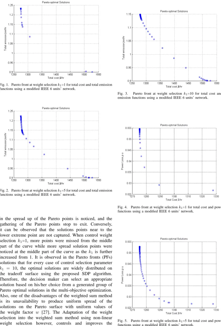
Fig. 3. Pareto front at weight selectionk1=10 for total cost and total emission functions using a modified IEEE 6 units’ network.
Fig. 4. Pareto front at weight selectionk1=1 for total cost and power loss functions using a modified IEEE 6 units’ network.
Fig. 5. Pareto front at weight selectionk1=5 for total cost and power loss functions using a modified IEEE 6 units’ network.
IAENG International Journal of Computer Science, 44:4, IJCS_44_4_10
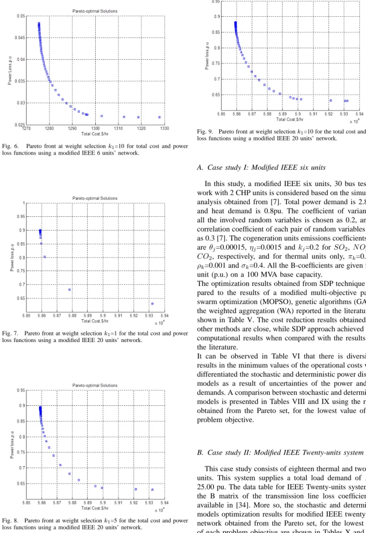
Fig. 6. Pareto front at weight selectionk1=10 for total cost and power loss functions using a modified IEEE 6 units’ network.
Fig. 7. Pareto front at weight selectionk1=1 for the total cost and power loss functions using a modified IEEE 20 units’ network.
Fig. 8. Pareto front at weight selectionk1=5 for the total cost and power loss functions using a modified IEEE 20 units’ network.
Fig. 9. Pareto front at weight selectionk1=10 for the total cost and power loss functions using a modified IEEE 20 units’ network.
A. Case study I: Modified IEEE six units
In this study, a modified IEEE six units, 30 bus test net-work with 2 CHP units is considered based on the simulation analysis obtained from [7]. Total power demand is 2.834pu and heat demand is 0.8pu. The coefficient of variance of all the involved random variables is chosen as 0.2, and the correlation coefficient of each pair of random variables is set as 0.3 [7]. The cogeneration units emissions coefficients used are θj=0.00015, ηj=0.0015 and kj=0.2 for SO2,N Ox and CO2, respectively, and for thermal units only, πk=0.0008, ρk=0.001 andσk=0.4. All the B-coefficients are given in per unit (p.u.) on a 100 MVA base capacity.
The optimization results obtained from SDP technique com-pared to the results of a modified multi-objective particle swarm optimization (MOPSO), genetic algorithms (GA) and the weighted aggregation (WA) reported in the literature are shown in Table V. The cost reduction results obtained from other methods are close, while SDP approach achieved better computational results when compared with the results from the literature.
It can be observed in Table VI that there is diversity of results in the minimum values of the operational costs which differentiated the stochastic and deterministic power dispatch models as a result of uncertainties of the power and heat demands. A comparison between stochastic and deterministic models is presented in Tables VIII and IX using the results obtained from the Pareto set, for the lowest value of each problem objective.
B. Case study II: Modified IEEE Twenty-units system
This case study consists of eighteen thermal and two CHP units. This system supplies a total load demand of PD = 25.00 pu. The data table for IEEE Twenty-units system and the B matrix of the transmission line loss coefficient are available in [34]. More so, the stochastic and deterministic models optimization results for modified IEEE twenty units network obtained from the Pareto set, for the lowest value of each problem objective are shown in Tables X and XI.
The Bij matrix of the transmission loss coefficient for
IAENG International Journal of Computer Science, 44:4, IJCS_44_4_10
TABLE V
COST REDUCTION ON A MODIFIEDIEEESIX UNITS’NETWORK INCORPORATING TWOCHPUNITS.
SDP MOPSO GA WA P1 0.0500 0.2980 0.4597 0.0500 P2 0.6000 0.4576 0.5290 0.6000 P3 0.5260 0.6519 0.4721 0.7737 P4 1.2000 0.7826 0.8623 0.7205 Θ1 0.4629 0.3468 0.4856 0.0600 Θ2 0.0500 0.1523 0.0699 0.0600 H1 0.0000 0.2422 0.3684 0.0000 H2 0.6000 0.2330 0.1507 0.2000 T1 0.2000 0.2972 0.2309 0.5000 Cost 1275.3 1305.0 1322.4 1303.6 CO2 1.0823 1.5960 1.7212 1.6001 N Ox,SO2 0.1519 0.1272 0.1285 0.1361 Power dev. 0.5265 0.4784 0.5447 0.4882 Heat dev. 0.0268 0.0309 0.0292 0.0206 TABLE VI
COST REDUCTION INCORPORATING TWOCHPUNITS CONSIDERING A MODIFIEDIEEESIX UNITS’NETWORK USINGSDPAPPROACH
Gen/Obj Sto. Model (SM) Det. Model (DM)
P1(P1) 0.0500 0.0828 P2(P2) 0.6000 0.6000 P3(P3) 0.5260 0.5086 P4(P4) 1.2000 1.2000 Θ1(Θ1) 0.4629 0.4493 Θ2(Θ2) 0.0500 0.0500 H1(H1) 0.0000 0.0000 H2(H2) 0.6000 0.6000 T1(T2) 0.2000 0.2000 Cost 1275.3 1274.3 CO2 1.0821 1.0836 N Ox,SO2 0.1519 0.1470 Total Emission 1.2340 1.2306 Power Loss 0.0531 0.0567 Power dev. 0.5265 0.5311 Heat dev. 0.0268 0.0268
Total Power Output 2.8871 2.8907
Total Heat Output 0.8000 0.8000
TABLE VII
COST REDUCTION ON A MODIFIEDIEEE TWENTY UNITS’NETWORK INCORPORATING TWOCHPUNITS USINGSDPAPPROACH
Gen/Obj Opt. val Gen/Obj Opt. val
P1 4.3094 P16 0.8000 P2 1.8332 P17 0.6618 P3 1.3017 P18 0.8610 P4 1.0920 Θ1 1.0000 P5 0.9691 Θ2 0.6000 P6 0.5924 H1 0.0000 P7 1.0950 H2 0.6000 P8 1.2927 T1 0.2000 P9 0.9415 Cost($/pu) 58593.0 P10 0.8183 Power Loss 0.9000 P11 1.4582 Power dev. 54.4161 P12 2.7944 Heat dev. 0.0268
P13 1.4293 Total Power Output 25.9000
P14 0.2000 Total Heat Output 0.8000
P15 1.8500
TABLE VIII
MULTI-OBJECTIVE MINIMIZATION RESULTS FOR STOCHASTIC MODEL CONSIDERING A MODIFIEDIEEESIX UNITS TEST SYSTEM USINGSDP
APPROACH
min{J1¯} min{J2¯} min{J3¯} min{J4¯} min{J5¯}
1275.3 1528.1 1422.1 1415.7 1327.9 1.2342 0.9013 1.2213 1.3585 1.3387 0.5265 0.5165 0.4567 0.5210 0.5482 0.0268 0.0416 0.0334 0.0256 0.0341 0.0546 0.1902 0.0873 0.0854 0.0267 TABLE IX
MULTI-OBJECTIVE MINIMIZATION RESULTS FOR DETERMINISTIC MODEL CONSIDERING A MODIFIEDIEEESIX UNITS TEST SYSTEM
USINGSDPAPPROACH
min{J1¯} min{J2¯} min{J3¯} min{J4¯} min{J5¯}
1274.3 1519.9 1420.4 1411.6 1345.9 1.2306 0.8881 1.2142 1.3516 1.3014 0.5311 0.5084 0.4551 0.5165 0.5287 0.0268 0.0416 0.0333 0.0256 0.0341 0.0567 0.1664 0.0907 0.0727 0.0259
IEEE six units is given by 0.1382 −0.0299 0.0044 −0.0022 −0.0010 −0.0008 −0.0299 0.0487 −0.0025 0.0004 0.0016 0.0041 0.0044 −0.0025 0.0182 −0.0070 −0.0066 −0.0041 −0.0022 0.0004 −0.0070 0.0137 0.0050 0.0033 −0.0010 0.0016 −0.0066 0.0050 0.0109 0.0005 −0.0008 0.0041 −0.0066 0.0033 0.0005 0.0244 (49)
Furthermore, Figs. 10 and 11 illustrate the performance of SDP technique on stochastic and deterministic models respectively by performing fifty-one (51) iterations which were investigated on standard modified IEEE six and twenty units’ networks with two CHP units to each of the networks. It is established that there is significant variation in the comparative convergence profiles for both stochastic and deterministic models presented in both Figs. 10 and 11 using a standard modified IEEE six units’ network with two CHP units and also, Fig. 12 shows a comparative convergence profiles for both stochastic and deterministic models considering a standard modified IEEE twenty units’ network with two CHP units. There is a deviation in the results of stochastic and deterministic models presented in Figs. 10, 11 and 12 as a result of random effect on the power generation systems. Therefore, in real life implementation,
TABLE X
MULTI-OBJECTIVE MINIMIZATION RESULTS FOR STOCHASTIC MODEL CONSIDERING A MODIFIEDIEEE TWENTY UNITS USINGSDPAPPROACH
Obj min{J1¯} min{J3¯} min{J4¯} min{J5¯} Cost 58593.0 59285.0 60129.0 59323.0 Power dev. 54.4161 52.9812 56.5431 53.5166 Heat dev. 0.0268 0.0332 0.0256 0.0332 Power Loss 0.9000 0.7419 1.0661 0.6298
TABLE XI
MULTI-OBJECTIVE MINIMIZATION RESULTS FOR DETERMINISTIC MODEL CONSIDERING A MODIFIEDIEEE TWENTY UNITS USINGSDPAPPROACH
Obj min{J1¯} min{J3¯} min{J4¯} min{J5¯}
Cost 29826 29834 29835 29834
Power dev. 8.5139 8.5139 8.5139 8.5139 Heat dev. 0.5937 0.5357 0.5297 0.5358 Power Loss 0.1436 0.1436 0.1436 0.1436
IAENG International Journal of Computer Science, 44:4, IJCS_44_4_10
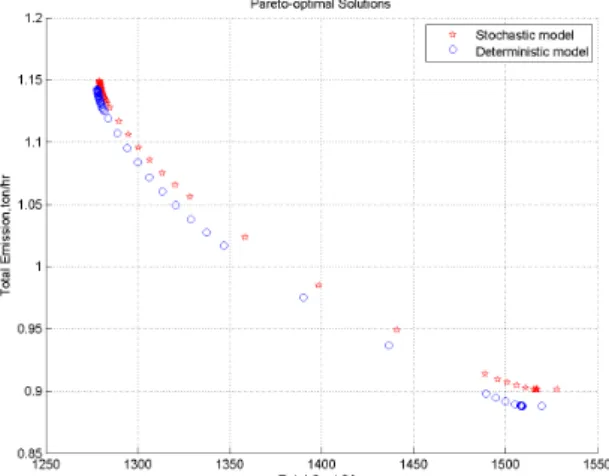
Fig. 10. Pareto fronts for the Stochastic and Deterministic models
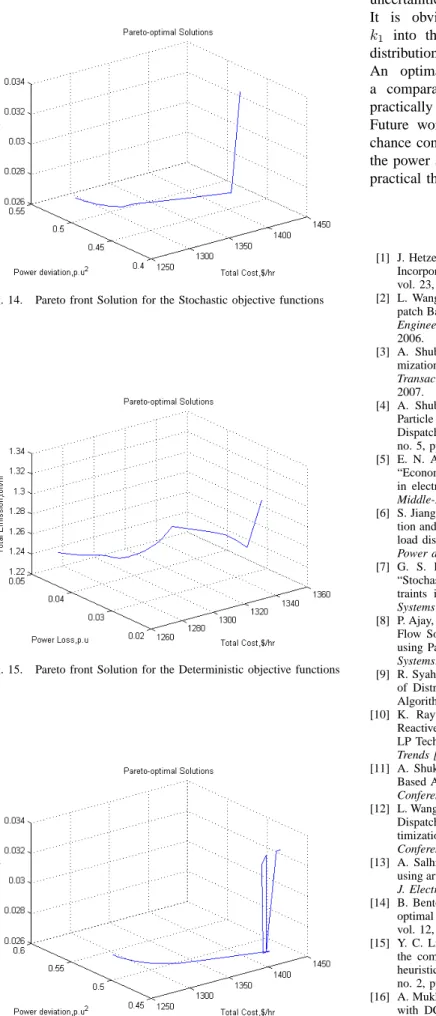
it is advisable to express problems in CHP as stochastic model so as to cover the effect of the uncertain factors [7]. Figs. 13 and 14 illustrate the Pareto fronts solutions for the simultaneous minimizations of stochastic multi-objective problems respectively. It is shown in Fig. 13 that the lower extreme solution produces the lowest total cost, at maximum power loss and minimum total emission, while at the upper extreme point generates maximum total cost at minimum power loss and maximum total emission among all the solutions in the Pareto front. Fig. 14 shows that the lower extreme solution generates lowest value of total cost, at maximum power deviation and minimum heat deviation whereas as the total cost increases, heat deviation increases and power deviation decreases among all the solutions in the Pareto front. If randomness is to be considered in the power systems, there will be increase in total cost, power and heat deviations [1].
Also, the Pareto solutions for the simultaneous minimization of deterministic multi-objectives functions are presented in Figs. 15 and 16. It can be deduced from the Fig. 15 that the lower extreme solution indicates that at minimum total cost, maximum power loss and minimum total emission are generated while at the upper extreme solution gives maximum total cost, at minimum power loss and maximum total emission among the solutions in Pareto front. On the other hand, Fig. 16 illustrates that at minimum total cost, maximum power deviation and minimum heat deviation are generated at the lower extreme solution.
VI. CONCLUSION
The proposed SDP method performed well in accuracy of results and provides lower operational cost in the Pareto set produced. The results for the multi-objectives formulation problems are presented using SDP approach, indicating that the decision maker can choose his/her preferred solution while satisfying multiple criteria. The SDP method solves a stochastic problem by minimizing the expectation of the multi-objective functions using the statistics of Gaussian distribution. Also, further investigations were performed on the comparison of the stochastic model for the multi-objective functions and the deterministic approach, resulting to diversity in total operational cost which covers the
Fig. 11. Pareto fronts for the Stochastic and Deterministic models
Fig. 12. Pareto fronts for the Stochastic and Deterministic models
Fig. 13. Pareto front Solution for the Stochastic objective functions
IAENG International Journal of Computer Science, 44:4, IJCS_44_4_10
Fig. 14. Pareto front Solution for the Stochastic objective functions
Fig. 15. Pareto front Solution for the Deterministic objective functions
Fig. 16. Pareto front Solution for the Deterministic objective functions
uncertainties of power and head demand.
It is obvious that the adaptation of weight selection
k1 into the weight sum method achieves more uniform
distribution of the solution points as thek1 value increases.
An optimal selection of k1 parameter that generates
a comparative uniform spread out of the algorithm is practically determined.
Future work can be conducted in the implementation of chance constraints to capture the stochastic characteristic of the power system generation and distribution which is more practical than the deterministic constraints.
REFERENCES
[1] J. Hetzer, D. C. Yu and K. Bhattarai, “An Economic Dispatch Model Incorporating Wind Power,” IEEE Transactions on Energy Conversion, vol. 23, no. 2, pp. 603-611, June 2008.
[2] L. Wang and C. Singh, “Stochastic Combined Heat and Power Dis-patch Based on Multi-Objective Particle Swarm Optimization,” Power
Engineering Society General Meeting, IEEE, vol. 8, no. 2, pp. 8-16,
2006.
[3] A. Shubham and B. K. Panigrahi, “A New Particle Swarm Opti-mization Solution to Nonconvex Economic Dispatch Problems,” IEEE
Transactions on Power Systems, vol. 22, no. 1, pp. 380-389, February
2007.
[4] A. Shubham, B. K. Panigrahi, and M. K. Tiwari, “Multiobjective Particle Swarm Algorithm With Fuzzy Clustering for Electrical Power Dispatch,” IEEE Transactions on Evolutionary Computation, vol. 12, no. 5, pp. 567-578, October 2008.
[5] E. N. Azadani, S. H. Hosseinian, B. Moradzadel and P. Hasanpor, “Economic dispatch in Multi-area using particle swarm optimization in electricity market,” Power System Conference, 12th International
Middle-East, pp. 559-564, 2008.
[6] S. Jiang, Z. Ji and Y. Shen, “A novel hybrid particle swarm optimiza-tion and gravitaoptimiza-tional search algorithm for solving economic emission load dispatch problems with various practical constraints,” Electrical
Power and Energy Systems, vol. 55, no. 2, pp. 628-644, 2014.
[7] G. S. Piperagkas, A. G. Anastasiadis and N. D. Hatziargyriou, “Stochastic PSO-based and power dispatch under environmental con-traints incorporating CHP and wind power units,” Electric Power
Systems Research, vol. 81, no. 1, 2010.
[8] P. Ajay, D. V. Raj, T. G. Palanivelu and R. Gnanadass, “Optimal Power Flow Solution for Combined Economic Emission Dispatch Problem using Particle Swarm Optimization Technique,” Journal of Electrical
Systems, vol. 3, no. 1, pp. 13-25, 2007.
[9] R. Syahputra, I. Soesanti and M. Ashari, “Performance Enhancement of Distribution Network with DG Integration Using Modified PSO Algorithm,” J. Electrical Systems, vol. 12, no. 1, pp. 1-19, 2016. [10] K. Rayudu, M. ali, G. Yesuratnam and A. Jayalaxmi, “Optimal
Reactive Power Dispatch Based on Particle Swarm Optimization and LP Technique,” International Conference on Emerging Technological
Trends [ICETT], 2016.
[11] A. Shukla, S. Kesherwani and S. N. Singh, “Efficient Holomorphic Based Approach for Unit Commitment Problem,” IEEE International
Conference, 2016.
[12] L. Wang, and C. Singh, “Tradeoff Between Risk and Cost in Economic Dispatch Including Wind Power Penetration Using Particle Swarm Op-timization,” Power System Technology, PowerCon 2006. International
Conference, pp. 1-6, 2006.
[13] A. Salhi, D. Naimi and T. Bouktir, “Optimal power flow resolution using artificial bee colony algorithm based grenade explosion method,”
J. Electrical Systems, vol. 12, no. 4, pp. 734-756, 2016.
[14] B. Bentouati, C. Chettih, P. Jangir and I. Trivedi, “A solution to the optimal power flow using multi-verse optimizer,” J. Electrical Systems, vol. 12, no. 4, pp. 30-36, 2016.
[15] Y. C. Liang and R. C. Juarez, “A normalization method for solving the combined economic and emission dispatch problem with meta-heuristic algorithms,” Electrical Power and Energy Systems, vol. 54, no. 2, pp. 163-186, 2014.
[16] A. Mukherjee and V. Mukherjee, “A Solution to Optimal Power Flow with DC Link Placement Problem using Chaotic Krill Herd Algo-rithm,” International Conference on Emerging Technological Trends
[ICETT], 2016.
[17] J. Wang and J. Song, “Chaotic Biogeography-based Optimization Algorithm,” IAENG International Journal of Computer Science, vol. 44, no: 2, pp. 25-32, 2017.
IAENG International Journal of Computer Science, 44:4, IJCS_44_4_10
[18] S. Li and J. Wang, “Improved Cuckoo Search Algorithm with Novel Searching Mechanism for Solving Unconstrained Function Optimiza-tion Problem,” IAENG InternaOptimiza-tional Journal of Computer Science, vol. 44, no: 1, pp. 301-314, 2017.
[19] K. R. Provas and B. Sudipta, “Multi-objective quasi-oppositional teaching learning based optimization for economic emission load dispatch problem,” Electrical Power and Energy Systems, vol. 53, no. 1, pp. 937-948, 2013.
[20] O. Herbadji, L. Slimani and T. Bouktir, “Solving Bi-Objective mal Power Flow using Hybrid method of Biogeography-Based Opti-mization and Differential Evolution Algorithm: A case study of the Algerian Electrical Network,” J. Electrical Systems, vol. 12, no. 1, pp. 197-215, 2016.
[21] J. Wang and J. Song, “A Hybrid Algorithm Based on Gravitational Search and Particle Swarm Optimization Algorithm to Solve Function Optimization Problems,” IEEE Engineering Letter, vol. 25, no: 1, pp. 20-25, February 2017.
[22] K. Jagatheesan, B. Anand, S. Samanta, N. Dey, A. S. Ashour, V. E. Balas,“Design of a proportional-integral-derivative controller for an automatic generation control of multi-area power thermal systems using firefly algorithm,” IEEE/CAA Journal of Automatica Sinica, pp. 1-14, 2017.
[23] N. Amjady, S. Dehghan, A. Attarha and A. J. Conejo, “Adaptive Ro-bust Network-Constrained AC Unit Commitment,” IEEE Transactions
on Power Systems, vol. 32, no. 1, pp. 672-683, January 2017.
[24] C. Shao, X. Wang, M. Shahidehpour and X. Wang, “An MILP-Based Optimal Power Flow in Multicarrier Energy Systems,” IEEE
Transactions on Sustainable Energy, vol. 8, no. 1, pp. 239-248, January
2017.
[25] C. Lin, W. Wu, B. Zhang, B. Wang, W. Zheng and Z. Li, “Decen-tralized Reactive Power Optimization Method for Transmission and Distribution Networks Accommodating Large-Scale DG Integration,”
IEEE Transactions on Sustainable Energy, vol. 8, no. 1, pp. 363-373,
January 2017.
[26] C. Yammani and V. K. Macha, “Fuel cost minimization with reserve capacity and inter-area flow limit for reliable and cost effective oper-ation of multi microgrids,” IEEE Region 10 Conference (TENCON) ˚U Proceedings of the International Conference, pp. 45-50, 2016.
[27] A. M. Jubril, “Economic-emission dispatch problem: A nonlinear weight selection in weighted sum for convex multiobjective optimiza-tion,” Facta Univ (NIS) Series Maths Inform, vol. 27, no. 3, pp. 357-372, 2013.
[28] J. Lavaei and S. H. Low, “Zero duality gap in optimal power flow problem,” IEEE Trans. Power Syst., vol. 27, no. 1, pp. 92-107, 2012. [29] R. A. Jabr, “Solution to economic dispatching with disjoint feasible regions via semidefinite programming,” IEEE Trans. Power Syst., vol. 27, no. 1, pp. 572-573, 2012.
[30] X. Bai, H. Wei, K. Fujisawa and Y. Wang, “Semidefinite programming for optimal power flowproblem,” Int. J. Electr. Power Energy Syst., vol. 30, no. 1, pp. 383-392, 2008.
[31] Z. Jin, F. Li, X. Ma and S. M. Djouadi, “Semi-Definite Programming for Power Output Control in a Wind Energy Conversion System,” IEEE
Transactions on Sustainable Energy, pp. 1949-1959, 2014.
[32] T. Ding, S. Liu, Z. Wu and Z. Bie, “Sensitivity-based relaxation and decomposition method to dynamic reactive power optimisation considering DGs in active distribution networks,” IET Generation,
Transmission and Distribution, vol. 11, no. 1, pp. 37 ˝U48, 2016. [33] S. Bahrami, F. Therrien, W. S. Wong and J. Jatskevich,
“Semidef-inite Relaxation of Optimal Power Flow for AC ˝UDC Grids,” IEEE
Transactions on Power Systems, vol. 32, no. 1, January 2017.
[34] L. S. Coelho and C. Lee, “Solving economic load dispatch problems in power systems using chaotic and Gaussian particle swarm optimization approaches,” Electric Power and Energy Systems, vol. 30, no. 2, pp. 297-307, 2008.
[35] S. Boyd and L. Vandenberghe, “Semidefinite Programming Relax-ations of Non-Convex Problems in Control and Combinatorial Op-timization,” Information Systems Laboratory, Stanford University, vol. 25, no. 1, pp. 29-37, 1997.
[36] S. Boyd and L. Vandenberghe, “Convex Optimization,” 1st ed., New
York: Cambridge University Press, 2004.
[37] S. Boyd and L. Vandenberghe, “Semidefinite Programming,” SIAM,
Rev., vol. 38, pp. 49-95, 2003.
[38] A. Aspremont and S. Boyd, “Relaxations and Randomized Methods for Nonconvex QCQPs,” Stanford University Autumn, 2003. [39] A. Rong and R. Lahdelma, “CO2 emissions trading planning in
combined heat and power production via multi-period stochastic optimization,” European Journal of Operational Research, vol. 176, pp. 1874-1895, 2007.
[40] A. Rong and R. Lahdelma, “Efficient algorithms for combined heat and power production planning under the deregulated electricity market,”
European Journal of Operational Research, vol. 176, pp. 1219-1245,
2007.
[41] F. Salgado and P. Pedrero, “Short-term operation planning on cogen-eration systems: A survey,” Electric Power Systems Research, vol. 78, no. 1, pp. 835-848, 2008.
[42] R. A. Abarghooee, T. Niknam, A. Roosta, A. R. Malekpour and M. Zare, “Probabilistic multiobjective wind-thermal economic emis-sion dispatch based on point estimated method,” Journal of Energy, vol. 37, no. 2, pp. 322-335, 2012.
[43] V. H. Quintana and M. Madriga, “Semi-Definite Programming Re-laxations for 0,1-Power Dispatch Problems,” University of Malaga,
Spain, vol. 21, no. 1, pp25-32, April 2000.