RESEARCH
Machine learning for high-throughput field
phenotyping and image processing provides
insight into the association of above and
below-ground traits in cassava (
Manihot
esculenta
Crantz)
Michael Gomez Selvaraj
1*, Manuel Valderrama
1, Diego Guzman
1, Milton Valencia
1, Henry Ruiz
2and Animesh Acharjee
3,4,5*Abstract
Background: Rapid non-destructive measurements to predict cassava root yield over the full growing season through large numbers of germplasm and multiple environments is a huge challenge in Cassava breeding programs. As opposed to waiting until the harvest season, multispectral imagery using unmanned aerial vehicles (UAV) are capable of measuring the canopy metrics and vegetation indices (VIs) traits at different time points of the growth cycle. This resourceful time series aerial image processing with appropriate analytical framework is very important for the automatic extraction of phenotypic features from the image data. Many studies have demonstrated the useful-ness of advanced remote sensing technologies coupled with machine learning (ML) approaches for accurate predic-tion of valuable crop traits. Until now, Cassava has received little to no attenpredic-tion in aerial image-based phenotyping and ML model testing.
Results: To accelerate image processing, an automated image-analysis framework called CIAT Pheno-i was devel-oped to extract plot level vegetation indices/canopy metrics. Multiple linear regression models were constructed at different key growth stages of cassava, using ground-truth data and vegetation indices obtained from a multispectral sensor. Henceforth, the spectral indices/features were combined to develop models and predict cassava root yield using different Machine learning techniques. Our results showed that (1) Developed CIAT pheno-i image analysis framework was found to be easier and more rapid than manual methods. (2) The correlation analysis of four pheno-logical stages of cassava revealed that elongation (EL) and late bulking (LBK) were the most useful stages to estimate above-ground biomass (AGB), below-ground biomass (BGB) and canopy height (CH). (3) The multi-temporal analysis revealed that cumulative image feature information of EL + early bulky (EBK) stages showed a higher significant cor-relation (r= 0.77) for Green Normalized Difference Vegetation indices (GNDVI) with BGB than individual time points.
© The Author(s) 2020. This article is licensed under a Creative Commons Attribution 4.0 International License, which permits use, sharing, adaptation, distribution and reproduction in any medium or format, as long as you give appropriate credit to the original author(s) and the source, provide a link to the Creative Commons licence, and indicate if changes were made. The images or other third party material in this article are included in the article’s Creative Commons licence, unless indicated otherwise in a credit line to the material. If material is not included in the article’s Creative Commons licence and your intended use is not permitted by statutory regulation or exceeds the permitted use, you will need to obtain permission directly from the copyright holder. To view a copy of this licence, visit http://creat iveco mmons .org/licen ses/by/4.0/. The Creative Commons Public Domain Dedication waiver (http://creat iveco mmons .org/publi cdoma in/ zero/1.0/) applies to the data made available in this article, unless otherwise stated in a credit line to the data.
Open Access
*Correspondence: [email protected]; [email protected] 1 International Center for Tropical Agriculture (CIAT), A.A. 6713 Cali, Colombia
3 College of Medical and Dental Sciences, Institute of Cancer and Genomic Sciences, Centre for Computational Biology, University of Birmingham, Birmingham B15 2TT, UK
Background
Cassava (Manihot esculenta Crantz), commonly referred
as manioc (French), yuca (Spanish), and different names in local regions, is a tropical root crop native to South
America [1], and relied by more than 800 million people
as a staple food source [2]. Its versatile nature, it is often referred to as the “drought, war and famine crop of the
developing world” [3], places it among the most
adap-tive crops during climate change. Early vigor, rapid root bulking, higher root yield, resistance to major pest and diseases, waxy cassava are the most important targeted
traits in cassava breeding programs around the world [4].
Conventional breeding continues to be the main method for cassava varietal development worldwide and had a strong impact on addressing the constraints of cassava
growers [5]. Traditional methods of selecting breeding/
germplasm lines are labor intensive and destructive to nature, limiting the quantitative and repeated
assess-ments in long-term research [6, 7]. Therefore,
estab-lishing a non-destructive and real time monitoring tool to measure above and below-ground cassava traits are
very necessary [8]. Exploring non–destructive selection
methods has always been a priority in cassava breeding programs. Therefore, efforts have been taken to reduce the cassava selection cycle and develop non-destructive, low-cost phenotyping methods that precisely
meas-ure the root characteristics in the field [8–12]. Though
good progress in digital phenotyping has been made, so far, no studies have been devoted to the development of non-invasive high-throughput field phenotyping (HTFP) tools and machine learning models that estimate cassava canopy traits and root yield prediction through aerial imaging. In cassava breeding programs, the establish-ment of non-destructive phenotyping tools, root yield prediction models can allow the early selection of elite genotypes, allowing the optimization of resources and
time [13]. Digital and rapid phenotyping approaches
are increasingly considered important tools for rapid
advancement of genetic gain in breeding programs [14].
UAV are being used to measure with high spatial and temporal resolution capable of generating useful
infor-mation for plant breeding tasks [15–17]. In the era of
digital revolution, aerial image phenotyping [18–20]
and ML models could predict crop yield performance
[21–27] in a non-invasive means with a greater
accu-racy [28–31]. Efficient selection of desired phenotypes
through HTP across large field populations could be achieved through incorporating ML methodologies such as, automated identification, classification,
quan-tification and prediction [20]. To be constructive to
breeding programs, phenotyping methods must be robust, automated, sensitive, and amenable to plot sizes. The ability to get more rapid growth responses of genetically different plants in the field and transmit these responses to individual genes, novel technologies such as proximal sensing, robotics, integrated compu-tational algorithms and robust automated aerial image
analytical frameworks are urgently needed [7].
Even though, UAV and sensor technologies (hard-ware) shows greater progress with more automation and integration, processing the massive amount of generated image data such as data management, image analysis, and result visualization of large-scale
pheno-typic data sets [32] from aerial phenotyping systems
requires robust analytical framework for data
interpre-tation [33]. Few commercial software are available that
systematize image calibration and correction, obtain-ing good field maps of the studied variable. But these platforms are often developed and delivered by specific enterprises where the original hardware and software are patent protected and henceforth cannot be adapted
or modified to meet particular research needs [34].
Moreover, new developments target real-time pro-cessing on-board in aerial imaging platforms, provid-ing direct vegetation indices (VIs) maps to make rapid
Canopy height measured on the ground correlated well with UAV (CHuav)-based measurements (r= 0.92) at late bulking (LBK) stage. Among different image features, normalized difference red edge index (NDRE) data were found to be consistently highly correlated (r= 0.65 to 0.84) with AGB at LBK stage. (4) Among the four ML algorithms used in this study, k-Nearest Neighbours (kNN), Random Forest (RF) and Support Vector Machine (SVM) showed the best performance for root yield prediction with the highest accuracy of R2= 0.67, 0.66 and 0.64, respectively.
Conclusion: UAV platforms, time series image acquisition, automated image analytical framework (CIAT Pheno-i), and key vegetation indices (VIs) to estimate phenotyping traits and root yield described in this work have great potential for use as a selection tool in the modern cassava breeding programs around the world to accelerate germplasm and varietal selection. The image analysis software (CIAT Pheno-i) developed from this study can be widely applicable to any other crop to extract phenotypic information rapidly.
Keywords: Automated aerial image processing, Above-ground biomass, Cassava, Machine learning, Multispectral UAV imagery, Root yield prediction
decisions [35]. Despite these improvements, there are middle steps that require some level of manual inter-face, which slow the progress, such as the recognition of coded GCP, calibration panel recognition and cor-rection, defining region of interest, extracting plot-level
data [32], batch and multi-threading processing.
In this paper, we are describing a robust feature extraction platform for aerial image processing called CIAT Pheno-i, with which we validated the developed framework using cassava time series aerial images col-lected from two consecutive field trials (2016–2018). Since no studies have been reported on UAV based cassava high-throughput phenotyping and root yield prediction, the specific objectives of this study is (1) to develop simple and rapid aerial image analysis frame-work (CIAT Pheno-i) for retrieving cassava canopy variables and VIs from multispectral (MS) time series images; 2) to find promising image based canopy
metrics and VIs to estimate above and below-ground biomass of cassava over different phenological stages; and (3) to develop robust ML models to predict cassava root yield using image features.
Materials and methods
Experimental site and trial conditions
To validate the performance of CIAT Pheno-i, two field trials, trial one was planted on December 2016 and harvested in November 2017; trial two was planted in December 2017 and harvested in December, 2018, these trials were conducted at the International Center for Tropical Agriculture (CIAT) headquarters Valle del
Cauca, Cali, Colombia at 970.67 m.a.s.l (3°30′29.21″N
− 76°20′53.98″W) (Fig. 1a). Climate and experimental
conditions were characterized for both trials (Table 1).
For both trials, we selected four contrasting geno-types GM3893-65, CM523-7, MPER-183, and HMC-1,
Fig. 1 Field trial site and remote sensing platform. a Trial one and two were conducted at the International Center for Tropical Agriculture (CIAT). b
Unmanned aerial vehicle (UAV), DJI S1000s. c Multispectral camera, Micasense RedEdge 3. d Arduino nano. e Ground Control Point (GCPs). f GCPs installed in trial one. g RTK-GPS
Table 1 Field experimental conditions and images acquisition
The following definitions are related to cassava storage root development phases: Elongation (EL) stage is the initial growth phase of active fibrous root development. Early bulking (EBK) is the root differentiation (from fibrous and storage roots) phase, the beginning of storage root bulking and accumulation of assimilated reserves in the storage roots. Late bulking (LBK) stage is the rapid expansion and bulking of storage roots. Dry matter accumulation (DMA) stage is the starch accumulation in the storage roots
Trial conditions and images acquisition Trial one (Dec. 2016–Nov. 2017) Trial two (Dec. 2017–Dec. 2018)
Irrigation Surface irrigation Drip irrigation
Soil type Clay loam Clay loam
Experimental design Split plot design Randomized complete block design
No. of replication 3 4
Average annual precipitation (mm) 1435.10 1026.50
Average annual temperature (°C) 24.00 23.33
Total solar radiation (W/m2) 207.8 222.39
Average annual relative humidity (%) 81.30 78.90
representing three types of canopy architecture;
cylin-drical, open and compact [36] and morphological and
agronomic growth descriptors are listed in Additional
file 1: Tables S1 and S2. The trial one was established in
0.8 hectares under a split-plot design with three
replica-tions and a total of 135 plots (3.0, long × 9.6 wide) with
staggered planting (Nine planting dates from December
2016 to August 2017) (Table 1). Cuttings were planted of
1.5 m between hills and 2.4 m between rows and water management was applied by the surface irrigation system
from planting to 7 months, using approximately 4000 m3
per hectare. The second trial was planted in 0.6 hectares with four replications per genotype and plot size of 9.6 m
long and 9.6 m wide (Table 1). Cuttings were planted of
1.2 m between hills and 2.4 m between rows and water management was applied with an efficient drip irrigation system from planting to 7 months, using approximately
900 m3 per hectare. In both trials, stem cuttings between
20 to 25 cm were planted vertically into the soil, leav-ing exposed three buds. Weeds were controlled by hand weeding, brush-cutter, and applying herbicides in late cassava stages. Standard agronomic, insects and diseases management practices were followed. A recommended dose of diammonium phosphate (DAP) and potassium chloride (KCL) were applied at the rate of 35.89 and 179 kg ha−1, respectively.
Ground‑truth measurements
Cassava agronomic traits such as leaf area index (LAI), canopy height (CH), above-ground biomass (AGB) and below-ground biomass (BGB) were acquired as ground-truth measurements. Five plants per plot were measured
using LICOR LAI-2200C Plant Canopy Analyzer [37]
during trial two. CH was sampled from soil level to the upper canopy at all four important phenological stages: elongation (EL), early bulking (EBK), late bulking (LBK) and dry matter accumulation (DMA) in both the trials.
Each phenological stage is defined in Table 1. CH of 21
and five plants per plot were measured in trial one and two, respectively. The AGB and BGB were measured at the harvest time in both the trials using a conventional scale with the accuracy of 1 g. For AGB, three and five plants per plot were sampled in trial one and two, respec-tively. For BGB, 15 and 45 plants per plot were sampled in trial one and two, respectively.
UAV platform and images acquisition
In this study, aerial multispectral (MS) time-series images were obtained using a MS camera (MicaSense RedEdge 3) mounted on a commercial UAV DJI S1000
octocop-ter (Fig. 1b). The MS camera has five spectral bands—
Blue, Green, Red, near-infrared (NIR), and Red Edge (RE) with the wavelengths of 455–495 nm, 540–580 nm,
658–678 nm, 800–880 nm and 707–727 nm, respectively
(Fig. 1c). The camera was attached to UAV by one plate
with a shock absorption rubber/spring damping suspen-sion system to protect against any vibration and to ensure better quality of the images. Six automated PhotoScan coded target detection (concentric rings) as ground
con-trol points (GCPs) were printed on a 50 × 50 cm plastic
sheet (Fig. 1e) and evenly distributed within the field
trial (Fig. 1f). These GCPs were georeferenced using
the highly accurate RTK-GPS (Real-Time Kinematic Global Positioning System, South, Galaxy G1, China) with a horizontal accuracy of 0.25 m and a vertical accu-racy of 0.5 m, which was used for geometric corrections
(Fig. 1g). These GCPs were maintained until all the UAV
images were acquired. The automatic fly mission was performed using DJI Ground Station Pro Application (DJI GS Pro, China). Before each image acquisition, one image was taken to the MicaSense reflectance panel for
radiometric calibration (Fig. 1h). Each image acquisition
was taken between 10:00 to 14:00 UTC-05:00. In order to achieve overlapping of 75% vertically and horizontally, we triggered the camera using the UAV DJI A3 flight controller and Arduino Nano as an interface configured
by DJI GS app (Fig. 1d). The altitude for image
acquisi-tion was between 30 and 40 m above ground level (from 2.7 to 5.4 cm per pixel). DJI S1000, batteries, and multi-sensors weights 3 kg. DJI S1000 UAV includes a Global Navigation Satellite System (GNSS), an inertial measure-ment unit (IMU), barometer and compass; all these com-ponents aid in position accuracy and vertical stability of the UAV during image acquisitions. The time series UAV images captured at different phenological stages at trial
one and two are listed in Table 1 and these acquired time
series images used to create the orthomosaic employed structure from motion (SfM) were listed in Additional file 1: Tables S1 and S2.
Image data processing
Generation of orthomosaic and digital elevation models
To ensure the reflectance quality of the orthomosaic, we followed the steps suggested by Agisoft and MicaSense
RedEdge cameras (Agisoft, https ://bit.ly/32swt n2). These
steps include the usage of the MicaSense downwelling light sensor to fix any illumination issues caused by the weather conditions and MicaSense reflectance calibra-tion panel. The acquired images were processed through Agisoft MetaShape Pro software (Version 1.2.2, Agisoft
LLC, http://www.agiso ft.com) and its Python API
(Appli-cation Program Interface) generates and exports a five-band orthomosaic and digital elevation models (DEM) automatically as GeoTIFF format. Our processing work-flow includes following nine main steps (1) Uploading UAV images, (2) calibration, (3) GCPs detection and
geo-tagging, (4) photo alignment, (5) camera optimiza-tion (6) build dense point cloud, (7) build DEM, (8) build orthomosaic (9) export DEM and orthomosaic
(Addi-tional file 2: Figure S1). In step three, coded GCPs are
automatically detected through Agisoft Metashape API (Fig. 1e).
Comparison of manual and automatic orthomosaic and DEM generation
In order to evaluate the efficiency of the Agisoft Metashape Python API, we generated orthomosaic and DEM using manual (M1–M8) and auto mode (A1–A8) from MS and RGB datasets. All data sets (MS and RGB) were processed using the image processing workflow listed in Additional file 2: Figure S1.
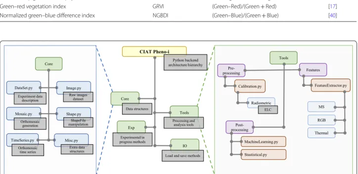
CIAT Pheno‑i image analysis framework
The CIAT Pheno-i is a web-based application (http://
pheno -i.ciat.cgiar .org/), designed to extract UAV derived vegetation indices (VIs) and canopy metrics
such as canopy height (CHuav), canopy cover (CCuav) and canopy volume (CVuav) rapidly. Canopy height defines the 95th percentile pixel height of the canopy point cloud. Canopy cover is the pixel surface area cov-ered by the canopy. Canopy volume, is the total volume under observed canopy values, which is derived as
fol-lows n
i CCuavi∗CHuavi where i is the pixel
associ-ated to the plot. CIAT Pheno-i admits MS orthomosaics and DEM as an input and visualizes them as VIs maps
(Additional file 2: Figure S2). Users have the privilege to
select their Region of Interest (ROI) using shapefiles and perform radiometric calibration, if necessary. Currently, eight VIs (Table 2) [17, 38–43] and three canopy metrics could be rapidly generated through Pheno-i and users can visualize real-time data captured over multiple tim-ing points durtim-ing the crop development.
CIAT Pheno‑i software architecture
CIAT Pheno‑i back‑end On the top of a PostgreSQL
data-base model, two main components constitute the Pheno-i
Table 2 Summary of vegetation indices used in this study. Camera channels B: blue, G: green, R: red, RE: red-edge, and NIR: near-infrared
Vegetation index Acronym Formula References
Normalized difference red-edge NDRE (NIR-Rededge)/(NIR + Rededge) [38] Normalized difference vegetation index NDVI (NIR-Red)(NIR + Red) [39] Green normalized difference vegetation index GNDVI (NIR-Green)/(NIR + Green) [40] Blue normalized difference vegetation index BNDVI (NIR-Blue)/(NIR + Blue) [41] Normalized difference vegetation index red-edge NDREI (Rededge-Red)/(Rededge + Red) [42] Normalized pigment chlorophyll index NPCI (Rededge-Blue)/(Rededge + Blue) [43] Green–red vegetation index GRVI (Green–Red)/(Green + Red) [17] Normalized green–blue difference index NGBDI (Green–Blue)/(Green + Blue) [40]
CIAT Pheno-i Python backend architecture hierarchy Exp Core Data structures Experimental/in progress methods IO Load and save methods
Tools DataSet.py Mosaic.py Core Experiment data description Image.py Raw images dataset Orthomosaic generation Shape.py ShapeFile manipulation TimeSeries.py Orthomosaic time series Misc.py Extra data structures Tools Features Pre-processing FeatureExtractor.py MS RGB Thermal Calibration.py Radiometric ELC Post-processing MachineLearning.py Stastistical.py Processing and analysis tools
back-end: A Python library, where the core algorithms in
the pipeline were implemented (Figs. 2 and 3), and a REST
(REpresentational State Transfer) API that allows the data processing through HTTP protocol. Most of the functions in the library were optimized using Numba, a python package that translates Python functions to optimized machine code, which could be executed in a parallel way on the CPU or the GPU. In addition to this, geo-spatial data manipulation, machine learning algorithms, GDAL, and Scikit-Learn were also employed. The following steps described below were coded in the CIAT Pheno-i python library:
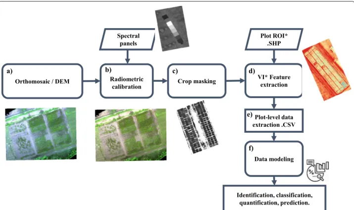
Step 1. Radiometric calibration: Using
orthomosa-ics (Fig. 3a), Pheno-i back-end implements
Empiri-cal Line Calibration (ELC) process (Fig. 3b) using
ground targets, allowing the user to calibrate ortho-mosaics after the flight. Before implanting the ELC process, the pixel digital numbers should range from 0 to 65,535 corresponding to a 16-bit standard Geo-TIFF format, after applying ELC the pixel values were converted to reflectance values between 0 and 1. Step 2. Crop masking and Vegetation indices cal-culation: To segment cassava canopy, the green
minus red (GMR) processing was used [44]. The
binarization of GMR was determined by the Otsu method to perform clustering-based image
thresh-olding [45], which implies the reduction of a gray
level image to two-pixel values (0 and 1) and this binary image was used to select and discard the
pixels associated with the soil (Fig. 3c). Using five
camera channels (B: blue, G: green, R: red, RE: red-edge, and NIR: near-infrared), eight normalized
vegetation indices (VIs) were intended (Table 2.)
Step 3. Plot-level data extraction: Using the cali-brated version of the orthomosaic, the boundaries of each plot ids are defined using an ESRI Shapefile format polygon. Then, shapefile was further used to select and extract the pixel values to compute sta-tistics such as mean, variance, median, standard
deviation, sum, minimum and maximum (Fig. 3e).
CIAT Pheno‑i web A single page app (SPA) was
devel-oped using React.js and Redux. This web application can be executed using any modern web browser (IE 11, Edge ≥ 14, Firefox ≥ 52, Chrome ≥ 49, Safari ≥ 10). The
user interface follows the Material-UI v4.7.0 (https ://
mater ial-ui.com/) guide design, LeafletJS v1.6.0 API (https ://leafl etjs.com/) was used to draw the
geo-refer-Orthomosaic / DEM Plot-level data extraction .CSV Data modeling Identification, classification, quantification, prediction. Plot ROI* .SHP Radiometric
calibration Crop masking
VI* Feature extraction Spectral panels a) b) c) d) e) f)
Fig. 3 CIAT Pheno-i workflow: Applying image processing for plot level data generation and use it on identification, classification, quantification and prediction
enced orthomosaics and polygons in an OpenStreetMap (https ://www.opens treet map.org/). Additional file 2: Figures S3 and S4 shows the overall architecture and database schema implemented.
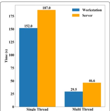
CIAT Pheno‑i back‑end performance To evaluate the
CIAT Pheno-i back-end performance, a single and multi-thread analysis were performed under server and work-station platforms over 50 different datasets. Hardware
and software specifications are listed in Additional file 1:
Table S3.
Statistical analysis
To investigate the relationship between agronomic traits, VIs and canopy metrics, we conducted Pearson correla-tions, where the traits were calculated using a pearsonr
function from Python SciPy (https ://www.scipy .org/)
package. Pearson’s correlation coefficients and a P value
less than 0.05 was considered significant.
Dataset preparation
In order to validate Pheno-i analysis, a Comma Separated Values (CSV) file with 693 characteristics was generated. Four machine-learning algorithms such as Support Vec-tor Machine (SVM), k-Nearest Neighbours (kNN), Ran-dom Forest (RF) and Artificial Neural Networks (ANN) were evaluated to predict cassava root yield. For the pre-processing, data scaling between -1 and 1 and a Box Cox transformation were performed to achieve a normal
dis-tribution [46]. Principal component analysis (PCA) and
principal component regression (PCR) [47] was applied
to compare performance and reduce the model com-plexity providing a lower-dimensional representation of predictor variables and to avoid multi-collinearity
between predictors [48–50]. To analyze the data at
dif-ferent growth stages, a multi-temporal VIs technique was
applied [27]; this procedure increases the predictor
vari-ables from 77 to 693 per timing point accumulating the VIs value per phenological stage.
Machine learning (ML) model development
ML model used
We included four ML methods in our study and are briefly described below. These ML methods were used in the regression mode.
Random forest Random forest method is a
non-para-metric, supervised method, that can be used as both clas-sification and regression. The heart of tree-based learners is the decision tree, wherein a series of decision rules are chained and learned. In a decision tree, every decision
rule occurs at a decision node [51]. This model was
pro-posed by Tin Kam Ho and further adapted by Leo
Brei-man and Adele Cutler [52].
Support Vector Machine Support Vector machines
[53] classify data by finding the hyperplane that
maxi-mizes the margin between the classes in the train-ing data. A support vector machine can be represented like:f(x)=β0+i∈SαiK(xi,xî) , where β0 is the bias,
S is the set of all support vector observations, α is the
parameters in the model to be learned, (xi,xî) are pairs of
two support vector operations and K is the kernel func-tion which compares the similarity between xi,xî.
k Nearest Neighbors The k-nearest Neighbors algorithm
[54] is a supervised machine learning algorithm that can
be used as both classification and regression problems, especially when there is little or no prior knowledge about
the distribution of the data. Let Xi be an input sample
with p features
xi1,xi2,. . .xip
, The Euclidean distance between the sample xi and xl(l=1, 2,. . .,n) is defined
as d(X1,Xl)= (xi1−xl1)2+ · · · + xip−xlp 2 ,
and its neighborhood as:
Ri=
X∈Rp:d(X,Xi)≤:d(X,Xm),∀i�=m
, where
Ri represents the clusters of elements with class m , and
X the set of points belong to it. The predicted class of
the new sample x is set equal to the most frequent class
among the k nearest training samples, which follow the rule:d(mi,X)=
d(mi,X)
, where d is the distance func-tion.
Multi‑Layer perceptron (MLP) A MLP is composed of
multiple perceptrons or neurons, developed originally by
Frank Rosenblatt [51], commonly arranged in three
lay-ers known as input layer, hidden layer (can have more than one stack of neurons) and output layer, and this kind of configuration is called Artificial Neural
Net-work (ANN). Each input of the neurons xi are
associ-ated with a weight wi and computed as a sum as follows
z=x1w1+ · · · +xnwn=XTW , then an activation
func-tion is calculated as f(z) , where f(z) can be any
continu-ously differentiable function like a linear function, sig-moid or even the modern ReLU commonly used in deep learning [55].
Assessing the quality of the model
Based on the experimental field design, a total of 609 samples were used to develop the models, three data repetitions (454 samples) were used to train and, one last repetition to test (155 samples). Regression model hyper-parameters were tuned using grid-search with ten-fold cross-validation to reduce variability and over-fitting
while modeling; methods provided with scikit-learn Python package. To assess the accuracy and performance between models root median square error (RMSE), relative root mean square error (RRMSE) and the
coef-ficient of determination (R2) were used. Ten-fold
cross-validation was performed over SVM, RF and kNN to get optimal hyper-parameters that minimize the error and stochastic gradient descendant over ANN model to reduce the training error.
Results and discussion
CIAT Pheno–i: an automated image analysis framework for HTFP
The increased use of UAVs in field phenotyping consid-erably decreased the hardware costs, however, image processing is the major challenge to the crop
phenotyp-ing scientists around the world [56]. As mentioned in the
introduction, midway steps to extract information from the plot level field experiments need full automation and integration. Therefore, a need for accurate, robust, and automated analysis framework building orthomosaics and extract phenotyping information corresponding to each image of micro-plots (breeding) or large scale (pre-cision agriculture) field experiments is necessary. Here, we are describing the Pheno-i image analysis software
(Additional file 3) developed by CIAT phenomics
plat-form (https ://pheno mics.ciat.cgiar .org/) and the
auto-mated orthomosaic generation pipeline. The primary criterion for any image analysis software should be cost effective, easy-to-use and rapid generation of actionable data from time-series images irrespective of experimen-tal plot sizes. Making use of Agisoft Metashape Python API, the orthomosaic and DEM generation process
was automated (Additional file 2: Figure S1),
achiev-ing a reduction in time of ~ 30%, savachiev-ing ~ 1.1 h for RGB
imagery and ~ 0.33 h for MS imagery (Additional file 2:
Figure S5), compared to our manual processing method. CIAT Pheno-i back-end image analysis software design brings a significant improvement over any regular single thread Python implementation reducing the processing
time of MS imagery processing up to 5× (Fig. 4).
Afore-said processing time was calculated using two different
CPU architectures as seen in Additional file 1: Table S3.
Our CIAT Pheno-i front-end software design comes with the advantage for the user to create, upload, calibrate, vis-ualize, and analyze orthomosaics in a map-based canvas, giving a privilege to a non-programmer to analyze his own data through the internet. The image analysis report comes in CSV format with a timestamp and a reference to a quantified plot level data, in which the data can be used either to develop plant models or just to monitor the crop health status. We offered CIAT Pheno-i as a
simple and easy to use solution to extract plot/plant-level information.
We validated the developed platform using proof-of-concept experiments with cassava genotypes over the two seasonal field trials to demonstrate the end-to-end application. The results obtained from the platform are described below.
High‑throughput field phenomics for aerial imaging of cassava
UAV offers very attractive alternatives such as, con-venient operation, high spatial and temporal
resolu-tions with reasonable spatial coverage [57–59], makes
it possible to document the within-microplot
variabil-ity in phenotyping field experiments [60, 61]. UAV, a
current and an invaluable tool for crop monitoring at
large scale (e.g., [27, 59, 62–65], has been proved to
be useful for estimating canopy height and biomass in
crops including rice [65], wheat [66] maize [30],
sor-ghum [67] and peas [17]. However, in cassava, the UAV
based high-throughput phenotyping methods need to be standardized for feasibility and accuracy in estimat-ing various phenotypestimat-ing parameters such as, biotic and abiotic stresses. So far, most studies have attempted to
Fig. 4 CIAT Pheno-i back-end performance. Multispectral 5 band image analysis average time of 50 runs with 3870 × 3739 pixels. Workstation processing time compared against server processing time
correlate morpho-physiological data with the produc-tive potential (root yield) of the genotypes at the end
of the crop cycle [68]. Subsequently, these
pre-breed-ing field experiments go through long selection cycles, leading to high maintenance costs. The correlation analysis between important breeding traits at differ-ent phenological stages and UAV image derived VIs are discussed below.
Relationship between UAV images derived features and canopy height
Canopy height (CH) is a key factor in cassava root
yield, dry matter, leaf area, and plant architecture [69].
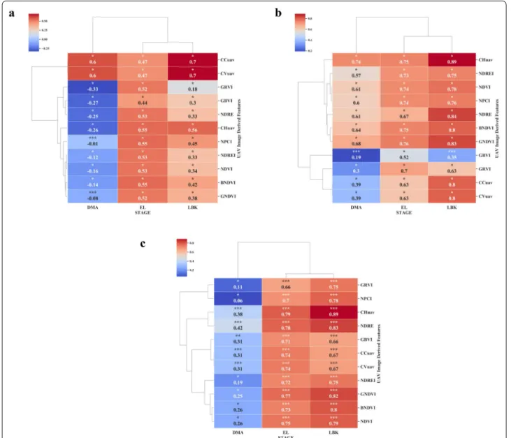
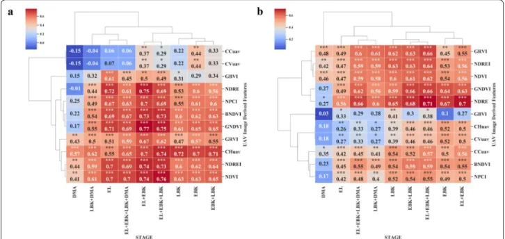
Collecting CH within cassava field breeding programs are labor intensive and prone to assessment error. In this study, orthomosaics and DEMs were generated using Methashape Agisoft API. Canopy metrics (CHuav, CCuav and CVuav) and VIs derived from high-resolu-tion MS images (2.7 cm x pixel) were extracted through our CIAT Pheno-i web-based application. The pearson’s correlation analysis between UAV features (VIs, CHuav, CCuav and CVuav) and canopy height (CH) at EL and LBK stage showed that the UAV feature are positively
correlated (Figs. 5c and 6a), except during the trial two,
where most of the VIs showed low and negative
correla-tions at DMA stage (Fig. 6a). This low or poor correlation
Fig. 5 Pearson correlation analysis between remote sensing features versus shoot and root biomass at different cassava phenological stages under surface irrigation management during the trial one. a BGB. b AGB. c CH. P < 0.05: *, P < 0.01: **, P < 0.005: ***
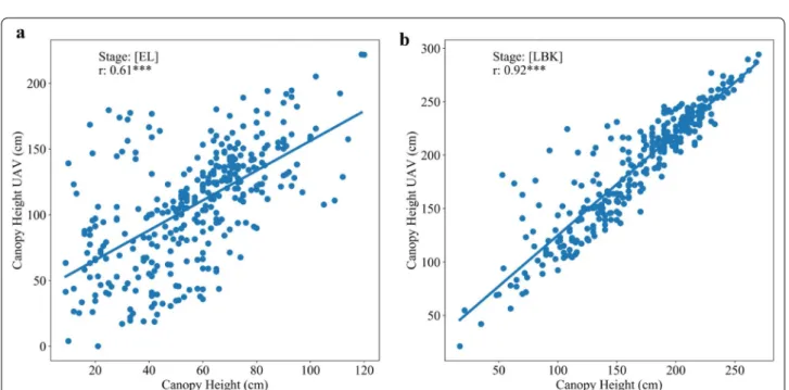
is mainly due to the saturation of VIs at later stages of growth and crop lodging. Significant correlation was found at EL stage between manually estimated CH and
CHuav (Fig. 7a). However, the best relationship was
reached at the late bulking stage for both the trials with r values 0.89 and 0.92, respectively (Figs. 5c, 6a, and 7b).
Similar results were found in cotton using DEMs from
MS cameras [70]. In trial one, among the VIs, NDRE
index showed significant relationship with CH manu-ally with an r value of 0.83 at LBK stage (Fig. 5c). The CH data collected by the UAV were credible and the corre-lation with ground-truth measurement was very high.
Fig. 6 Pearson correlation analysis between remote sensing features versus canopy metric traits at different cassava phenological stages under drip irrigation management during the trial two. a CH. b LAI. P < 0.05: *, P < 0.01: **, P < 0.005: ***
Therefore, UAV based CH measurements in cassava has great potential for use in studies of physiological and genetic mapping experiments.
Relationship between UAV metrics and canopy structure related traits
Time series measurements of canopy related traits are very useful to develop crop growth curves. Estimating AGB traits such as canopy volume is laborious, destruc-tive and time-consuming and therefore needs an easier
and convenient method [71]. In cassava, AGB can
pro-vide valuable insights into understanding the carbon assimilation mechanism and storage root development. In this paper, canopy metrics such as CCuav and CVuav across the phenological stages showed positive signifi-cant relationship with AGB. During the trial one and two, significant correlation (r = 0.80 and r = 0.54, respec-tively) was found between CCuav and AGB at LBK stage
(Figs. 5b and 8b). A similar relationship was previously
reported between dry leaf biomass and UAV derived
green CC [72]. Also, at LBK stage a similar relationship
(r = 0.70) was found between CVuav and BGB during the
trial one (Fig. 5a). High-throughput canopy metrics tools
developed from this study could provide quantitative data for novel traits that define canopy structure. Recur-rent measurement offers time-series data from which we can estimate growth rates and dynamics. Such non-inva-sive measurements are very useful to understand geno-type specific responses to environmental stresses during the growth period. Cassava canopy structure parameter
data can also contribute to the development of root yield prediction models and could help cassava breeders in the selection procedure by providing early hints on the per-formance of novel lines.
Correlation between LAI and UAV derived features
The leaf area index (LAI) refers to the per unit area of the one-sided leaf per unit area of ground surface. The maximum LAI in cassava ranges from 4 to 8, depending on the cultivar, the atmospheric and edaphic conditions
that prevails during crop growth stages [73]. Selection
for higher LAI should favor high root yield, since there is an optimum relationship between root yield and LAI
[68]. Positive contribution of LAI with cassava yield
has also been reported by [74], and [75] also reported
significant high correlation between ground cover and LAI in grass, legume and crucifer crop. Measuring LAI
is a tedious [76] and time-consuming process, and an
image trait complimenting LAI can be very useful. In order to establish this relationship, in trial two, LAI was measured and the correlation analysis was performed with UAV derived canopy metrics and VIs. The results of canopy metrics (CCuav and CVuav) and VIs showed highly significant and positive correlation with LAI in all the tested phenological stages, whereas, CCuav
and CVuav correlated with DMA with r value of 0.56
(Fig. 6b). Among the tested VIs, NDREI showed highly
significant correlation with LAI at EL and DMA stage
with r values of 0.53 and 0.63, respectively (Fig. 9a, d);
whereas, the correlation decreased slightly with the
Fig. 8 Pearson correlation analysis between remote sensing features versus shoot and root traits at different cassava phenological stages under drip irrigation management during the trial two. a BGB. b AGB. P < 0.05: *, P < 0.01: **, P < 0.005: ***
bulking stages (EBK and LBK) (Fig. 9b, c). Additionally, highly significant correlations were found with LAI and
NDVI at EL and DMA stages with r values of 0.55 and
0.59, respectively (Fig. 6b). Strong correlation between
NDVI and LAI using UAV images has also been
reported in different crops such as rice [65], sorghum
[67]; for NDREI in bread wheat [77]. These results
indi-cate that NDREI could explain the green leaf area dur-ing senescence.
Relationship between UAV features and above‑ground biomass
Breeding for early vigor, fast growing cassava genotypes is ideal to tackle several issues especially in early stages of crop management. Vigorous and early growth cul-tivars were less sensitive to lack of weed control than non-vigorous slow growth types. Above-ground biomass (AGB) estimation in cassava, is a most laborious and time-consuming method, requires a multi-step process: crop sacrifice from the field plot, oven dried before being
Fig. 9 Comparison of Normalized Difference Vegetation Index Red-Edge NDREI versus Leaf Area Index (LAI) at EL (Elongation), EBK (Early Bulking), LBK (Late Bulking), and DMA (Dry Matter Accumulation) of cassava during the trial two
weighed to assess the fresh and dry biomass of each sam-ple. This multi-step destructive process is prone to error, from variability in the area within the plot sampled, to the potential loss of material while collecting and
trans-porting [6]. In this present study, we estimated fresh
canopy biomass in cassava using remote aerial imaging methods. Our results from both the trials revealed sig-nificant positive correlations between VIs (NDRE, NDVI, GNDVI, BNDVI, NDREI, NPCI and GRVI) and AGB, at three different phenological stages (EL, EBK and LBK). A further comparison between VIs and AGB at LBK stage, using NDRE values alone, also showed positive
significant correlation in both the trials with r values of
0.84 and 0.65, respectively (Figs. 5b, 8b continuously dif-ferentiable function like a linear function). Across UAV derived canopy metrics at LBK stage, we found
signifi-cant correlation between CCuav and AGB above r = 0.54
(Figs. 5b, 8b). Our results clearly indicate that EBK is one of the key phenological stages to predict AGB through remote sensing in cassava. Combining VIs at three phe-nological stages (EL, EBK and LBK), the trial two showed good AGB relationship with NDRE, NDVI, GNDVI,
BNDVI, NDREI, NPCI and GRVI with r values of 0.71,
0.62, 0.66, 0.59, 0.64, 0.55, and 0.66, respectively (Figs. 8b and 10a).
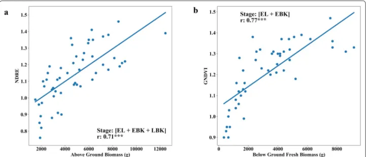
Relationship between UAV derived VIs and below‑ground biomass
Measuring root biomass through non-destructive meth-ods over different cassava varieties will help cassava
breeders in the efficient selection of cultivars with favora-ble rooting architectures e.g. root area and harvesting
[78]. Thereby, the impact of agronomic research through
unique agricultural practices on root bulking can be assessed. Destructive root sampling in cassava requires sampling large populations and trials that are laborious
and expensive [8]. Rapid and non-destructive process of
estimating below-ground biomass (BGB) across differ-ent environmdiffer-ents would reduce time, cost and sample size requirements in phenotypic data collection. In this study, we determine the capability of MS aerial imaging to estimate BGB. In both trials, except at DMA stage, all the tested VIs showed positive and significant
cor-relation with fresh BGB at EL and LBK stages (Figs. 5a,
8a). Our results revealed that the later stage (DMA) of
cassava crop life was least correlated, attributing the fact that at the later crop stages (i.e. when the roots are actively accumulating dry matter), cassava canopy tends to senescence.
In both the trials, NDRE, NDVI, GNDVI, BNDVI, NDREI, NPCI, GRVI indices showed significant positive
correlations with fresh root biomass with r values
rang-ing from 0.18 to 0.72 durrang-ing the EL to LBK stage, where
the highest correlation coefficient (r = 0.72) correspond
to NDRE at the EL stage at trial two (Figs. 5a and 8a).
On the other hand, canopy metrics (CCuav and CVuav) exhibited highest and stronger correlations with BGB at LBK in trial one with r = 0.70 and r = 0.70, respectively
(Fig. 5a). Also, we found that the DMA stage showed
poor and no significant correlation for some VIs, CHuav
Fig. 10 Relationship between fresh above-ground biomass (AGB) and fresh below ground biomass (BGB) of cassava with multi-temporal VIs (Normalized Difference Red-Edge, NDRE and Green Normalized Difference Vegetation Index GNDVI) during trial two. a Ground truth AGB versus multi-temporal NDRE index at EL (Elongation), EBK (Early Bulking), and LBK (Late Bulking stage). b Ground truth BGB and multi-temporal GNDVI index at EL (Elongation) and LBK (Late Bulking) stage
and CVuav metrics (Fig. 8a). In addition, the multi-temporal analysis showed improved correlations with BGB, where we observed that the combination of VIs at
[EL + EBK] stages showed highly significant correlation
(r= 0.77) for GNDVI (Figs. 8a and 10b). Generally, from
3 to 5 months after planting (MAP), intense development of the photosynthetic apparatus and aerial part of the cassava plants is observed. Consequently, a vigor in this phase causes the greatest enhancement of AGB with
con-sequent reflection in fresh root yield [13]. The
relation-ship between aerial imaging features and BGB obtained from this study are encouraging and it can be an add-on feature for our add-ongoing Ground penetrating Radar (GPR) research predicting BGB in cassava. Furthermore, all the data produced from above (UAV multispectral) and below ground sensors (GPR) could be merged using high precision Geographic Information System (GIS) to achieve more comprehensive estimation of BGB.
Cassava root yield predictions using ML models
Accurate estimation of crop yield is essential for plant breeders. Yield is a very important harvest trait observa-tion that involves the cumulative effect of weather and management practices throughout the entire growing
cycle. [79]. Early detection and crop management
asso-ciated with yield limitations can help increase produc-tivity [4, 23, 80]. Crop yield prediction models could aid in early decision-making, optimizing the time required for field evaluation, thus reducing the resources
allo-cated to the research programs [81]. Furthermore, the
predicted yield maps could also be used to implement variable rate technology (VRT) systems in spatial data-bases, thereby accomplishing precise field-level inputs
through the entire field [82]. Traditional cassava growth
models have certain limitations, such as high input cost required to run the models, the lack of spatial
informa-tion, or the actual quality of input data [13]. Remote
sensing approaches can provide growers with final yield
assessments and show variations across the field [79]. In
remote sensing, MS imagery can describe crop develop-ment for potato tuber yield forecasting, across time and space, in a cost-effective manner [81, 82].
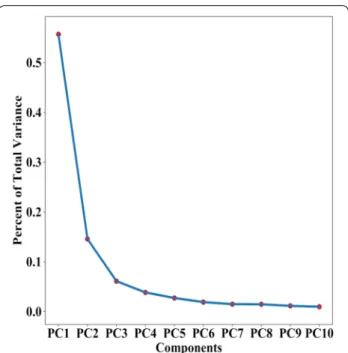
To our knowledge, there are no predictive models for cassava root yield using aerial imaging and ML tech-niques. Therefore, ML technique was explored to pro-vide a means of early prediction of cassava root yield using MS UAV remote sensing on a field scale. A PCA and PCR analysis was used to establish, with which more than 600 predictor variables were retained to train the models. The PCA results showed that the contribu-tion of the first 10 components explains 90% of variance
(Fig. 11) and PCR after a 10 fold cross validations can
achieve a R2 of 0.89. With PCA, the most important
component was PC1, explained 55.6% of total variance
(Table 3). Using the first four components provided by
PCA (80% of the total variance) and PCR, SVM, RF, kNN, and ANN models were built to predict BGB using multi-temporal VIs combinations and canopy
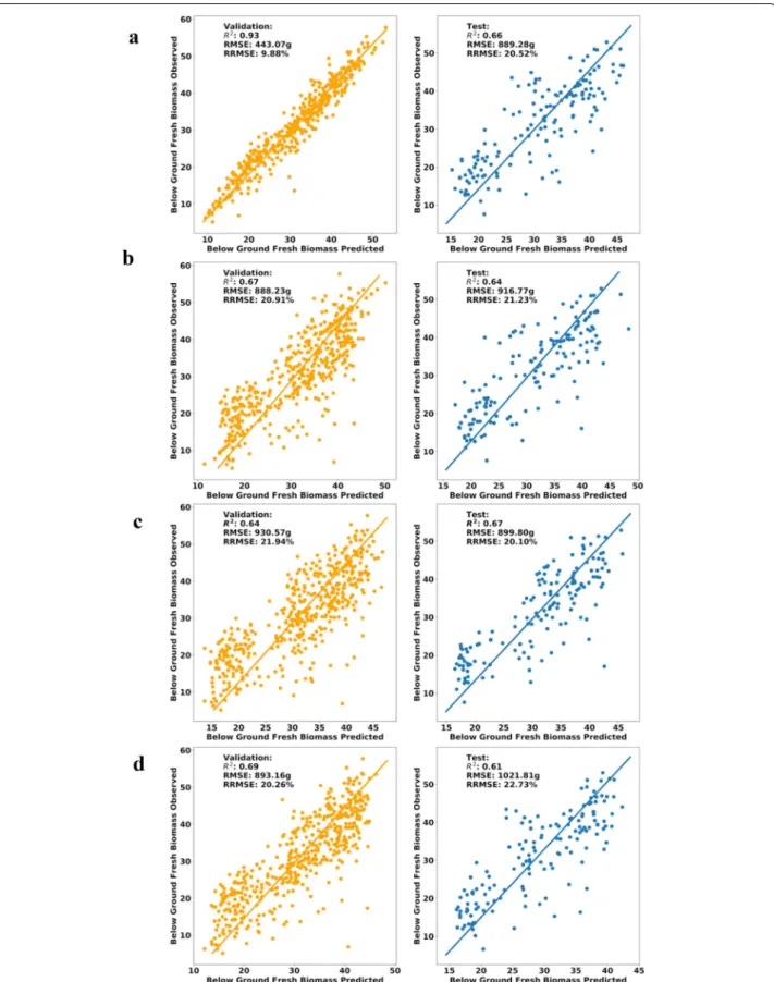
met-rics (Fig. 12). Among the four developed ML models,
the results showed consistent performance with small differences between PCA and PCR techniques ranging
from 0 to 9% along the metrics (Table 4). PCA was
per-formed little better than PCR in terms of RRMSE and R2 ranging from 20.51% to 22.73% and 0.61 to 0.67,
Fig. 11 PCA scree plot of the percent of aforementioned variance during trial two
Table 3 Total variance explained by component
Component Total variance
PC1 0.556 PC2 0.145 PC3 0.061 PC4 0.038 PC5 0.027 PC6 0.018 PC7 0.014 PC8 0.014 PC9 0.011 PC10 0.009
Fig. 12 Plots based on regression methods, validation dataset on the left and test dataset on the right. a RF parameters (max_features:4, trees: 100).
respectively. In this case, the RF model gave the most
well-adjusted results, with high R2 and lowest RMSE,
indicating the importance of VIs and canopy metrics to predict BGB by MS sensors. Even though the accuracy of developed models is not very high, considering the laborious cassava phenotyping efforts, CIAT Pheno-i will still be handy for breeders to reduce their time and efforts. This model accuracy can be easily improved by adding other features such as climate, soil, and more timing points.
Conclusions and future directions
The use of UAV platforms in rapid acquisition of pheno-typic information, such as key phenological stages and vegetation indices as described in this work, have great potential to be used as a selection tool in cassava breed-ing programs. Automated image analytical framework (CIAT Pheno-i) developed in this study showed prom-ising results and could be applied to other crops than cassava to accelerate germplasm and varietal selection. Machine learning model to predict cassava root yield using MS UAV imagery is encouraging however further validation in diverse sets of germplasm in different envi-ronments is necessary. Furthermore, the validation of this ML models in large cassava core collection is currently under progress. In summary, UAVs equipped with MS sensors rapidly monitored canopy metrics, VIs and effec-tively predicted cassava root yield in a non-destructive and cost effective way. As of now, we are also exploring other ground sensor technologies such as Ground pen-etrating radar (GPR) to predict cassava root yield more accurately by integrating above and below-ground time series information. Through different innovative remote sensing and image technologies it is highly possible to find out the hidden secrets of below-ground information in cassava which eventually bring higher accuracy in yield prediction.
Supplementary information
Supplementary information accompanies this paper at https ://doi. org/10.1186/s1300 7-020-00625 -1.
Additional file 1: Table S1. Cassava morphological and agronomic descriptors. Table S2. Phenological stage information (Months) of geno-types listed in this study. Table S3. List of hardware and software used in this study.
Additional file 2: Figure S1. Agisoft Metashape automated orthomosaic building pipeline. Figure S2. CIAT Pheno-i Front-end overview. Figure S3. Pheno-i image analysis platform design. Back-end: Developed in Python 3 and Flask as a Web Service. Front-end: Developed using React as a single page app, it implements leaflet.js to render maps. Figure S4. Schematic representation of database implemented in CIAT Pheno-i. Fig‑ ure S5. Comparison of time series data between manual and automatic orthomosaic generation with MS and RGB sensors. (a) Multispectral trial in manual mode. (b) Multispectral trial in auto mode. (c) RGB trial in manual mode. (d) RGB trial in auto mode. *M1-M8 Manual orthomosaics. *A1-A8 Automatic orthomosaics.
Additional file 3. Video of Pheno-i Image Analysis Platform (https ://youtu .be/hnq_ydC1-rw).
Abbreviations
AGB: Above-ground biomass; ANN: Artificial neural networks; API: Application program interface; BGB: Below-ground biomass; BNDVI: Blue normalized differ-ence vegetation Index; CCuav: Canopy cover estimate from UAV; CH: Canopy height; CHuav: Canopy height estimate from UAV; CIAT Pheno-i: Automated image analytical framework; CPU: Central processing unit; CSV: Comma separated values; DEM: Digital elevation model; DMA: Dry matter accumula-tion; EBK: Early bulking; EL: Elongaaccumula-tion; ELC: Empirical line calibraaccumula-tion; GNDVI: Green normalized difference vegetation index; GCPs: Ground control points; GRVI: Green-Red vegetation index; GNSS: Global navigation satellite system; GUI: Graphical user interface; GIS: Geographic information system; GMR: Green minus red; GPR: Ground penetrating radar; GDAL: Geospatial data abstraction library; HTFP: High-throughput field phenotyping; KNN: k-Nearest neighbors; LAI: Leaf area index; LBK: Late bulking; ML: Machine learning; MLP: Multi-Layer perceptron; MS: Multispectral; NIR: Near-infrared; NDRE: Normalized difference Red-Edge; NDVI: Normalized difference vegetation index; NDREI: Normalized difference Vegetation Index Red-Edge; NGBDI: Normalized Green–Blue Dif-ference Index; NPCI: Normalized pigment chlorophyll Index; CVuav: Canopy volume estimate from UAV; RTK-GPS: Real-time kinematic global positioning system; RF: Random forest; REST: Representational state transfer; IMU: Inertial measurement unit; RGB: Red, green, blue; RMSE: Root median square error; PCA: Principal component analysis; PCR: Principal component regression; RRMSE: Relative root median square error; SPA: Single page app; SVM: Support Vector Machine; UAV: Unmanned aerial vehicles; VIs: Vegetation indices; VRT: Variable rate technology.
Table 4 Root yield ML Model comparison
ML Method PCA PCR PCA vs PCR Difference (%)
R2 RMSE RRMSE R2 RMSE RRMSE R2 RMSE RRMSE
Validation RF 0.93 443.07 9.88% 0.94 449.09 9.19% 1.07% 1.35% 7.24% SVM 0.67 888.23 20.91% 0.63 947.45 22.10% 6.15% 6.45% 5.53% kNN 0.64 930.57 21.94% 0.64 953.3 22.01% 0.00% 2.41% 0.32% ANN 0.69 893.16 20.26% 0.7 910.21 21.12% 1.44% 1.89% 4.16% Test RF 0.66 889.28 20.52% 0.64 891.86 21.12% 3.08% 0.29% 2.88% SVM 0.64 916.77 21.23% 0.64 874.13 21.14% 0.00% 4.76% 0.42% kNN 0.67 899.8 20.10% 0.67 879.09 20.20% 0.00% 2.33% 0.50% ANN 0.61 1021.81 22.73% 0.61 1120.04 22.61% 0.00% 9.17% 0.53%
Acknowledgements
The authors would like to thank Hernan Ceballos, Luis Augusto Becerra, Ishitani Manabu and Joe Tohme, from the International Center for Tropical Agriculture (CIAT) for their support in this research. The authors would like to acknowledge Frank Montenegro, Alejandro Vergara, Cristhian Delgado, Jorge Casas, Sandra Salazar and all the phenomics lab members from CIAT for their support in conducting this study. As well as Angela Fernando, CIAT consultant, for her support in formatting and technical editing. Thanks to CGIAR Big Data and CGIAR Research Program on Roots, Tubers and Bananas (RTB) for their continuous encouragement to develop CIAT Pheno-i software and phenomics platform. Animesh Acharjee acknowledged support from National Institute of Health Research (NIHR) Surgical Reconstruction and Microbiology Research Centre (SRMRC). The views expressed in this publication are those of the authors and not necessarily those of the NHS, the National Institute for Health Research, the Medical Research Council or the Department of Health, UK. Author’s contributions
MGS designed the study and wrote the paper and the other authors read, edited and approved the manuscript. DG and MV helped to analyze the UAV images. MGS and MV designed the field experiments and collected the ground-truth data. MV and HR helped to develop CIAT Pheno-i Image Analysis Platform. AA guided MV to develop ML models. All authors read and approved the final manuscript.
Funding
This work was partially funded by the NSF-BREAD program through Texas A&M University.
Availability of data and materials
The data used in this study is available from the corresponding author on reasonable request.
Ethics approval and consent to participate Not applicable
Consent for publication
All authors agreed to publish this manuscript. Competing interests
The authors declare that they have no competing interests. Author details
1 International Center for Tropical Agriculture (CIAT), A.A. 6713 Cali, Colom-bia. 2 Department of Soil and Crop Sciences, Texas A&M University, College Station, TX, USA. 3 College of Medical and Dental Sciences, Institute of Cancer and Genomic Sciences, Centre for Computational Biology, University of Bir-mingham, Birmingham B15 2TT, UK. 4 Institute of Translational Medicine, Uni-versity Hospitals Birmingham NHS Foundation Trust, Birmingham B15 2TT, UK. 5 NIHR Surgical Reconstruction and Microbiology Research Centre, University Hospital Birmingham, Birmingham B15 2WB, UK.
Received: 19 February 2020 Accepted: 28 May 2020
References
1. Allem AC, Mendes RA, Salomão AN, Burle ML. The primary gene pool of cassava (Manihot esculenta Crantz subspecies esculenta, Euphorbiaceae). In: Euphytica. Springer Netherlands; 2001. p. 127–32.
2. Oyewole O, Africa SO-J of FT in, 2001 undefined. Effect of length of fermentation on the functional characteristics of fermented cassava’fufu’. ajol.info. https ://www.ajol.info/index .php/jfta/artic le/view/19283 . Accessed 20 Jan 2020.
3. Pearce F. Cassava comeback. New Sci. 2007;194(2600):38–9. 4. Malik AI, Kongsil P, Nguyen VA, Ou W, Sholihin, Srean P, et al. Cassava
breeding and agronomy in Asia—50 years of history and future direc-tions. Breed Sci (Accept MS); 2020.
5. Lynam J, Byerlee D. Forever Pioneers: CIAT: 50 Years Contributing to a sus-tainable food future and counting. CIAT. Vol. 2009, Cali, Colombia; 2017.
https ://cgspa ce.cgiar .org/bitst ream/handl e/10568 /89043 /CIAT5 0_FOREV ER_PIONE ERS.pdf?seque nce=3. Accessed 20 Jan 2020.
6. Walter J, Edwards J, Cai J, McDonald G, Miklavcic SJ, Kuchel H. High-Throughput field imaging and basic image analysis in a wheat breeding programme. Front Plant Sci. 2019:10. https ://www.front iersi n.org/artic le/10.3389/fpls.2019.00449 /full. Accessed 21 Jan 2020.
7. Qiu Q, Sun N, Bai H, Wang N, Fan Z, Wang Y, et al. Field-based high-throughput phenotyping for maize plant using 3d LIDAR point cloud generated with a “phenomobile”. Front Plant Sci. 2019;16:10.
8. Delgado A, Hays DB, Bruton RK, Ceballos H, Novo A, Boi E, et al. Ground penetrating radar: a case study for estimating root bulking rate in cas-sava (Manihot esculenta Crantz). Plant Methods. 2017;13(1):65. http:// plant metho ds.biome dcent ral.com/artic les/10.1186/s1300 7-017-0216-0. Accessed 20 Jan 2020.
9. Ceballos H, Pérez JC, Joaqui Barandica O, Lenis JI, Morante N, Calle F, et al. Cassava breeding I: the value of breeding value. Front Plant Sci. 2016;7. http://journ al.front iersi n.org/Artic le/10.3389/fpls.2016.01227 /abstr act. Accessed 21 Jan 2020.
10. Nduwumuremyi A, Melis R, Shanahan P, Theodore A. Analysis of pheno-typic variability for yield and quality traits within a collection of cassava (Manihot esculenta) genotypes. South Afr J Plant Soil. 2018;35(3):199–206. 11. Selvaraj MG, Montoya-P ME, Atanbori J, French AP, Pridmore T. A low-cost aeroponic phenotyping system for storage root development: unravel-ling the below-ground secrets of cassava (Manihot esculenta). Plant Methods. 2019;15:131.
12. Atanbori J, Montoya-P ME, Selvaraj MG, French AP, Pridmore TP. Convo-lutional neural net-based cassava storage root counting using real and synthetic images. Front Plant Sci. 2019;10. https ://www.front iersi n.org/ artic le/10.3389/fpls.2019.01516 /full. Accessed 21 Jan 2020.
13. Vitor AB, Diniz RP, Morgante CV, Antônio RP, de Oliveira EJ. Early predic-tion models for cassava root yield in different water regimes. F Crop Res. 2019;1(239):149–58.
14. Zhao C, Zhang Y, Du J, Guo X, Wen W, Gu S, et al. Crop phenomics: current status and perspectives. Front Plant Sci. 2019;10:714.
15. Haghighattalab A, González Pérez L, Mondal S, Singh D, Schinstock D, Rutkoski J, et al. Application of unmanned aerial systems for high throughput phenotyping of large wheat breeding nurseries. Plant Methods. 2016;12:35. http://www.plann er.ardup ilot.com. Accessed 21 Jan 2020.
16. Delgado A, Novo A, Hays DB. Data Acquisition Methodologies Utilizing Ground Penetrating Radar for Cassava (Manihot esculenta Crantz) Root Architecture. Geosciences. 2019;9(4):171. https ://www.mdpi.com/2076-3263/9/4/171. Accessed 21 Jan 2020.
17. Quirós Vargas JJ, Zhang C, Smitchger JA, McGee RJ, Sankaran S. Pheno-typing of plant biomass and performance traits using remote sensing techniques in pea (Pisum sativum, L.). Sensors. 2019;19(9):2031. https :// www.mdpi.com/1424-8220/19/9/2031. Accessed 21 Jan 2020. 18. Jay S, Baret F, Dutartre D, Malatesta G, Héno S, Comar A, et al.
Exploit-ing the centimeter resolution of UAV multispectral imagery to improve remote-sensing estimates of canopy structure and biochemistry in sugar beet crops. Remote Sens Environ. 2019;15:231.
19. Furbank RT, Jimenez‐Berni JA, George‐Jaeggli B, Potgieter AB, Deery DM. Field crop phenomics: enabling breeding for radiation use efficiency and biomass in cereal crops. New Phytol. 2019;223(4):1714–27. https ://onlin elibr ary.wiley .com/doi/abs/10.1111/nph.15817 . Accessed 21 Jan 2020. 20. Hassan MA, Yang M, Rasheed A, Yang G, Reynolds M, Xia X, et al. A rapid
monitoring of NDVI across the wheat growth cycle for grain yield predic-tion using a multi-spectral UAV platform. Plant Sci. 2019;1(282):95–103. 21. Pantazi XE, Moshou D, Alexandridis T, Whetton RL, Mouazen AM. Wheat
yield prediction using machine learning and advanced sensing tech-niques. Comput Electron Agric. 2016;1(121):57–65.
22. Everingham Y, Sexton J, Skocaj D, Inman-Bamber G. Accurate prediction of sugarcane yield using a random forest algorithm. Agron Sustain Dev. 2016;36:27.
23. Chlingaryan A, Sukkarieh S, Whelan B. Machine learning approaches for crop yield prediction and nitrogen status estimation in precision agricul-ture: a review. Comput Electron Agric. 2018;151:61–9.
24. Jeffries GR, Griffin TS, Fleisher DH, Naumova EN, Koch M, Wardlow BD. Mapping sub-field maize yields in Nebraska, USA by combining remote sensing imagery, crop simulation models, and machine learning. Precis Agric. 2019;21:678.
25. Kamir E, Waldner F, Hochman Z. Estimating wheat yields in Australia using climate records, satellite image time series and machine learning methods. ISPRS J Photogramm Remote Sens. 2020;1(160):124–35. 26. Li J, Veeranampalayam-Sivakumar AN, Bhatta M, Garst ND, Stoll H,
Stephen Baenziger P, et al. Principal variable selection to explain grain yield variation in winter wheat from features extracted from UAV imagery. Plant Methods. 2019;15:123.
27. Zhou X, Zheng HB, Xu XQ, He JY, Ge XK, Yao X, et al. Predicting grain yield in rice using multi-temporal vegetation indices from UAV-based multispectral and digital imagery. ISPRS J Photogramm Remote Sens. 2017;130:246–55. https ://doi.org/10.1016/j.isprs jprs.2017.05.003. 28. Naik HS, Zhang J, Lofquist A, Assefa T, Sarkar S, Ackerman D, et al. A
real-time phenotyping framework using machine learning for plant stress severity rating in soybean. Plant Methods. 2017;13(1):23. http:// plant metho ds.biome dcent ral.com/artic les/10.1186/s1300 7-017-0173-7. Accessed 21 Jan 2020.
29. Cen H, Wan L, Zhu J, Li Y, Li X, Zhu Y, et al. Dynamic monitoring of biomass of rice under different nitrogen treatments using a lightweight UAV with dual image-frame snapshot cameras. Plant Methods. 2019;15:32. 30. Han L, Yang G, Dai H, Xu B, Yang H, Feng H, et al. Modeling maize
above-ground biomass based on machine learning approaches using UAV remote-sensing data. Plant Methods. 2019;15:10.
31. Zahid A, Abbas HT, Ren A, Zoha A, Heidari H, Shah SA, et al. Machine learning driven non - invasive approach of water content estimation in living plant leaves using terahertz waves. Plant Methods. 2019. https :// doi.org/10.1186/s1300 7-019-0522-9.
32. Roitsch T, Cabrera-Bosquet L, Fournier A, Ghamkhar K, Jiménez-Berni J, Pinto F, et al. Review: new sensors and data-driven approaches—a path to next generation phenomics. Plant Sci. 2019;282:2–10.
33. Fiorani F, Schurr U. Future scenarios for plant phenotyping. Annu Rev Plant Biol. 2013;64(1):267–91. http://www.annua lrevi ews.org/ doi/10.1146/annur ev-arpla nt-05031 2-12013 7. Accessed 21 Jan 2020. 34. Czedik-Eysenberg A, Seitner S, Güldener U, Koemeda S, Jez J, Colombini
M, et al. The ‘PhenoBox’, a flexible, automated, open-source plant pheno-typing solution. New Phytol. 2018;219(2):808–23.
35. Xue J, Su B. Significant remote sensing vegetation indices: a review of developments and applications. hindawi.com; 2017. https ://doi. org/10.1155/2017/13536 91. Accessed 2 Apr 2020.
36. Fukuda WMG, Guevara CL, Kawuki R, Ferguson ME. Selected morphologi-cal and agronomic descriptors for the characterization of cassava. https :// www.iita.org. Accessed 21 Jan 2020.
37. LI-2200C Plant Canopy Analyzer. https ://www.licor .com/env/produ cts/ leaf_area/LAI-2200C /. Accessed 31 Mar 2020.
38. Barnes E, Clarke T, Richards S, Colaizzi P, Haberland J, Kostrzewski M, et al. Coincident detection of crop water stress, nitrogen status and canopy density using ground-based multispectral data; 2000.
39. Tucker CJ. Red and photographic infrared linear combinations for moni-toring vegetation. Remote Sens Environ. 1979;8:2.
40. Moges SM, Raun WR, Mullen RW, Freeman KW, Johnson G V., Solie JB. Evaluation of green, red, and near infrared bands for predicting winter wheat biomass, nitrogen uptake, and final grain yield. J Plant Nutr. 2005;27(8):1431–41. http://www.tandf onlin e.com/doi/abs/10.1081/PLN-20002 5858. Accessed 10 Feb 2020.
41. Wang F, Huang J, Tang Y, Wang X. New vegetation index and its applica-tion in estimating leaf area index of rice. Rice Sci. 2007;14(3):195–203. 42. Gitelson A, Merzlyak MN. Quantitative estimation of chlorophyll-a using
reflectance spectra: experiments with autumn chestnut and maple leaves. J Photochem Photobiol B Biol. 1994;22(3):247–52.
43. Peñuelas J, Gamon JA, Fredeen AL, Merino J, Field CB. Reflectance indices associated with physiological changes in nitrogen- and water-limited sunflower leaves. Remote Sens Environ. 1994;48(2):135–46. 44. Wang Y, Wang D, Zhang G, Wang J. Estimating nitrogen status of rice
using the image segmentation of G-R thresholding method. F Crop Res. 2013;1(149):33–9.
45. Otsu N. A threshold selection method from gray-level histograms. IEEE Trans Syst Man Cybern. 1979;9(1):62–6.
46. Kuhn M, Johnson K. Applied predictive modeling. Applied predictive modeling. New York: Springer; 2013. p. 1–600.
47. Jolliffe IT. A note on the use of principal components in regression. Appl Stat. 1982;31(3):300. https ://www.jstor .org/stabl e/10.2307/23480 05?origi n=cross ref. Accessed 3 Apr 2020.
48. Gago J, Fernie AR, Nikoloski Z, Tohge T, Martorell S, Escalona JM, et al. Integrative field scale phenotyping for investigating metabolic compo-nents of water stress within a vineyard. Plant Methods. 2017;13:90. 49. Nagasubramanian K, Jones S, Sarkar S, Singh AK, Singh A,
Ganapathysub-ramanian B. Hyperspectral band selection using genetic algorithm and support vector machines for early identification of charcoal rot disease in soybean stems. Plant Methods. 2018;14:86.
50. Schirrmann M, Giebel A, Gleiniger F, Pflanz M, Lentschke J, Dammer K-H. Monitoring agronomic parameters of winter wheat crops with low-cost UAV imagery. Remote Sens. 2016;8(9):706. http://www.mdpi.com/2072-4292/8/9/706. Accessed 21 Jan 2020.
51. Albon C. Machine learning with python cookbook: Practical solutions from preprocessing to deep learning; 2018. https ://books .googl e.com/ books ?hl=en&lr=&id=kIhQD wAAQB AJ&oi=fnd&pg=PT80&dq=Machi ne+learn ing+with+pytho n+cookb ook:+Pract ical+solut
ions+from+prepr ocess ing+to+deep+learn ing&ots=OmYqZ HgnKR &sig=yWJeX Crjii 9Nd4g WcnrC zAj1T uc. Accessed 12 Feb 2020.
52. Ho TK. Random decision forests. In: Proceedings of the International Con-ference on Document Analysis and Recognition, ICDAR. IEEE Computer Society; 1995. p. 278–82.
53. Cortes C, Vapnik V. Support-vector networks. Mach Learn. 1995;20(3):273–97.
54. Altman NS. An introduction to kernel and nearest-neighbor nonparamet-ric regression. Am Stat. 1992;46(3):175–85.
55. Nair V, Hinton GE. Rectified linear units improve restricted boltzmann machines.https ://www.cs.toron to.edu/~hinto n/absps /reluI CML.pdf.. Accessed 15 Jan 2020.
56. Minervini M, Giuffrida MV, Perata P, Tsaftaris SA. Phenotiki: an open software and hardware platform for affordable and easy image-based phenotyping of rosette-shaped plants. Plant J. 2017;90(1):204–16. https :// doi.org/10.1111/tpj.13472 .
57. Gago J, Douthe C, Coopman RE, Gallego PP, Ribas-Carbo M, Flexas J, et al. UAVs challenge to assess water stress for sustainable agriculture. Agric Water Manage. 2015;153:9–19.
58. Sankaran S, Khot LR, Espinoza CZ, Jarolmasjed S, Sathuvalli VR, Vandemark GJ, et al. Low-altitude, high-resolution aerial imaging systems for row and field crop phenotyping: a review. Eur J Agron. 2015;70:112–23.
59. van der Meij B, Kooistra L, Suomalainen J, Barel JM, De Deyn GB. Remote sensing of plant trait responses to field-based plant–soil feedback using UAV-based optical sensors. Biogeosciences. 2017;14(3):733–49. https :// www.bioge oscie nces.net/14/733/2017/. Accessed 22 Jan 2020. 60. Araus JL, Cairns JE. Field high-throughput phenotyping: the new crop
breeding frontier. Trends Plant Sci. 2014;19:52–61.
61. Zaman-Allah M, Vergara O, Araus JL, Tarekegne A, Magorokosho C, Zarco-Tejada PJ, et al. Unmanned aerial platform-based multi-spectral imaging for field phenotyping of maize. Plant Methods. 2015;11:35.
62. Aasen H, Burkart A, Bolten A, Bareth G. Generating 3D hyperspectral infor-mation with lightweight UAV snapshot cameras for vegetation monitor-ing: from camera calibration to quality assurance. ISPRS J Photogramm Remote Sens. 2015;1(108):245–59.
63. Domingues Franceschini M, Bartholomeus H, van Apeldoorn D, Suoma-lainen J, Kooistra L. Intercomparison of unmanned aerial vehicle and ground-based narrow band spectrometers applied to crop trait monitor-ing in organic potato production. Sensors. 2017;17(6):1428. http://www. mdpi.com/1424-8220/17/6/1428. Accessed 22 Jan 2020.
64. Jin X, Liu S, Baret F, Hemerlé M, Comar A. Estimates of plant density of wheat crops at emergence from very low altitude UAV imagery. Remote Sens Environ. 2017;1(198):105–14.
65. Duan B, Fang S, Zhu R, Wu X, Wang S, Gong Y, et al. Remote estimation of rice yield with unmanned aerial vehicle (uav) data and spectral mixture analysis. Front Plant Sci. 2019;7:10.
66. Singh D, Wang X, Kumar U, Gao L, Noor M, Imtiaz M, et al. High-Through-put phenotyping enabled genetic dissection of crop lodging in wheat. Front Plant Sci. 2019;10. https ://www.front iersi n.org/artic le/10.3389/ fpls.2019.00394 /full. Accessed 22 Jan 2020.
67. Shafian S, Rajan N, Schnell R, Bagavathiannan M, Valasek J, Shi Y, et al. Unmanned aerial systems-based remote sensing for monitoring sor-ghum growth and development. PLoS ONE. 2018;13:5.
68. Okogbenin E, Setter TL, Ferguson M, Mutegi R, Ceballos H, Olasanmi B, et al. Phenotypic approaches to drought in cassava: review. Front Physiol. 2013;4:93.