Distance Learning and Attribute Importance Analysis by Linear Regression on Idealized Distance Functions

(1)

Wright State University

CORE Scholar

Browse all Theses and Dissertations

Theses and Dissertations

2017

Distance Learning and Attribute Importance Analysis by Linear

Regression on Idealized Distance Functions

Rupesh Kumar Singh

Wright State University

Follow this and additional works at: https://corescholar.libraries.wright.edu/etd_all Part of the Computer Engineering Commons, and the Computer Sciences Commons

Repository Citation

Singh, Rupesh Kumar, "Distance Learning and Attribute Importance Analysis by Linear Regression on Idealized Distance Functions" (2017). Browse all Theses and Dissertations. 1739.

https://corescholar.libraries.wright.edu/etd_all/1739

This Thesis is brought to you for free and open access by the Theses and Dissertations at CORE Scholar. It has been accepted for inclusion in Browse all Theses and Dissertations by an authorized administrator of CORE Scholar. For more information, please contact library-corescholar@wright.edu.

(2)

DISTANCE LEARNING AND

ATTRIBUTE IMPORTANCE

ANALYSIS BY LINEAR

REGRESSION ON IDEALIZED

DISTANCE FUNCTIONS

A thesis submitted in partial fulfillment of the requirements for the degree of Masters of Science in Computer Engineering

By

RUPESH KUMAR SINGH

B.E., Electronics and Communication Engineering, Tribhuvan University, 2014

2017

(3)

WRIGHT STATE UNIVERSITY GRADUATE SCHOOL

May 16, 2017 I HEREBY RECOMMEND THAT THE THESIS PREPARED UNDER MY SUPERVISION BY Rupesh Kumar SinghENTITLEDDistance Learning and Attribute Importance Analysis by Linear Regression on Idealized Distance Functions BE ACCEPTED IN PARTIAL FUL-FILLMENT OF THE REQUIREMENTS FOR THE DEGREE OFMasters of Science in Computer Engineering.

Guozhu Dong, Ph.D. Thesis Director

Mateen M. Rizki, Ph.D.

Chair, Department of Computer Science and Engineering Committee on Final Examination Guozhu Dong, Ph.D. Keke Chen, Ph.D. Michelle Cheatham, Ph.D. Robert E. W. Fyffe, Ph.D.

Vice President for Research and Dean of the Graduate School

(4)

ABSTRACT

Singh, Rupesh Kumar. MSCE, Department of Computer Science and Engineering, Wright State University, 2017. Distance Learning and Attribute Importance Analysis by Linear Regression on Idealized Distance Functions.

A good distance metric is instrumental on the performance of many tasks including classification and data retrieval. However, designing an optimal distance function is very challenging, especially when the data has high dimensions. Recently, a number of algorithms have been proposed to learn an optimal distance function in a supervised manner, using data with class labels. In this thesis we proposed methods to learn an optimal distance function that can also indicate the importance of attributes.

Specifically, we present several ways to define idealized distance functions, two of which involving distance error correction involving KNN classification, and another involving a two-constant defined distance function. Then we use multiple linear regression to produce regression formulas to represent the idealized distance functions. Experiments indicate that distances produced by our approaches have classification accuracy that are fairly comparable to existing methods. Importantly, our meth-ods have added bonus of using weights on attributes to indicate the importance of attributes in the constructed optimal distance functions.

Finally, the thesis presents importance of attributes on a number of datasets from the UCI repository.

Keywords: Distance learning; move bad neighbors out; global class gap; two-constant distance; weighted distance function; Euclidean; Manhattan

(5)

List of Figures

2.1 Example for KNN . . . 4

2.2 Basic example of linear regression . . . 5

3.1 Using Ideal Distance to get Weighted Distance Function . . . 8

3.2 Illustration of WeightedL1norm . . . 9

3.3 Error correction Based Approach . . . 11

3.4 Illustration of Move Bad Neighbors Out Method . . . 12

(8)

List of Tables

4.1 Summary of the datasets . . . 17 4.2 Part 1 - KNN classification accuracy of 5 different algorithms: Manhattan as Manh,

Euclidean as Euc, DL(L1,GCG) denoted by L1GCG, DL(L1,MBNO) denoted by

L1MBNO and DL(L2,GCG) denoted by L2GCG . . . 18

4.3 Part 2 - KNN classification accuracy of 5 different algorithms: DL(L2,MBNO)

de-noted by L2MBNO, DL2C(L1) denoted by 2CL1, DL2C(L1,MBNO) denoted by

2CL1MBNO, DL2C(L2,MBNO) denoted by 2CL2MBNO and DL2C(L2) denoted by

2CL2 . . . 18 4.4 Part 1 - KNN classification accuracy of 5 different algorithms: Manhattan as Manh,

L1MBNO and DL(L2,GCG) denoted by L2GCG . . . 19

4.5 Part 2 - KNN classification accuracy of 5 different algorithms: DL(L2,MBNO)

de-noted by L2MBNO, DL2C(L1) denoted by 2CL1, DL2C(L1,MBNO) denoted by

2CL1MBNO, DL2C(L2,MBNO) denoted by 2CL2MBNO and DL2C(L2) denoted by

2CL2 . . . 19 4.6 Classification accuracy of 5 different algorithms: DL2C(L1,MBNO) denoted by 2CL1MBNO,

DL(L1,GCG) denoted by L1GCG, Large Margin Nearest Neighbor (LMNN),

Information-Theoretic Metric Learning (ITML) and Support Vector Machine (SVM) . . . 23 4.7 Top 2 positive big change attributes and top 2 negative big change attributes . . . . 24 4.8 Impact of different values ofγ on GCG . . . 25 4.9 Impact of different values ofν on MBNO . . . 26 4.10 Part 1 - KNN classification accuracy of 6 different algorithms: Manhattan as Manh,

L1MBNO, DL(L2,MBNO) denoted by L2MBNO and DL(L2,GCG) denoted by L2GCG

. . . 27

(9)

4.11 Part 2 - KNN classification accuracy of 6 different algorithms: DL2C(L1) denoted

by 2CL1, DL2C(L1,MBNO) denoted by 2CL1MBNO, DL2C(L1,GCG) denoted by

2CL1GCG, DL2C(L2,GCG) denoted by 2CL2GCG, DL2C(L2,MBNO) denoted by

2CL2MBNO and DL2C(L2) denoted by 2CL2 . . . 28

(10)

ACKNOWLEDGEMENTS

I am very grateful to a lot of people who have supported and guided me throughout my life. I would like to thank my advisor Dr. Guozhu Dong for his motivational advising skills and his guidance and support during my thesis. I am grateful to Dr. Dong for his door was always open whenever i ran into a problem related to thesis writing or any concept/algorithm. He consistently steered me in the right directions giving valuable vision on establishing my career and addressing real-world problems. He is one of the best mentor i ever had.

I would also like to thank my committee members, Dr. Keke Chen and Dr. Michelle Cheatham for their support ,guidance and productive comments towards the completion of this thesis.

I would also like to thank my family for all the sacrifices they have made on my behalf throughout my life. I could never find enough words to express their support and guidance.

And finally, last but by no means least, i would like to thank my colleagues at Kno.e.sis Center and Wright State University for their support and guidance throughout my thesis.

Thank you.

(11)

1

Introduction

A good distance metric in high dimensional space is crucial for the real-world applications. Most of the machine learning algorithms relying on a distance metric can be improved strikingly by learning a good distance metric. For example, we want to classify images of faces by age and facial expression based on class labels. The same distance function cannot be ideal for both the classifications even though attributes for both the classifications remain same. So, a good distance metric plays an important role in classification. For example, KNN (k-nearest neighbors) [Cover and Hart 1967], is one of the widely used simple and effective algorithm for classification. It is a non-parametric and supervised classification algorithm that employs class labels of training data to determine the class of an unseen instance. Some research studies [Chopra et al. 2005] [Hastie and Tibshirani 1995] have shown that KNN performance can be improved notably by learning a good distance metric. We also used KNN to evaluate and test the accuracy of our weighted distance metric.

A number of research studies [Goldberger et al. 2004] [Tsang et al. 2003] [Weinberger et al. 2005] [Xing et al. 2002] [Shalev-Shwartz et al. 2004] [Schultz and Joachims 2003] have shown that a good distance metric can boost the performance of distant based algorithms. KNN and other distance based algorithms often implement Euclidean to measure distance between two instances. To some extent Euclidean distance metric works fine but with higher number of attributes it fails to mea-sure the statistical regularities or underlying data distribution that might be present in the training dataset. Along with it, Euclidean and Manhattan distance functions give equal weight of one to every attribute present in the dataset and hence, they mislead the distance based on weight. Since

(12)

2 most of the datasets nowadays have multiple attributes, the distance is dominated by the irrelevant attributes present giving inaccurate results while employing Euclidean or Manhattan distance func-tions. Here, in this thesis, we focus on choosing improved distance functions which can be applied to almost all the distance based learning algorithms.

This thesis presents a novel method which develops idealized distance function and then uses linear regression to determine weights for weighted Euclidean and weighted Manhattan distance func-tions. Idealized distance is calculated based on two approach: error correction and Two-constant. We have two approach named as: Global Class Gap (GCG) and Move Bad Neighbors Out (MBNO) to accomplish our achievements for computation of idealized distance function through error correc-tion.

In Chapter 3, we describe our error correction methods, Two-constant approach and distance metric learning algorithms. In Chapter 4, we compare performance among our different methods and also compared performance of our two winners methods with other popular methods. Along with it, we give some insights on attribute importance and describe impacts of different parameters on our methods.

(13)

2

Preliminaries

Before we describe our approach and experimentation results, we briefly explain some basic termi-nology that will guide us to understand our algorithms. This part introduces basic concepts related to following topics.

• KNN

• Distance metric

• Linear regression

2.1

Distance Metric

There are different distance metrics used in the machine learning algorithms and in this thesis, we are going to use Euclidean and Manhattan.

Euclidean distance metric is also known as L2 norm. Euclidean distance between points X and Z is defined as: f(X, Z) = v u u t n X i=1 (xi−zi)2

whereX = (x1, ..., xn), Z= (z1, ..., zn) and n is number of attributes.

Manhattan distance metric is also known as rectilinear distance orL1norm. Manhattan distance between points X and Z is defined as:

f(X, Z) = n X

i=1

|xi−zi|

whereX = (x1, ..., xn), Z= (z1, ..., zn) and n is number of attributes.

(14)

2.2. KNN 4 The above mentioned distance metrics are used to measure similarities or differences between two tuples based on distance. We will use the metrics to estimate weights for weighted Manhattan and weighted Euclidean distance functions.

2.2

KNN

KNN [Cover and Hart 1967] is a supervised classification algorithm which uses closest k training instances to determine class of a test instance. It defines the class of the test instance based on the similarities measure by distance functions.

The test instance is classified by majority vote of its k closest neighbors such that the instance being assigned to the most common class within its k nearest neighbors.

LetX1, X2, .., Xtbe t training instances withnattributes andZbe a test instance whose class is to be determined. Distances between Z and all the training instances are calculated using Manhattan or Euclidean distance metric.

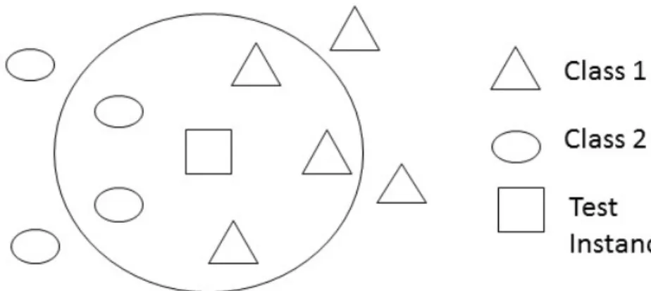
If we sort neighbors of Z based on distance then k nearest training instances determine class of Z based on the majority votes. In the given Figure 2.1, 5 (k=5) nearest neighbors are chosen to determine class of the test instance. Since, there are two Class 2 instances and three Class 1 instances, the test instance falls under Class 1 by the majority votes.

So, how is KNN going to help in our distance metric learning? Idealized distance in our approach is computed based on KNN such that the k closest neighbors whose presence leads to error is corrected by moving the neighbors to some distant away. It is also used to evaluate and test classification

(15)

2.3. REGRESSION 5 accuracy of our methods.

2.3

Regression

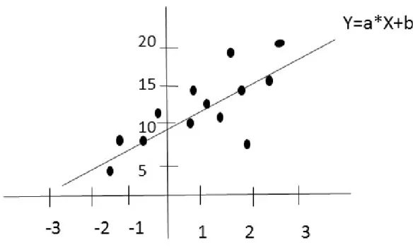
Figure 2.2: Basic example of linear regression

Regression analysis is a statistical method that models and analyzes the relationship between dependent variable (also called response) and a series of independent variables (also known as predictors). It is often used in finance, weather and other disciplines that uses prediction and forecasting.

There are many types of regression and linear regression is one of them. The regression with one independent variable is known as simple linear regression whereas the regression with more than one independent variables is known as multiple linear regression. In this thesis, we are going to use multiple linear regression for our distance metric learning. Linear regression helps to understand and examine how the value of dependent variable related to independent variable and which independent variable plays a significant role in predicting dependent variable.

(16)

2.3. REGRESSION 6 a baseline equation given asy=a∗x+b, where x is independent variable, y is dependent variable, a is regression coefficient (the slope of the line) and b is the intercept.

So, how is linear regression going to help in our distance function? Linear regression helps to derive relationship between distance and the attributes. More importantly, it helps to give some insights on the importance of attributes.

(17)

3

Our Methods

In this chapter, we describe our error correction methods, the Two-constant approach and algo-rithms.

Weighted distance function helps us to know the importance of each attribute by assigning cer-tain weight to it. Higher weight will contribute more towards distance function and lower weight will contribute lesser while zero weight has no significance in distance calculation. So, automated weight calculation of attributes plays vital role in the distance metric learning.

Our main framework is to develop idealized distance functions and then use linear regression to estimate weights for weighted Euclidean or weighted Manhattan distance functions. Applying linear regression on the idealized distance gives a better framework for the distance metric learning with improved distance function.

In our methods, we compute idealized distance based on three methods: 1) MBNO, 2) GCG and 3) the Two constant approach (dist2C). MBNO takes KNN as the measure for ideal distance computation. Since KNN classifies a test instance based on majority votes of thekclosest training instances, we give a true class label to the test instance by moving closest instances with different class labels to some distance away. The computation of ideal distance by GCG is quite different from MBNO: it aims at bringing same class instances closer and different class instances farther. The Two-constant method computes ideal distance with a novel method where it defines the distance of same class instances to be smaller than different class instances.

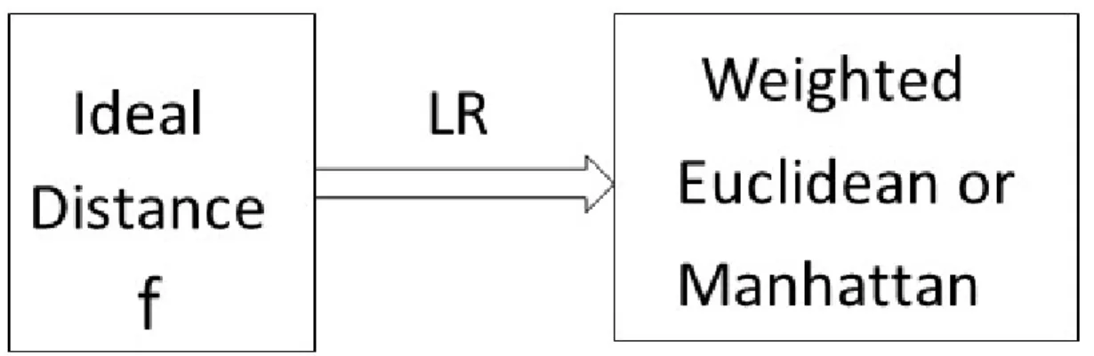
Figure 3.1represents the basic framework of our method where LR is linear regression. Linear regression is used to estimate weight of attributes for weighted Euclidean or weighted Manhattan from the ideal distance computed by MBNO, GCG or the Two-constant method.

(18)

3.1. USING REGRESSION TO REPRESENT DISTANCE FUNCTIONS 8

Figure 3.1: Using Ideal Distance to get Weighted Distance Function

3.1

Using regression to represent distance functions

Using regression to represent distance functions helps to approximate importance of each attribute in computation of weighted distance function. To model an approximation of a distance function, a training dataset for regression is required (representing a given distance functionf) which is used by linear regression to produce an approximate distance function off.

This approximation is needed since the original distance functionf may only be defined on the training data, and cannot be applied to testing data directly. Using linear regression, we produce an approximation off which can be applied to testing data directly.

Given a training datasetD, a distance function f, training dataset for linear regression is given as:

{(|x1−z1|i, ...,|xd−zd|i, f(X, Z))|X, Z∈D, X6=Z, X= (x1, ..., xd), Z= (z1, ..., zd),i∈ {1,2}}

In regression modeling terminology, the firstdcolumns, namely|x1−z1|i, ...,|xd−zd|i, are the predictor (or input) variables, and the last column, namely f(X, Z), is the response (or output) variable.

It is not easy to assign weight to each attribute of the dataset manually which will give some better distance function. So, assigning weight to each attribute automatically is an important part of weighted distance metric learning.

(19)

3.1. USING REGRESSION TO REPRESENT DISTANCE FUNCTIONS 9 Linear regression models a function which estimates weight for each attribute based on the training dataset. The weighted distance function modeled by linear regression is defined as below: A weighted distance normf is given as

f(X, Z) = n X d=1 wd|xd−zd|i !1/i

whereX = (x1, ..., xn), Z= (z1, ..., zn), wdis the weight ofdthattribute,i∈ {1,2}

The weighted distance function assigns weight to each attribute of a dataset based on idealized distance. The weight of an attribute is a real number which means that the attribute can have positive, negative or zero weight.

Figure 3.2: Illustration of WeightedL1 norm

Figure3.2illustrates an example for weightedL1norm. In the given figure, A depicts an example ofL1norm where weight of each attribute is 1. Distances among 4 data points based on the distance function 10 +|X2−X1|+|Y2−Y1|is shown in the figure. Similarly, B is an example for weighted distance function, 10 +|X2−X1| −2|Y2−Y1|, where weight of second attribute is -2 and weight of first attribute is 1. As we can see in the figure, second attribute plays vital role in determining the distance between points.

As discussed earlier, negative weight tends to bring data points closer and the given Figure3.2is an example. If we compare distance between A and B, we can see that there are changes in distances. (9,9) and (9,5) have distance of 14 in A and 2 in B. Similarly (6,8) and (6,5) have distance of 13

(20)

3.2. GETTING IDEALIZED DISTANCE BY ERROR CORRECTION (EC) 10 in A and 4 in B. If we compare these two pairs of points, we can see that the difference in second attribute for (9,9) and (9,5) is 4 and for (6,8) and (6,5) is 3. The weighted distance is highly influenced by the change in attributes. So, greater the change in attributes with negative weight, more closer will be the data points. So, pair of points (9,9) and (9,5) is closer (or has smallest distance) in B though having largest distance in A. Distance between pair of points (6,5) and (9,5) remains same in both A and B, and the reason is that the second attribute does not change. So, the influence of change in second attribute cannot be seen and the distance remains same.

The change in corresponding attributes directly influence the weighted distance based on the weight of the attributes. The characteristic of positive, negative and zero weights are described below:

• Positive weight: It adds to the total distance increasing the distance between data points.

• Zero weight: It will nullify the effect of an attribute on distance computation which means that the weighted distance value is as if there was no such attribute in the dataset.

• Negative weight: It deducts to the total distance bringing the data points closer.

3.2

Getting idealized distance by error correction (EC)

In this section, we describe the concepts and algorithms for error correction. Error correction is performed on instances to get the idealized distance which can be used by linear regression to model a weighted distance function. We describe two algorithms for error correction named as: 1) MBNO and 2) GCG.

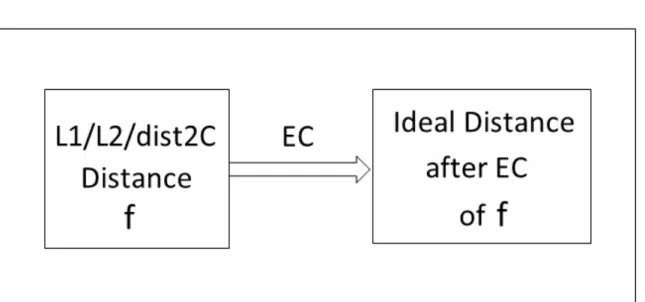
MBNO computes ideal distance based on KNN classification whereas GCG, on the other hand, assumes that minimum distance of different class tuples should be larger than maximum distance of same class tuples. The error correction method is illustrated in Figure3.3. As shown in Figure 3.3, EC is error correction method and can be applied toL1norm,L2norm or the Two-constant (dist2C) approach giving ideal distance.

These two methods are described below and are used for error correction while performing experiments.

(21)

3.2. GETTING IDEALIZED DISTANCE BY ERROR CORRECTION (EC) 11

Figure 3.3: Error correction Based Approach

3.2.1

Move Bad Neighbors Out (MBNO)

MBNO computes ideal distance based on KNN classification by modifying the distance whose pres-ence leads to error. The instance leading to error is moved to some distance away where it’s prespres-ence has no impact on KNN classification for that specific instance.

Since this method computes ideal distance for each two instances by KNN procedure, it may be called as ”Local” method. This technique will improve the KNN classification accuracy and hence provide linear regression with the ideal training dataset for approximating new distance function.

MBNO has two parameters: kfor use in KNN classification, andνfor specifying how far to move bad neighbors out.

For MBNO, error correction is performed in relation with KNN classification. The main idea is to move bad neighbors, whose presence leads to errors in KNN classification, out of the neighborhoods (that impacting KNN) by modifying certain distances. This correction modifies the given distance function differently, depending on the class distribution of data points in the neighborhood. This error correction has the potential to improve the KNN classification accuracy and hence the quality of the distance function.

LetD denote the training data with classes andf the given distance function. Letf0_{denote the}

resulting distance function after error correction.

For each X∈D, letNk(X, D, f) denote the set of theknearest neighbors ofX in D under the distance functionf. A tuple W in D is abad neighbor ofX ifW is inNk(X, D, f) andX and W

(22)

3.2. GETTING IDEALIZED DISTANCE BY ERROR CORRECTION (EC) 12 have different class labels.

Figure 3.4: Illustration of Move Bad Neighbors Out Method

For each X ∈ D, let BN(X) denote the number of bad neighbors of X. Error correction is performed on the bad neighbors of X only if BN(X) ≥ k

#C, where #C denotes the number of classes inD. (IfBN(X)< _#Ck then the classification onX is correct and hence there is no need to perform error correction. LetZν,X be the ν-th same class nearest neighbor of X. (In other words, if we sort the same class neighbors ofX in increasing order based on their distance from X, then Zν,X is theνth in this order.)

We can now define f0 as follows for all pairs involvingX:

• f0(X, Z) =f(X, Z) +f(X, Zν,X) for each bad neighborZ ofX, and

• f0(X, Z) =f(X, Z) for eachZ that is not a bad neighbor (including the case whenZ is not a neighbor) ofX.

Intuitively, the bad neighborZ is now further away fromX than theνth same class neighbor of X under the new function.

Figure3.4illustrates an example of Move Bad Neighbors Out. Target neighbors are the instances which belong to same class as test instance whereas bad neighbors belong to different class. As shown in the figure, we tookν as 5 andkas 5.

In the given figure there are three bad neighbors, and we need to perform error correction by modifying the distances. The error corrected distance is determined by the value ofν which is taken as 5 for this example. So, we move the bad neighbors such that they cross the second elliptical boundary as shown in figure. The bad neighbors should be moved to a distance such that the error corrected distance is larger thanν closest same class neighbors of the test instance. As we can see

(23)

3.2. GETTING IDEALIZED DISTANCE BY ERROR CORRECTION (EC) 13 in the figure, ”After” shows the condition after moving of the bad neighbors. Dashed line shows the new 5 nearest neighbors of the test instance and KNN classifies the test instance correctly.

3.2.2

Global Class Gap (GCG)

GCG does not employ KNN for computation of ideal distance but rather involve distribution of dataset such that minimum distance among tuples from different class is larger than maximum distance among tuples from same class. This method will calculate ideal distance function by changing distance between instances that fail to satisfy above assumption.

The main assumption of this approach is to bring instances of same class closer and instances of different class separated by large margin. This method is also known as ”Global” method as it takes the entire training data to compute maximum distance among tuples of same class and minimum distance among tuples of different class. The ideal distance is used by linear regression for approximating new distance function.

The main idea of this approach is to modify the distance function so that minDCD is larger thanmaxSCD by a certain margin (gap). Here, minDCD denotes the minimum distance among tuples from different classes, andmaxSCD denotes the maximum distance among tuples from the same class.

Parameter for GCG isγwhich denotes the desired gap between same class instances and different class instances. Technically, letD denote the training data with classes and f the given distance function. Letγ >0 be a desired gap betweenminDCDandmaxSCD. Letf0 denote the resulting distance function after error correction. LetmaxSCD =max{f(X, Z) |X andZ in D where X andZ belong to the same class}, and minDCD =min{f(X, Z)|X and Z in D where X and Z belong to different classes}. [To avoid big influence by outliers, we removed around 1.5% outlier distances when calculating maxSCD and minDCD.]

If minDCD is larger than maxSCD then there is no need to modify f; we let f0 = f in this case. Otherwise, letµ= (1 +γ)maxSCD

minDCD. Now, we definef

0 _{as follows (for distinct}_{X, Z}_∈_D_):

• f0(X, Z) =f(X, Z) ifX and Z belong to the same class, and

(24)

3.3. GETTING IDEALIZED DISTANCE BY TWO-CONSTANT DISTANCE FUNCTION (DIST2C)14

3.3

Getting idealized distance by Two-constant distance

func-tion (dist2C)

Two-constant approach takes the ideal assumption that distance among tuples from same class should be smaller than distance among tuples from different class. It computes ideal distance so that the distance can be used by linear regression to compute weights for weighted Euclidean or weighted Manhattan distance functions.

This is a novel approach where we learn a distance metric by assigning one of the two constant value for all distances between instances such that we provide a smaller constant value to distance among tuples from same class and a larger constant value to distance among tuples from different class. Givend1andd2 be two constants such thatd2>d1, we define dist2C as follows:

• dist2C(X, Z)=d1 ifX andZ belong to same class

• dist2C(X, Z)=d2 ifX andZ belong to different class

Error correction on the Two-constant approach may not be necessary. Experimental results show that the Two-constant distance functions that use linear regression are slightly different in perfor-mance with the Two-constant following error correction. However, there are some cases where error correction performs better than without error correction and the result is discussed in Chapter4.

3.4

Algorithms

We will introduce two algorithms based on the starter function as Euclidean or Manhattan and the Two-constant approach. These two algorithms are quite similar except for Step 1; the Two-constant approach calls linear regression for approximation ofdist2Cbefore error correction.

Algorithm DL(Li Norm , EC Method):

Input: A training datasetD with class labels and a distance functionf0 based on Li norm.

1. Compute idealized distance through error correction (EC) onf0, generating an improved distance functionf1.

2. Call linear regression to generate a new distance (regression) functionf10 approximatingf1 with training data of the form as:

(25)

3.4. ALGORITHMS 15

{(|x1−z1|i, ...,|xd−zd|i, f1(X, Z))|X, Z∈D, X6=Z} whereX = (x1, ..., xd), Z= (z1, ..., zd)

3. Return the last distance functionf₁0 produced in Step 2.

Algorithm DL2C(Li Norm, EC Method):

Input: A training datasetD with class labels and the Two-constant distance functiondist2C involvingLi norm. Two-constant

approach takes two constantsd1andd2 as input.

1. Call linear regression to generate a new distance functionf0 approximatingdist2Cwith training data of the form as:

{(|x1−z1|i, ...,|xd−zd|i, dist2C(X, Z))|X, Z∈D, X6=Z} whereX = (x1, ..., xd), Z= (z1, ..., zd)

2. If EC is used then: Compute idealized distance through error correction (EC) onf0 generating an improved distance functionf1.

Else: Letf1denoted by f0 and returnf1.

3. Call linear regression to generate a new distance functionf₁0 approximatingf1 with training data of the form as:

{(|x1−z1|i, ...,|xd−zd|i, f1(X, Z))|X, Z∈D, X6=Z} whereX = (x1, ..., xd), Z= (z1, ..., zd)

4. Return the last distance functionf0

1 produced in Step 3.

Parameters of the algorithms arekfor KNN, gapγ(for Global Class Gap), andν(for Move Bad Neighbors Out).

Ideal distance computation followed by linear regression in the above two steps may be repeated usingf₁0 in place off0. In fact, these two steps can be repeated multiple times. Here we would divide the original training dataset into several partitions, namelyD1, ..., Dr; at the start, we useD1as the training data; in each repeat of two steps ideal distance computation followed by linear regression we add a newDi to the training data. This has the potential of correcting modeling mistakes that remain in the first (and subsequent) iterations.

(26)

4

Experimental Results

This chapter will use experiments on a number of datasets to evaluate our proposed methods and compare our methods against existing methods. Importantly, this chapter will discuss which methods (combinations) perform the best, and show in what way Euclidean or Manhattan distance functions should be improved. This chapter also gives some insight on attribute importance of datasets and describes the impacts of parameters on our methods.

The accuracy of our methods has been tested with 15 different datasets downloaded from UCI machine learning repository. Table 4.1 depicts summary of 15 different datasets. We have used 7 different datasets used in [Nguyen and Guo 2008] for comparison with popular metric learning methods and 8 different datasets used in [Luan and Dong 2017] to evaluate our methods with harder datasets. We have 10 different metric learning methods in addition to Euclidean and Manhattan. The ten methods are DL(L1,GCG), DL(L1,MBNO), DL(L2,GCG), DL(L2,MBNO), DL2C(L1), DL2C(L1,GCG), DL2C(1,MNBO), DL2C(L2), DL2C(L2,GCG) and DL2C(L2,MBNO). These methods give weighted Euclidean or weighted Manhattan distance functions which is used by KNN to evaluate the performance of our methods.

As shown in Table4.1, we have included datasets of different number of attributes from 3 to 34, having different class labels from 2 to 6 and varying size of dataset from 178 to 1000. We have cho-sen these diverse datasets to evaluate our methods and analyze their performance. For comparison, we include mean performance of an approach using 2 fold cross validation repeated 10 times. The parameters k,γandν for our methods were chosen as 5, 0.8 and 10 respectively. For Two-constant parameters, we chosed1as 5 and d2 as 25. Table4.2, Table4.3, Table4.4 and Table4.5 show the result of our 8 methods for datasets available in Table4.1. Table4.4and Table4.5are the classifica-tion accuracy of our methods with harder datasets (where significant improvement in performance is rare with exception being breast cancer wisconsin). Table4.6shows the comparison between our

(27)

17 two best methods with three popular methods.

Table 4.1: Summary of the datasets

Datasets Attributes Classes Size

Heart 13 2 270 Wine 13 3 178 Aust 14 2 690 German 24 2 1000 Dermatology 34 6 179 Balance Scale 4 3 625 Ionosphere 34 2 351

Breast Cancer Wisconsin 10 2 569

Habermans Survival 3 2 306 Diabetes 8 2 768 Statlog 13 2 270 Planning 13 2 182 Mammographic 5 2 961 ILDP 10 2 583 Congress 16 2 435

(28)

18

Table 4.2: Part 1 - KNN classification accuracy of 5 different algorithms: Manhattan as Manh, Euclidean as Euc, DL(L1,GCG) denoted by L1GCG, DL(L1,MBNO) denoted by L1MBNO and DL(L2,GCG) denoted by L2GCG

Dataset Manh Euc L1GCG L1MBNO L2GCG

Heart 69.2 66.1 79.3 72.2 79.6 Wine 73.8 69.2 92.1 78.7 80.3 Balance Scale 81.6 82.7 84.6 84.6 85.1 Aust 70.6 68.7 83.2 74.4 77.5 German 65.7 69.1 73.1 73.0 70.7 Dermatology 80.5 78.3 88.0 85.8 86.6 Ionosphere 82.0 80.0 90.0 88.3 86.0 Average 74.79 73.44 84.32 79.57 80.82

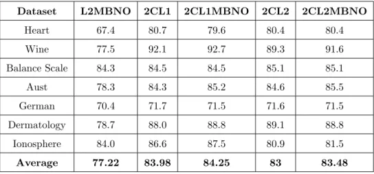
Table 4.3: Part 2 - KNN classification accuracy of 5 different algorithms: DL(L2,MBNO) de-noted by L2MBNO, DL2C(L1) denoted by 2CL1, DL2C(L1,MBNO) denoted by 2CL1MBNO, DL2C(L2,MBNO) denoted by 2CL2MBNO and DL2C(L2) denoted by 2CL2

Dataset L2MBNO 2CL1 2CL1MBNO 2CL2 2CL2MBNO

Heart 67.4 80.7 79.6 80.4 80.4 Wine 77.5 92.1 92.7 89.3 91.6 Balance Scale 84.3 84.5 84.5 85.1 85.1 Aust 78.3 84.3 85.2 84.6 85.5 German 70.4 71.7 71.5 71.6 71.5 Dermatology 78.7 88.0 88.8 89.1 88.8 Ionosphere 84.0 86.6 87.5 80.9 81.5 Average 77.22 83.98 84.25 83 83.48

(29)

19

Table 4.4: Part 1 - KNN classification accuracy of 5 different algorithms: Manhattan as Manh, Euclidean as Euc, DL(L1,GCG) denoted by L1GCG, DL(L1,MBNO) denoted by L1MBNO and DL(L2,GCG) denoted by L2GCG

Dataset Manh Euc L1GCG L1MBNO L2GCG

Breast Cancer Wisconsin 63.5 62.9 95.9 68.8 62.9

Habermans Survival 65.9 67.9 71.2 71.9 70.9 Diabetes 72.4 71.1 72.4 72.4 69.7 Statlog 63.6 62.9 63.3 63.3 62.2 Planning 61.5 64.3 68.7 63.2 65.9 Mammographic 73.5 73.7 75.9 78.1 77.0 ILDP 68.4 70.5 69.5 68.3 69.8 Congress 61.6 61.4 61.6 61.6 62.3 Average 66.3 66.83 72.31 68.45 67.58

Table 4.5: Part 2 - KNN classification accuracy of 5 different algorithms: DL(L2,MBNO) de-noted by L2MBNO, DL2C(L1) denoted by 2CL1, DL2C(L1,MBNO) denoted by 2CL1MBNO, DL2C(L2,MBNO) denoted by 2CL2MBNO and DL2C(L2) denoted by 2CL2

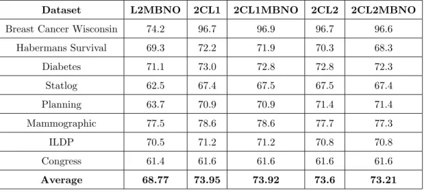
Dataset L2MBNO 2CL1 2CL1MBNO 2CL2 2CL2MBNO

Breast Cancer Wisconsin 74.2 96.7 96.9 96.7 96.6

Habermans Survival 69.3 72.2 71.9 70.3 68.3 Diabetes 71.1 73.0 72.8 72.8 72.3 Statlog 62.5 67.4 67.5 67.5 67.4 Planning 63.7 70.9 70.9 71.4 71.4 Mammographic 77.5 78.6 78.6 77.7 77.3 ILDP 70.5 71.2 71.2 70.8 70.8 Congress 61.4 61.6 61.6 61.6 61.6 Average 68.77 73.95 73.92 73.6 73.21

(30)

4.1. ACCURACY COMPARISON AMONG OUR DIFFERENT METHODS 20

4.1

Accuracy comparison among our different methods

In this section, we compare performance among our different methods based on a number of datasets. The methods that we include for comparision involvingL1 norm andL2 norm are DL(L1,MBNO), DL(L1,GCG), DL(L2,GCG) and DL(L2,MBNO) and then, we identify the best method which does not involve dist2C approach.

In this section, we also evaluate and compare our dist2C methods on 15 different datasets. We performed experiments with both the error correction methods for each dataset and what we found that GCG involving dist2C was poor in performance than other methods of dist2C. So, we have excluded it in the comparison and have only used dist2C involving MBNO (error correction) for the comparisons. Finally, we identify our best error correction method.

4.1.1

Comparison among different methods involving

L

1

norm

Table 4.2 and Table 4.4 compare different methods based on L1 norm named as: Manhattan, DL(L1,GCG) and DL(L1,MBNO). DL(L1,MBNO) and DL(L1,GCG) perform better than Manhat-tan in most of the datasets. If we compare the two methods with datasets listed in Table 4.2, DL(L1,GCG) wins the competition in almost all the datasets.

We have included some more experiment results in Table4.4with some harder datasets. Though there is some sort of competition between DL(L1,GCG) and DL(L1,MBNO) with datasets in Ta-ble 4.4, winner based on average performance is again DL(L1,GCG). Hence, we can say that DL(L1,GCG) is the best method based on L1 norm and performs consistently better and by good margin of 4.75% on dataset listed in Table4.2and 3.86% on harder datasets listed in Table4.4.

4.1.2

Comparison among different methods involving

L

2

norm

Here we compare and analyze different methods involving L2 norm. Table 4.2 and Table 4.3 show the performance of three methods named as: Euclidean, DL(L2,GCG) and DL(L2,MBNO). DL(L2,GCG) and DL(L2,MBNO) consistently perform better than Euclidean. DL(L2,MBNO) was better than DL(L2,GCG) on some datasets but DL(L2,GCG) wins the race by a margin of 3.4% on many datasets.

If we compare their performance on harder datasets available in Table 4.4 and Table 4.5, the result is quite different from above as DL(L2,MBNO) wins the race by small margin of 1.19%. Hence, we can say that these two methods are slightly different in performance. However on the basis of average performance, DL(L2,GCG) is the best method.

(31)

4.1. ACCURACY COMPARISON AMONG OUR DIFFERENT METHODS 21

4.1.3

Best method not involving dist2C approach

DL(L1,GCG) is the best method among methods involving L1 norm. The performance is quite similar between DL(L2,MBNO) and DL(L2,GCG). So, if we compare among these three methods, we can see that DL(L1,GCG) performs better than other two methods in almost all of the datasets. DL(L1,GCG) wins the race by large margin even with harder datasets. DL(L1,GCG) is better than DL(L2,GCG) by 3.5% on dataset in Table4.1. It is also better than DL(L1,MBNO) by margin of 3.54% on harder datsets. With all the comparisons above, we can finally say that DL(L1,GCG) is the best method among all the methods based onL1norm andL2norm without involving dist2C approach.

4.1.4

Comparison among different methods of Two-constant involving

L

1

norm

Table4.3presents results of different methods of dist2C based onL1norm. Though DL2C(L1,MBNO) is better than DL2C(L1) by small margin of 0.27%, there were some datsets like german and heart where DL2C(L1) performed better.

The case is quite different with harder dataset listed in Table4.5where DL2C(L1) lead by small margin of 0.03%. Hence, we can say that both the methods are almost equal in performance. On the basis of average performance, DL2C(L1,MBNO) is the best method.

4.1.5

Comparison among different methods on Two-constant involving

L

2

norm

DL2C(L2,MBNO) and DL2C(L2) performed better than Euclidean on most of the datasets. Though DL2C(L2,MBNO) is better than DL2C(L2) by 0.48%, we cannot draw a conclusion stating that DL2C(L2,MBNO) is always better.

There are many cases where DL2C(L2,MBNO) did not improve performance of the datasets like dermatology, heart, balance scale and german as shown in Table 4.3. If we see the results with harder datsets listed in Table4.5, DL2C(L2) wins the battle in most of the datasets by 0.39%. So, we cannot be sure for a certain method will perform better every time as the performance of both the methods are quite similar. However on the basis of average performance, DL2C(L2,MBNO) is the best method.

(32)

4.2. TOP TWO WINNERS (BEST) METHODS 22

4.1.6

Accuracy comparison between MBNO and GCG

In this part we compare between two error correction methods based on the results in different tables. If we takeL1norm orL2norm as starter function then GCG performed better than MBNO on the basis of average performances.

If we take dist2C approach, MBNO is better than GCG by significant margin.

4.2

Top two winners (best) methods

In this section we will identify two best methods among our methods. Almost all of our meth-ods enhanced the performance consistently by significant margin in comparison with Euclidean or Manhattan. They performed better with most of the datasets in Table4.1.

Two-constant approach was the most consistent which outplayed most of the other methods involving L1 norm or L2 norm as the starter function except DL(L1,GCG). It turned out that DL(L1,GCG) was almost equal in performance with methods based on dist2C approach.

After all the comparisons above, we elected two best methods from our methods. There were small margin (0.07%-1.61%) of performance differences among different methods involving dist2C and DL(L1,GCG). So, it was not easy to choose the top two best methods as any addition of dataset may change the top two winners.

However, on average performance of top 7 datasets in Table 4.1, DL(L1,GCG) is the first best method and DL2C(L1,MBNO) is the second best method.

4.3

Accuracy comparison between our two best methods and

some popular metric learning methods

This part deals with accuracy comparison between our two best methods and other popular metric learning methods: Large Margin Nearest Neighbor(LMNN) [Weinberger et al. 2005] and Information-Theoretic Metric Learning(ITML) [Davis et al. 2007]. In addition, we include non-metric learning method SVM [Crammer and Singer 2001] to compare with our existing methods.

Though most of our methods performed significantly better with most of the datasets, only few were competitive with the three popular methods. DL(L1,GCG) and DL2C(L1,MBNO) were the two best methods which consistently performed better with different datasets and we elected them to compare. For comparison of our two best methods with 3 popular methods, we are going to take

(33)

4.4. INSIGHTS ON ATTRIBUTE IMPORTANCE (WEIGHT) 23 7 data sets downloaded from UCI machine learning repository. Table4.1depicts summary of the 7 datasets.

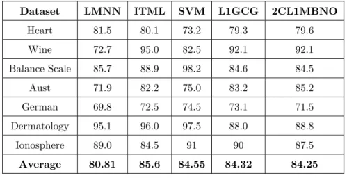
Table 4.6: Classification accuracy of 5 different algorithms: DL2C(L1,MBNO) denoted by 2CL1MBNO, DL(L1,GCG) denoted by L1GCG, Large Margin Nearest Neighbor (LMNN), Information-Theoretic Metric Learning (ITML) and Support Vector Machine (SVM)

Dataset LMNN ITML SVM L1GCG 2CL1MBNO

Heart 81.5 80.1 73.2 79.3 79.6 Wine 72.7 95.0 82.5 92.1 92.1 Balance Scale 85.7 88.9 98.2 84.6 84.5 Aust 71.9 82.2 75.0 83.2 85.2 German 69.8 72.5 74.5 73.1 71.5 Dermatology 95.1 96.0 97.5 88.0 88.8 Ionosphere 89.0 84.5 91 90 87.5 Average 80.81 85.6 84.55 84.32 84.25

Table 4.6 shows the performance of the two best methods with three popular methods for 7 different datasets. From Table 4.6, it is clear that the above three popular methods (LMNN, ITML,and SVM) clearly perform better with most of the datasets. On average DL(L1,GCG) and DL2C(L1,MBNO) performed better than LMNN (by margin of 3.44%-3.51%) but was slightly poor than ITML (by margin of 1.28%-1.35%) and SVM(by 0.23%-0.3%).

Though ITML and SVM win the competition by small margin, our methods performed better than ITML or SVM on some of the datasets. Our methods performed better than SVM with datasets like heart, wine and aust. Similarly, our methods performed better than ITML with datasets like aust, german and ionosphere. So, our methods perform better on some datasets where other methods fail to perform good.

4.4

Insights on Attribute Importance (Weight)

In this section, we talk about insights on importance of attributes. As we have discussed earlier that the weight of an attribute can be positive, negative or zero. Here, we rank the attributes based on their weight change. We performed experiments where we computed percentage of each weight based on total weight of the attributes. Then we computed accuracy change and percent change

(34)

4.4. INSIGHTS ON ATTRIBUTE IMPORTANCE (WEIGHT) 24 for corresponding attributes of two different methods. The comparison was done between our best methods and the corresponding L norm.

Table 4.7: Top 2 positive big change attributes and top 2 negative big change attributes

Dataset Positive Big Change Negative Big Change

Balance Scale A3, A1 A2, A4

Heart A9, A12 A6, A10

Wine A11, A12 A6, A9

Congress A8, A11 A5, A3

Breast Cancer Wisconsin A7, A3 A1, A10

Aust A8, A9 A12, A1

German A19, A21 A15, A18

Planning A10, A4 A11, A6

Statlog A1, A5 A6, A12

Diabetes A1, A2 A3, A5

Dermatology A31, A15 A30, A23

Ionosphere A1, A3 A13, A19

The available attributes name for some datasets are given as follows:

Balance Scale: A3 (Right Weight), A1 (Left Weight), A2 (Left Distance), and A0 ( Right Distance) Heart: A9 (Exercise induced angina), A12 (Number of major vessels (0-3) colored by flourosopy), A6 (fasting blood sugar>120 mg/dl) and A10 (ST depression induced by exercise relative to rest) Wine: A11 (Hue), A12 (OD280/OD315 of diluted wines), A6 (Total phenols and A9:

Proanthocyanins)

Congress: A8 (aid-to-nicaraguan-contras), A11 ( synfuels-corporation-cutback), A5 (el-salvador-aid) and A3 (adoption-of-the-budget-resolution)

Breast Cancer Wisconsin: A7 (Bare Nuclei), A3 (Uniformity of Cell Size), A1 (Sample code number) and A10 (Mitoses)

We rank the attributes into two categories: positive big change attributes and negative big change attributes . Positive big change attributes are those attributes which have big positive weight change and add to the total distance. Negative big change attributes are those attributes which have big negative weight change and deduct from the total distance. They bring tuples closer than before. In

(35)

4.4. INSIGHTS ON ATTRIBUTE IMPORTANCE (WEIGHT) 25 this part, we find the top 2 positive big change attributes and top 2 negative big change attributes for some datasets in Table4.1.

Table 4.7 presents top two positive big change attributes and top two negative big change at-tributes of different datasets available in Table4.1.

Table 4.8: Impact of different values ofγon GCG

Dataset Method γ (0.2) γ(0.8) γ(2.0) γ(5.0) Wine L2GCG 76.4045 75.8427 66.2921 61.236 Wine L1GCG 92.1348 92.1348 91.0112 90.4494 Wine 2CL1GCG 92.1348 92.1348 91.0112 90.4494 Wine 2CL2GCG 76.4045 75.8427 66.8539 61.7978 Planning L2GCG 64.8352 65.3846 65.9341 65.9341 Planning L1GCG 64.8352 65.3846 67.5824 67.5824 Planning 2CL1GCG 64.8352 65.3846 67.033 68.1319 Planning 2CL2GCG 64.8352 65.3846 65.9341 65.9341 Heart L2GCG 83.3333 83.3333 82.2222 81.8519 Heart L1GCG 82.2222 82.5926 82.2222 82.2222 Heart 2CL1GCG 82.2222 82.5926 82.2222 82.2222 Heart 2CL2GCG 83.3333 83.3333 82.2222 81.8519 Habermans survival L2GCG 67.6471 67.6471 67.6471 67.9739 Habermans survival L1GCG 68.6275 68.6275 68.6275 68.6275 Habermans survival 2CL1GCG 68.6275 68.6275 68.6275 68.6275 Habermans survival 2CL2GCG 67.6471 67.6471 67.9739 67.9739 Breast cancer wisconsin L2GCG 94.32 94.32 94.32 94.32 Breast cancer wisconsin L1GCG 93.5622 94.7067 95.7082 95.9943 Breast cancer wisconsin 2CL1GCG 93.5622 94.7067 95.7082 95.9943 Breast cancer wisconsin 2CL2GCG 94.32 94.32 94.32 94.32 Note: DL(L1,GCG) denoted by L1GCG, DL(L2,GCG) denoted by L2GCG, DL2C(L1,GCG) denoted by 2CL1GCG and DL2C(L2,GCG) denoted by 2CL2GCG

(36)

4.5. IMPACT OF PARAMETERS ON OUR METHODS 26

Table 4.9: Impact of different values ofν on MBNO

Dataset Method ν(5) ν(10) ν(15) Heart L2MBNO 66.2963 82.5926 81.4815 Heart L1MBNO 71.4815 82.2222 82.2222 Heart 2CL1MBNO 82.2222 82.2222 82.2222 Heart 2CL2MBNO 82.5926 82.2222 81.4815 Wine L2MBNO 70.2247 94.9438 94.9438 Wine L1MBNO 71.9101 96.0674 96.0674 Wine 2CL1MBNO 96.0674 96.0674 96.0674 Wine 2CL2MBNO 94.9438 94.9438 94.9438 Planning L2MBNO 63.7363 71.4286 71.4286 Planning L1MBNO 60.989 71.4286 71.4286 Planning 2CL1MBNO 71.4286 71.4286 71.4286 Planning 2CL2MBNO 71.4286 71.4286 71.4286 Habermans survival L2MBNO 66.6667 68.6275 68.6275 Habermans survival L1MBNO 66.9935 66.3399 66.6667 Habermans survival 2CL1MBNO 66.3399 66.3399 66.9935 Habermans survival 2CL2MBNO 67.9739 68.6275 68.3007 Breast cancer wisconsin L2MBNO 53.7911 95.9943 95.9943 Breast cancer wisconsin L1MBNO 64.8069 95.422 95.422 Breast cancer wisconsin 2CL1MBNO 95.422 95.422 95.422 Breast cancer wisconsin 2CL2MBNO 96.1373 95.9943 95.9943 Note: DL(L1,MBNO) denoted by L1MBNO, DL(L2,MBNO) denoted by L2MBNO,

DL2C(L1,MBNO) denoted by 2CL1MBNO and DL2C(L2,MBNO) denoted by 2CL2MBNO

4.5

Impact of parameters on our methods

In this section, we describe the impact of our various parameters on our methods. We have chosen γand ν to discuss in this section. Since these parameters depend on the user, we need to know its impact on the performance. We have chosen 4 different values ofγand 3 different values ofν. We tested the result on 5 different datasets taking k as 5 andd1for same class distance as 5 andd2 for different class distance as 25.

(37)

4.6. CHECKING THE CONSISTENCY OF OUR METHODS 27 After analyzing Table4.8, we can say that GCG performs better when the value of γ is 0.2 or 0.8. With the increasing value ofγ, there is some sudden drop in performance for some methods.

After analyzing Table4.9, we can say that MBNO performs better with larger value ofν. ν=5 did not give better result in comparison with other larger values. After all the discussions, we can say that 2∗kis the optimum value forν as a parameter of MBNO.

4.6

Checking the consistency of our methods

In this section, we performed experiments on different datasets using 5 folds cross validation so that we can evaluate the consistency of our methods. Table4.10and Table4.11show the result of our different methods. In the tables, the result is in the form of num1±num2 where num1 is the mean classification accuracy in percentage and num2 is the deviation of accuracy in percentage. num1±num2 shows that the result varies fromnum1−num2 tonum1 +num2. From the tables, we can say that our methods were quite consistent. However, DL(L1,GCG) was the most consistent among our different methods.

Table 4.10: Part 1 - KNN classification accuracy of 6 different algorithms: Manhattan as Manh, Euclidean as Euc, DL(L1,GCG) denoted by L1GCG, DL(L1,MBNO) denoted by L1MBNO, DL(L2,MBNO) denoted by L2MBNO and DL(L2,GCG) denoted by L2GCG

Dataset Manh Euc L1GCG L1MBNO L2GCG L2MBNO

Wine 73±5 70±8 92±5 75±6 76±10 76±9 Aust 71±4 71±4 79±4 74±4 74±4 79±3 Heart 70±4 67±5 77±4 71±3 79±8 67±7 Balance scale 81±4 82±2 84±2 86±4 84±2 86±3 German 67±2 68±3 72±2 70±4 70±3 69±1 Planning 65±7 63±8 64±4 65±5 64±7 63±7 Diabetes 72±2 70±3 72±1 72±2 72±3 70±5

(38)

4.6. CHECKING THE CONSISTENCY OF OUR METHODS 28

Table 4.11: Part 2 - KNN classification accuracy of 6 different algorithms: DL2C(L1) denoted by 2CL1, DL2C(L1,MBNO) denoted by 2CL1MBNO, DL2C(L1,GCG) denoted by 2CL1GCG, DL2C(L2,GCG) denoted by 2CL2GCG, DL2C(L2,MBNO) denoted by 2CL2MBNO and DL2C(L2) denoted by 2CL2

Dataset 2CL1 2CL1GCG 2CL1MBNO 2CL2 2CL2GCG 2CL2MBNO

Wine 92±2 92±2 92±3 94±3 76±7 94±3 Aust 83±2 79±6 84±2 85±3 74±4 84±2 Heart 81±10 77±7 81±7 82±8 79±5 83±7 Balance scale 84±2 84±2 84±2 85±2 84±1 85±2 German 71±1 72±2 71±1 70±1 70±3 70±1 Planning 70±3 64±5 70±3 71±2 64±10 71±2 Diabetes 73±2 72±1 73±2 74±3 72±5 73±4

(39)

5

Related Work

Distance metric learning has been an active area of research and it is not practical to include and discuss all the related works. So, in this chapter we briefly review most related representatives on this topic.

The recent proposed metric learning method [Weinberger et al. 2005] LMNN targets to bring same class neighbors of KNN closer while different class neighbors are separated by large margin. It incorporates Mahalanobis distance metric by semidefinite programming to meet the requirements for k-nearest neighbor classification (KNN).

LMNN used cost function to penalize large distances and small distances between class instances and the cost function as an instance of semidefinite programming can be given as:

MinimizeP

ijηij(x~i−x~j)TM(x~i−x~j) +cPijηij(1−yil)εijl subject to:

• (x~i−x~l)TM(x~i−x~l)−(x~i−x~j)TM(x~i−x~j)≥1-εijl

• εijl≥0

• M≥0.

where (x~i, ~yi) denote a training set with inputs x~i∈Rd and class labelsyi. ηij to indicate whether inputx~jis a target neighbor of inputx~i,M=LTL,L:Rd→Rd, c is a positive constant (typically set by cross validation) and slack variables (hinge loss)εijlfor all pairs of differently labeled inputs.

The first term in the above expression penalizes large distance between target neighbors and each input, and the second term penalizes small distances between each input and all other inputs that have different class labels.

(40)

30 Our idea is quite similar in spirit but different in formulas and technicality than that of LMNN because we penalize only the small distance from test input with k-nearest neighbors which has dif-ferent class labels than that of test input. We penalize small distances only when their presence leads to KNN classification error. We have employed error correction method MBNO which performs the above operation. We have two more approaches GCG and the Two-constant which is quite different from LMNN. One more difference between our approach and LMNN is that we used Euclidean and Manhattan for distance metric learning whereas LMNN used Mahalanobis distance metric.

One of the recent work, [Davis et al. 2007] presented an approach to learn a Mahalanobis dis-tance function by information-theoretic approach. It formulates the metric learning problem by minimizing the differential relative entropy between two multivariate Gaussians under constraints. It uses techniques of minimizing the LogDet divergence subject to linear constraints. It considers a relationship constraining the similarity and dissimilarity between pair of points. It considers two points are similar if the Mahalanobis distance between them is smaller than a threshold value (upper bound). Similarly, two points belong to different class labels if distance between them is larger than a threshold value (lower bound). The main framework of learning the distance function is:

Given pairs of similar points denoted by S and pairs of dissimilar points denoted by D, the metric problem is:

minA KL(p(x;A0)||p(x;A)) subject to

• dA(xi, xj)≤u(i, j)∈S,

• dA(xi, xj)≥l (i, j)∈D,

where Mahalanobis distance is defined as : dA(xi, xj) = (xi−xj)TA(xi−xj), (x1, ..., xn) are real numbers and A is a positive definite matrix.

Distance between two Mahalanobis distance functions parametrized by A0 and A by relative entropy between multivariate Gaussians:

KL(p(x;A0)||p(x;A))= R p(x;A0)log p(x;A0) p(x;A)dx wherep(x;A) =_Z1exp(−1

2dA(x, µ)) is the multivariate Gaussian.

Our work is inspired by similar spirit but our error correction part is more intuitive than ITML method. We perform error correction (GCG) such that minimum distance among different class la-bels should be larger than maximum distance among same class lala-bels. Our method learns weighted Euclidean or weighted Manhattan distance functions whereas ITML learns Mahalanobis distance

(41)

31 functions.

In [Chopra et al. 2005], the authors presented a framework for training a similarity metric by energy-based model (EBM). The authors formulate the loss function such that it penalizes large distances among examples with the same label, and small distance among different class labels pairs. ”The method is applied to a face verification task. The learning process minimizes a discriminative loss function that drives the similarity metric to be small for pairs of faces from the same person, and large for pairs from different persons. The mapping from raw to the target space is a convolutional network whose architecture is designed for robustness to geometric distortions. The system is tested on the Purdue/AR face database which has a very high degree of variability in the pose, lighting, expression, position, and artificial occlusions such as dark glasses and obscuring scarves.” In our work, we learn the metric with similar essence but with different approach and formulas where we penalize the large distance among different class labels as in GCG.

(42)

6

Conclusion

This chapter summarizes our methods, experimental results and findings. It also discuss future works for this thesis.

6.1

Summary

Distance metric learning is one of the widely used element of machine learning community and it’s impact is effective and notable. In this thesis, we learn weighted distance function by applying linear regression on idealized distance functions. Identifying the importance of attributes and assigning weight to them uncovers optimal relationship between distance and the attributes.

This thesis introduced a novel method of weighted distance function learning using idealized distance functions. The metric is trained with the goal that same class neighbors should be closer (small distance) while different class neighbors separated by large distance. Chapter 3 presented 3 approach of ideal distance computation named as: Move Bad Neighbors Out (MNBO), 2)Global Class Gap (GCG) and 3) Two-constant approach and two algorithms to perform our weighted distance learning.

In chapter4, we gave experimental results on 15 datasets to evaluate our different methods. We used KNN to measure the effectiveness of our approach. Our experiments showed that our metric learning methods performed better than LMNN. Though ITML and SVM were better than our methods in performance, our methods performed better at some datasets. Finally we gave some insights on the attributes importance of different datasets.

It is interesting to note that by applying linear regression to the idealized distance, we can get better result. Linear regression on idealized distance performed better than some of the popular methods. We can even say that KNN classification accuracy can improve if provided better distance

(43)

6.2. FUTURE WORK 33 metric. Similarly, any distance based classification or regression can improve if provided better distance metric.

6.2

Future Work

In this work, we identified the potential of improving our weighted distance metric learning. Since we used linear regression to learn our distance function, there is prospective for better distance metric by employing better regression analysis. In [Dong and Taslimitehrani 2015], it has been shown how a contrast pattern aided regression method (CPXR) can outperform state-of-the-art regression methods by big margins. So, CPXR as a regression method can be used to learn distance metric giving more competitive result.

(44)

References

Chopra, S.,Hadsell, R.,and LeCun, Y.2005. Learning a similarity metric discriminatively,

with application to face verification. 2005 IEEE Computer Society Conference on Computer

Vision and Pattern Recognition (CVPR 2005), 20-26 June 2005, San Diego, CA, USA, 539–546.

Cover, T. M. and Hart, P. E. 1967. Nearest neighbor pattern classification. IEEE Trans.

Information Theory 13,1, 21–27.

Crammer, K. and Singer, Y. 2001. On the algorithmic implementation of multiclass kernel-based vector machines. Journal of machine learning research 2,Dec, 265–292.

Davis, J. V.,Kulis, B., Jain, P.,Sra, S., and Dhillon, I. S.2007. Information-theoretic

metric learning. Machine Learning, Proceedings of the Twenty-Fourth International Conference

(ICML 2007), Corvallis, Oregon, USA, June 20-24, 2007, 209–216.

Dong, G. and Taslimitehrani, V. 2015. Pattern-aided regression modeling and prediction

model analysis. IEEE Trans. Knowl. Data Eng. 27,9, 2452–2465.

Goldberger, J.,Roweis, S. T.,Hinton, G. E.,and Salakhutdinov, R.2004. Neighbour-hood components analysis. Advances in Neural Information Processing Systems 17 [Neural In-formation Processing Systems, NIPS 2004, December 13-18, 2004, Vancouver, British Columbia,

Canada], 513–520.

Hastie, T. and Tibshirani, R. 1995. Discriminant adaptive nearest neighbor classification.

Proceedings of the First International Conference on Knowledge Discovery and Data Mining

(KDD-95), Montreal, Canada, August 20-21, 1995, 142–149.

Luan, C. and Dong, G. 2017. Experimental identification of hard data sets for classification

and feature selection methods with insights on method selection. CoRR abs/1703.08283.

(45)

6.2. FUTURE WORK 35

Nguyen, N. and Guo, Y.2008. Metric learning: A support vector approach.Machine Learning

and Knowledge Discovery in Databases, European Conference, ECML/PKDD 2008, Antwerp,

Belgium, September 15-19, 2008, Proceedings, Part II, 125–136.

Schultz, M. and Joachims, T. 2003. Learning a distance metric from relative comparisons.

Advances in Neural Information Processing Systems 16 [Neural Information Processing Systems,

NIPS 2003, December 8-13, 2003, Vancouver and Whistler, British Columbia, Canada], 41–48.

Shalev-Shwartz, S.,Singer, Y.,and Ng, A. Y.2004. Online and batch learning of

pseudo-metrics. Machine Learning, Proceedings of the Twenty-first International Conference (ICML

2004), Banff, Alberta, Canada, July 4-8, 2004.

Tsang, I. W., Kwok, J. T., and Bay, C. W.2003. Distance metric learning with kernels.

Proceedings of the International Conference on Artificial Neural Networks, 126–129.

Weinberger, K. Q.,Blitzer, J.,and Saul, L. K. 2005. Distance metric learning for large margin nearest neighbor classification. Advances in Neural Information Processing Systems 18 [Neural Information Processing Systems, NIPS 2005, December 5-8, 2005, Vancouver, British

Columbia, Canada], 1473–1480.

Xing, E. P.,Ng, A. Y.,Jordan, M. I., and Russell, S. J.2002. Distance metric learning

with application to clustering with side-information. Advances in Neural Information Processing Systems 15 [Neural Information Processing Systems, NIPS 2002, December 9-14, 2002,

CORE Scholar CORE Scholar

Browse all Theses and Dissertations

Theses and Dissertations

works at: https://corescholar.libraries.wright.edu/etd_all

Computer Engineering Commons, and the

Computer Sciences Commons

https://corescholar.libraries.wright.edu/etd_all/1739