Discovering Petri Nets From Event Logs
W.M.P. van der Aalst and B.F. van Dongen Department of Mathematics and Computer Science, Technische Universiteit Eindhoven, The Netherlands.
{W.M.P.v.d.Aalst,B.F.v.Dongen}@tue.nl
Abstract. As information systems are becoming more and more inter-twined with the operational processes they support, multitudes of events are recorded by todays information systems. The goal ofprocess mining
is to use such event data to extract process related information, e.g., to automatically discover a process model by observing events recorded by some system or to check the conformance of a given model by com-paring it with reality. In this article, we focus onprocess discovery, i.e., extracting a process model from an event log. We focus on Petri nets as a representation language, because of the concurrent and unstructured na-ture of real-life processes. The goal is to introduce several approaches to discover Petri nets from event data (notably theα-algorithm, state-based regions, and language-based regions). Moreover, important requirements for process discovery are discussed. For example, process mining is only meaningful if one can deal with incompleteness (only a fraction of all possible behavior is observed) and noise (one would like to abstract from infrequent random behavior). These requirements reveal significant challenges for future research in this domain.
Keywords: Process mining, Process discovery, Petri nets, Theory of regions
1
Introduction
Process mining provides a new means to improve processes in a variety of appli-cation domains [2, 41]. There are two main drivers for this new technology. On the one hand, more and more events are being recorded thus providing detailed information about the history of processes. Despite the omnipresence of event data, most organizations diagnose problems based on fiction rather than facts. On the other hand, vendors of Business Process Management (BPM) and Busi-ness Intelligence (BI) software have been promising miracles. Although BPM and BI technologies received lots of attention, they did not live up to the expectations raised by academics, consultants, and software vendors.
Process mining is an emerging discipline providing comprehensive sets of tools to provide fact-based insights and to support process improvements [2, 7]. This new discipline builds on process model-driven approaches and data mining. However, process mining is much more than an amalgamation of existing ap-proaches. For example, existing data mining techniques are too data-centric to
provide a comprehensive understanding of the end-to-end processes in an organi-zation. BI tools focus on simple dashboards and reporting rather than clear-cut business process insights. BPM suites heavily rely on experts modeling ideal-ized to-be processes and do not help the stakeholders to understand the as-is processes.
Over the last decadeevent datahas become readily available and process min-ing techniques have matured. Moreover, process minmin-ing algorithms have been implemented in various academic and commercial systems. Examples of com-mercial systems that support process mining are: ARIS Process Performance Manager by Software AG, Disco by Fluxicon, Enterprise Visualization Suite by Businesscape,Interstage BPME by Fujitsu,Process Discovery Focus by Ion-tas, Reflect|one by Pallas Athena, andReflect by Futura Process Intelligence. Today, there is an active group of researchers working on process mining and it has become one of the “hot topics” in BPM research. Moreover, there is a huge interest from industry in process mining. This is illustrated by the recently released Process Mining Manifesto [41]. The manifesto is supported by 53 or-ganizations and 77 process mining experts contributed to it. The manifesto has been translated into a dozen languages (http://www.win.tue.nl/ieeetfpm/). The active contributions from end-users, tool vendors, consultants, analysts, and re-searchers illustrate the growing relevance of process mining as a bridge between data mining and business process modeling. Moreover, more and more software vendors started adding process mining functionality to their tools. The authors have been involved in the development of the open-source process mining tool ProM right from the start [11, 56, 57]. ProM is widely used all over the globe and provides an easy starting point for practitioners, students, and academics.
Whereas it is easy to discover sequential processes, it is very challenging to discover concurrent processes, especially in the context of noisy and incomplete event logs. Given the concurrent nature of most real-life processes, Petri nets are an obvious candidate to represent discovered processes. Moreover, most real-life processes are not nicely block-structured, therefore, the graph based nature of Petri nets is more suitable than notations that enforce more structure.
The article is based on a lecture given at the Advanced Course on Petri nets in Rostock, Germany (September 2010). The practical relevance of process discovery and the suitability of Petri net as a basic representation for concurrent processes motivated us to write this tutorial.
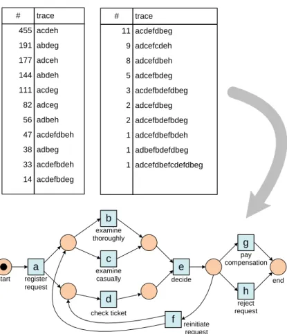
Figure 1 illustrates the concept of process discovery using a small example. The figure shows an abstraction of an event log. There are 1391 cases, i.e., process instances. Each case is described as a sequence of activities, i.e., a trace. In this particular log there are 21 different traces. For example, traceha, c, d, e, hi
occurs 455 times, i.e., there are 455 cases for which this sequence of activities was executed. The challenge is to discover a Petri net given such an event log. A discovery algorithm such as the α-algorithm [9] is able to discover the Petri net shown in Figure 1.
Process discovery is a challenging problem because one cannot assume that all possible sequences are indeed present. Consider for example the event log
a start register request b examine thoroughly c examine casually d check ticket decide pay compensation reject request reinitiate request e g h f end acdeh abdeg adceh abdeh acdeg adceg adbeh acdefdbeh adbeg acdefbdeh acdefbdeg 455 191 177 144 111 82 56 47 38 33 14 # trace acdefdbeg adcefcdeh adcefdbeh adcefbdeg acdefbdefdbeg adcefdbeg adcefbdefbdeg adcefdbefbdeh adbefbdefdbeg adcefdbefcdefdbeg 11 9 8 5 3 2 2 1 1 1 # trace
Fig. 1.A Petri net discovered from an event log containing 1391 cases.
shown in Figure 1. If we randomly take 500 cases from the set of 1391 cases, we would like to discover “more or less” the same model. Note that there are several traces that appear only once in the log. Many of these will disappear when considering a log with only 500 cases. Also note that the process model discovered by theα-algorithm allows for more traces than the ones depicted in Figure 1, e.g.,ha, d, c, e, f, d, b, e, f, c, d, e, hiis possible according to the process model but does not occur in the event log. This illustrates that event logs tend to befar from complete, i.e., only a small subset of all possible behavior can be observed because the number of variations is larger than the number of instances observed.
The process model in Figure 1 is rather simple. Real-life processes will consist of dozens or even hundreds of different activities. Moreover, some behaviors will be very infrequent compared to others. Such rare behaviors can be seen as
noise(e.g., exceptions). Typically, it is undesirable and also unfeasible to capture frequent and infrequent behavior in a single diagram.
Process discovery techniques need to be able to deal with noise and incom-pleteness. This makes process mining very different from synthesis. Classical synthesis techniques aim at creating a model that captures the given behavior precisely. For example, classical language-based region techniques [14, 17, 19, 28, 42, 43, 45] distill a Petri net from a (possibly infinite) language, such that the behavior of the Petri net is only minimally more than the given language. In classical state-based region theory [13, 15, 23, 24, 26, 27, 35] on the other hand, a transition system is used to synthesize a Petri net of which the behavior is bisimilar with the given transition system. Intuitively two models are bisimilar if they can match each other’s moves, i.e., they cannot be distinguished from one another by an observer [36]. In terms of mining this implies that the na¨ıvely synthesized Petri net cannot generalize beyond the example traces seen.
Process discovery techniques need to balance four criteria:fitness (the dis-covered model should allow for the behavior seen in the event log),precision(the discovered model should not allow for behavior completely unrelated to what was seen in the event log),generalization(the discovered model should generalize the example behavior seen in the event log), and simplicity (the discovered model should be as simple as possible). This makes process discovery a challenging and highly relevant topic.
The remainder of this article is organized as follows. Section 2 introduces the process mining spectrum showing that process discovery is an essential ingre-dient for process analysis based on facts rather than fiction. Section 3 presents preliminaries and formalizes the process discovery task. Theα-algorithm is pre-sented in Section 4. Section 5 discusses the main challenges related to process mining. In Section 6, we compare process discovery with region theory in more detail. This section shows that classical approaches cannot deal with partic-ular requirements essential for process mining. Then, in sections 7 and 8, we show how region theory can be adapted to deal with these requirements. Both state-based regions and language-based regions are considered. All approaches described in this article are supported byProM, the leading open-source process mining framework. ProM is described in Section 9. Section 10 ends this article with some conclusions and challenges that remain.
2
Process Mining
Process mining is an important tool for modern organizations that need to man-age non-trivial operational processes. On the one hand, there is an incredible growth of event data [44]. On the other hand, processes and information need to be aligned perfectly in order to meet requirements related to compliance, effi-ciency, and customer service.Process mining is much broader than just control-flow discovery, i.e., discovering a Petri net from a multi-set of traces. Therefore, we start by providing an overview of the process mining spectrum.
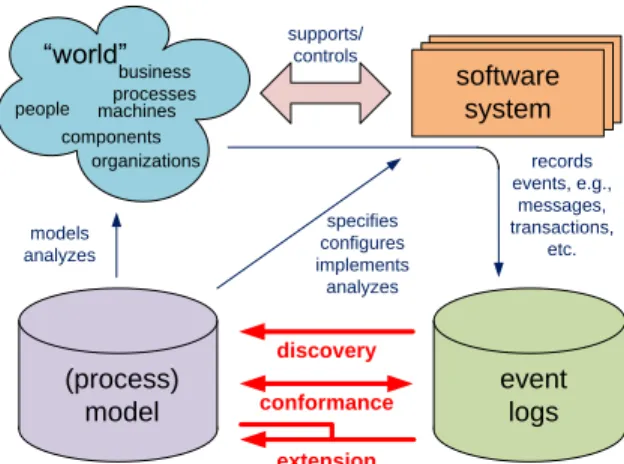
software system (process) model event logs models analyzes discovery records events, e.g., messages, transactions, etc. specifies configures implements analyzes supports/ controls extension conformance “world” people machines organizations components business processes
Fig. 2.Positioning of the three main types of process mining:discovery,conformance,
andenhancement.
Event logs can be used to conduct three types of process mining as shown in Figure 2 [2, 7].
The first type of process mining is discovery. A discovery technique takes an event log and produces a model without using any a-priori information. An example is theα-algorithm [9] that will be described in Section 4. This algorithm takes an event log and produces a Petri net explaining the behavior recorded in the log. For example, given sufficient example executions of the process shown in Figure 1, the α-algorithm is able to automatically construct the Petri net without using any additional knowledge. If the event log contains information about resources, one can also discover resource-related models, e.g., a social network showing how people work together in an organization.
The second type of process mining isconformance. Here, an existing process model is compared with an event log of the same process. Conformance checking can be used to check if reality, as recorded in the log, conforms to the model and vice versa. For instance, there may be a process model indicating that purchase orders of more than one million Euro require two checks. Analysis of the event log will show whether this rule is followed or not. Another example is the checking of the so-called “four-eyes” principle stating that particular activities should not be executed by one and the same person. By scanning the event log using a model specifying these requirements, one can discover potential cases of fraud. Hence, conformance checking may be used to detect, locate and explain deviations, and to measure the severity of these deviations. An example is the conformance checking algorithm described in [51]. Given the model shown in Figure 1 and a corresponding event log, this algorithm can quantify and diagnose deviations. In [4] another approach based on creatingalignmentsis presented. An alignment isoptimal if it relates the trace in the log to a most similar path in the model.
After creating optimal alignments, all behavior in the log can be related to the model.
The third type of process mining isenhancement. Here, the idea is to extend or improve an existing process model using information about the actual pro-cess recorded in some event log. Whereas conformance checking measures the alignment between model and reality, this third type of process mining aims at changing or extending the a-priori model. One type of enhancement is repair, i.e., modifying the model to better reflect reality. For example, if two activities are modeled sequentially but in reality can happen in any order, then the model may be corrected to reflect this. Another type of enhancement isextension, i.e., adding a new perspective to the process model by cross-correlating it with the log. An example is the extension of a process model with performance data. For instance, Figure 1 can be extended with information about resources, decision rules, quality metrics, etc.
The Petri net in Figure 1 only shows the control-flow. However, when extend-ing process models, additional perspectives need to be added. Moreover, discov-ery and conformance techniques are not limited to control-flow. For example, one can discover a social network and check the validity of some organizational model using an event log. Hence, orthogonal to the three types of mining (dis-covery, conformance, and enhancement), different perspectives can be identified. Theorganizational perspectivefocuses on information about resources hidden in the log, i.e., which actors (e.g., people, systems, roles, and departments) are in-volved and how are they related. The goal is to either structure the organization by classifying people in terms of roles and organizational units or to show the social network. Thetime perspectiveis concerned with the timing and frequency of events. When events bear timestamps it is possible to discover bottlenecks, measure service levels, monitor the utilization of resources, and predict the re-maining processing time of running cases.
3
Process Discovery: Preliminaries and Purpose
In this section, we describe the goal of process discovery. In order to do this, we present a particular format for logging events and a particular process modeling language (i.e., Petri nets). Based on this we sketch various process discovery approaches.
3.1 Event Logs
The goal of process mining is to extract knowledge about a particular (oper-ational) process from event logs, i.e., process mining describes a family of a-posteriorianalysis techniques exploiting the information recorded in audit trails, transaction logs, databases, etc. Typically, these approaches assume that it is possible to sequentially record events such that each event refers to an activ-ity (i.e., a well-defined step in the process) and is related to a particular case (i.e., a process instance). Furthermore, some mining techniques use additional
information such as the performer ororiginator of the event (i.e., the person / resource executing or initiating the activity), thetimestampof the event, ordata elements recorded with the event (e.g., the size of an order).
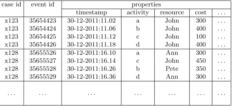
To clarify the notion of an event log consider Table 1 which shows a fragment of some event log. Only two traces are shown, both containing four events. Each event has a unique id and several properties. For example event 35654423 belongs to casex123 and is an instance of activityathat occurred on December 30th at 11.02, was executed by John, and cost 300 euros. The second trace (casex128) starts with event 35655526 and also refers to an instance of activity a. The
Table 1.A fragment of some event log.
case id event id properties
timestamp activity resource cost . . .
x123 35654423 30-12-2011:11.02 a John 300 . . . x123 35654424 30-12-2011:11.06 b John 400 . . . x123 35654425 30-12-2011:11.12 c John 100 . . . x123 35654426 30-12-2011:11.18 d John 400 . . . x128 35655526 30-12-2011:16.10 a Ann 300 . . . x128 35655527 30-12-2011:16.14 c John 450 . . . x128 35655528 30-12-2011:16.26 b Pete 350 . . . x128 35655529 30-12-2011:16.36 d Ann 300 . . . . . . .
information depicted in Table 1 is the typical event data that can be extracted from today’s systems.
Systems store events in very different ways. Process-aware information sys-tems (e.g., workflow management syssys-tems) provide dedicated audit trails. In other systems, this information is typically scattered over several tables. For example, in a hospital events related to a particular patient may be stored in different tables and even different systems. For many applications of process mining, one needs to extract event data from different sources, merge these data, and convert the result into a suitable format. We advocate the use of the so-called XES (eXtensible Event Stream) format that can be read directly by ProM ( [5, 57]). XES is the successor of MXML. Based on many practical expe-riences with MXML, the XES format has been made less restrictive and truly extendible. In September 2010, the format was adopted by the IEEE Task Force on Process Mining. The format is supported by tools such as ProM (as of ver-sion 6), Nitro, XESame, and OpenXES. See www.xes-standard.org for detailed information about the standard. XES is able to store the information shown in Table 1. Most of this information is optional, i.e., if it is there, it can be used for process mining, but it is not necessary for control-flow discovery.
In this article, we focus on control-flow discovery. Therefore, we only consider the activity column in Table 1. This means that an event is linked to a case (process instance) and an activity, and no further attributes are needed. Events are ordered (per case), but do not need to have explicit timestamps. This allows us to use the following simplified definition of an event log.
Definition 1 (Event, Trace, Event log).LetAbe a set of activities.σ∈A∗ is a trace, i.e., a sequence of events.L∈IB(A∗)is an event log, i.e., a multi-set of traces.
The first four events in Table 1 form a traceha, b, c, di. This trace represents the path followed by casex123. The second case (x128) can be represented by the traceha, c, b, di. Note that there may be multiple cases that have the same trace. Therefore, an event log is defined as amulti-set of traces.
A multi-set (also referred to as bag) is like a set where each element may occur multiple times. For example, [horse,cow5,duck2] is the multi-set with eight elements: one horse, five cows and two ducks. IB(X) is the set of multi-sets (bags) overX. We assume the usual operators on multi-sets, e.g.,X∪Y is the union of X and Y,X\Y is the difference betweenX andY,x∈X tests ifxappears inX, andX ≤Y evaluates to true ifX is contained inY. For example, [horse,cow2]∪ [horse2,duck2] = [horse3,cow2,duck2], [horse3,cow4]\[cow2] = [horse3,cow2], [horse,cow2] ≤ [horse2
,cow3], and [horse3
,cow1] 6≤ [horse2
,cow2]. Note that sets can be considered as bags having only one instance of every element. Hence, we can mix sets and bags, e.g.,{horse,cow} ∪[horse2,cow3] = [horse3
,cow4]. For practical applications of process mining it is essential to differentiate be-tween traces that are infrequent or even unique (multiplicity of 1) and traces that are frequent. Therefore, an event log is a multi-set of traces rather than an ordinary set. However, in this article we focus on the foundations of process discovery thereby often abstracting from noise and frequencies. See [2] for tech-niques that take frequencies into account. This book also describes various case studies showing the importance of multiplicities.
In the remainder, we will use the following example log: L1 = [ha, b, c, di5, ha, c, b, di8,ha, e, di9].L
1contains information about 22 cases; five cases following trace ha, b, c, di, eight cases following trace ha, c, b, di, and nine cases following trace ha, e, di. Note that such a simple representation can be extracted from sources such as Table 1, MXML, XES, or any other format that links events to cases and activities.
3.2 Petri Nets
The goal of process discovery is to distil a process model from some event log. Here we use Petri nets [50] to represent such models. In fact, we extract a subclass of Petri nets known as workflow nets (WF-nets) [1].
Definition 2. An Petri netis a tuple (P, T, F)where: 1. P is a finite set of places,
2. T is a finite set of transitions such thatP∩T =∅, and
3. F⊆(P×T)∪(T×P)is a set of directed arcs, called the flow relation. An example Petri net is shown in Figure 3. This Petri net has six places represented by circles and four transitions represented by squares. Places may contain tokens. For example, in Figure 3 both p1 and p6 contain one token, p3 contains two tokens, and the other places are empty. The state, also called marking, is the distribution of tokens over places. A marked Petri net is a pair (N, M), whereN = (P, T, F) is a Petri net and whereM ∈IB(P) is a bag over P denoting themarking of the net. The initial marking of the Petri net shown in Figure 3 is [p1, p32, p6]. The set of all marked Petri nets is denotedN.
t1 t2 p1 p2 t3 t4 p3 p5 p6 p4
Fig. 3.A Petri net with six places (p1,p2,p3,p4,p5, andp6) and four transitions (t1,
t2,t3, andt4).
LetN= (P, T, F) be a Petri net. Elements ofP∪T are callednodes. A node xis aninput node of another nodey iff there is a directed arc fromxtoy (i.e., (x, y)∈ F). Node xis an output node of y iff (y, x)∈ F. For any x∈P ∪T,
•x={y|(y, x)∈F}andx•={y |(x, y)∈F}. In Figure 3,•t3 ={p3, p6} and
t3•={p5}.
The dynamic behavior of such a marked Petri net is defined by the so-called firing rule. A transition isenabled if each of its input places contains a token. An enabled transition canfire thereby consuming one token from each input place and producing one token for each output place.
Definition 3 (Firing rule). Let (N, M) be a marked Petri net with N = (P, T, F). Transitiont∈T isenabled, denoted(N, M)[ti, iff•t≤M. The firing rule [ i ⊆ N ×T× N is the smallest relation satisfying for any (N, M)∈ N
and any t∈T,(N, M)[ti ⇒(N, M) [ti(N,(M \•t)∪t•).
In the marking shown in Figure 3, botht1 andt3 are enabled. The other two transitions are not enabled because at least one of the input places is empty. If t1 fires, one token is consumed (from p1) and two tokens are produced (one for p2 and one for p3). Formally, (N,[p1, p32, p6]) [t1i(N,[p2, p33, p6]). So the resulting marking is [p2, p33, p6]. If t3 fires in the initial state, two tokens are
consumed (one from p3 and one from p6) and one token is produced (for p5). Formally, (N,[p1, p32, p6]) [t3i(N,[p1, p3, p5]).
Let (N, M0) with N= (P, T, F) be a marked P/T net. A sequenceσ∈T∗ is called afiring sequenceof (N, M0) iff, for some natural numbern∈IN, there exist markingsM1, . . . , Mnand transitionst1, . . . , tn∈Tsuch thatσ=ht1. . . tniand,
for alliwith 0≤i < n, (N, Mi)[ti+1iand (N, Mi) [ti+1i(N, Mi+1).
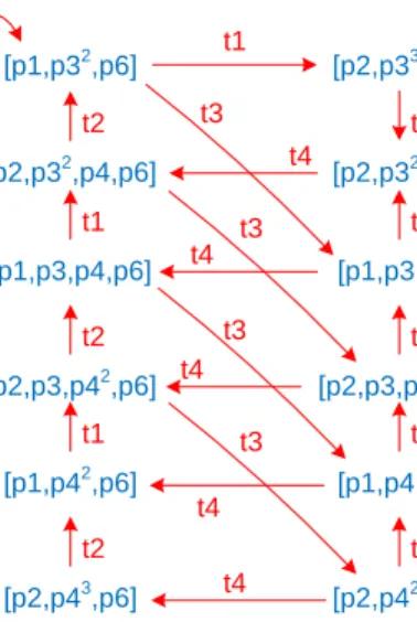
Let (N, M0) be the marked Petri net shown in Figure 3, i.e.,M0= [p1, p32, p6]. The empty sequence σ =h i is enabled in (N, M0). The sequence σ =ht1, t3i is also enabled and results in marking [p2, p32, p5]. Another possible firing se-quence is σ = ht3, t4, t3, t1, t4, t3, t2, t1i. A marking M is reachable from the initial marking M0 iff there exists a sequence of enabled transitions whose fir-ing leads from M0 toM. The set of reachable markings of (N, M0) is denoted [N, M0i. [p1,p32,p6] t1 [p2,p33,p6] [p2,p32,p4,p6] t2 [p1,p3,p4,p6] t1 [p2,p3,p42,p6] t2 [p1,p42,p6] t1 [p2,p43,p6] t2 [p2,p32,p5] t3 [p1,p3,p5] t1 [p2,p3,p4,p5] t2 [p1,p4,p5] t1 [p2,p42,p5] t2 t3 t4 t4 t4 t4 t4 t3 t3 t3
Fig. 4.The reachability graph of the marked Petri net shown in Figure 3.
For the marked Petri net shown in Figure 3 there are 12 reachable states. These states can be computed using the so-called reachability graph shown in Figure 4. All nodes correspond to reachable markings and each arc corresponds to the firing of a particular transition. Any path in the reachability graph corre-sponds to a possible firing sequence. For example, using Figure 4 is is easy to see thatht3, t4, t3, t1, t4, t3, t2, t1iis indeed possible and results in [p2, p3, p4, p5]. A marked net may be unbounded, i.e., have an infinite number or reachable states. In this case, the reachability graph is infinitely large, but one can still construct the so-called coverability graph [50].
3.3 Workflow Nets
For process discovery, we look at processes that are instantiated multiple times, i.e., the same process is executed for multiple cases. For example, the process of handling insurance claims may be executed for thousands or even millions of claims. Such processes have a clear starting point and a clear ending point. Therefore, the following subclass of Petri nets (WF-nets) is most relevant for process discovery.
Definition 4 (Workflow nets).LetN = (P, T, F)be a Petri net and¯ta fresh identifier not in P∪T.N is a workflow net (WF-net) iff:
1. object creation:P contains an input placei (also called source place) such that•i=∅,
2. object completion:P contains an output placeo(also called sink place) such thato•=∅,
3. connectedness:N¯ = (P, T∪ {¯t}, F∪ {(o,¯t),(¯t, i)})is strongly connected, i.e., there is a directed path between any pair of nodes inN¯.
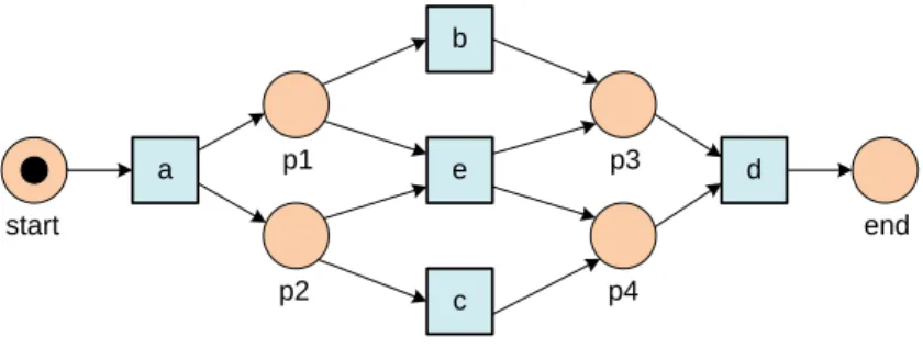
Clearly, Figure 3 is not a WF-net because a source and sink place are missing. Figure 5 shows an example of a WF-net: •start =∅, end• =∅, and every node is on a path from start toend.
a b c d e p2 end p4 p3 p1 start
Fig. 5.A workflow net with source placei=start and sink placeo=end.
The Petri net depicted in Figure 1 is another example of a WF-net. Not every WF-net represents a correct process. For example, a process represented by a WF-net may exhibit errors such as deadlocks, tasks which can never be-come active, livelocks, garbage being left in the process after termination, etc. Therefore, we define the following correctness criterion.
Definition 5 (Soundness). Let N= (P, T, F)be a WF-net with input placei and output placeo.N is soundiff:
1. safeness:(N,[i])is safe, i.e., places cannot hold multiple tokens at the same time,
2. proper completion: for any markingM ∈[N,[i]i,o∈M impliesM = [o], 3. option to complete: for any marking M ∈[N,[i]i,[o]∈[N, Mi, and 4. absence of dead tasks: (N,[i]) contains no dead transitions (i.e., for any
t∈T, there is a firing sequence enabling t).
The WF-nets shown in figures 5 and 1 are sound. Soundness can be veri-fied using standard Petri-net-based analysis techniques. In fact soundness cor-responds to liveness and safeness of the corresponding short-circuited net [1]. This way efficient algorithms and tools can be applied. An example of a tool tailored towards the analysis of WF-nets is Woflan [55]. This functionality is also embedded in our process mining tool ProM [5].
3.4 Problem Definition and Approaches
After introducing events logs and WF-nets, we can define the main goal of pro-cess discovery.
Definition 6 (Process discovery). Let L be an event log over A, i.e., L ∈
IB(A∗). Aprocess discovery algorithmis a functionγ that maps any logLonto a Petri net γ(L) = (N, M). Ideally, N is a sound WF-net and all traces in L correspond to possible firing sequences of(N, M).
The goal is to find a process model that can “replay” all cases recorded in the log, i.e., all traces in the log are possible firing sequences of the discovered WF-net. Assume that L1 = [ha, b, c, di5,ha, c, b, di8,ha, e, di9]. In this case the WF-net shown in Figure 5 is a good solution. All traces inL1correspond to firing sequences of the WF-net and vice versa. Throughout this article, we useL1 as an example log. Note that it may be possible that some of the firing sequences of the discovered WF-net do not appear in the log. This is acceptable as one cannot assume that all possible sequences have been observed. For example, if there is a loop, the number of possible firing sequences is infinite. Even if the model is acyclic, the number of possible sequences may be enormous due to choices and parallelism. Later in this article, we will discuss the quality of discovered models in more detail.
Since the mid-nineties several groups have been working on techniques for process mining [7, 9, 10, 25, 29, 32, 33, 58], i.e., discovering process models based on observed events. In [6] an overview is given of the early work in this domain. The idea to apply process mining in the context of workflow management sys-tems was introduced in [10]. In parallel, Datta [29] looked at the discovery of business process models. Cook et al. investigated similar issues in the context of software engineering processes [25]. Herbst [40] was one of the first to tackle more complicated processes, e.g., processes containing duplicate tasks.
Most of the classical approaches have problems dealing with concurrency. Theα-algorithm [9] is an example of a simple technique that takes concurrency as a starting point. However, this simple algorithm has problems dealing with complicated routing constructs and noise (like most of the other approaches
described in literature). In [32, 33] a more robust but less precise approach is presented.
Recently, people started using the “theory of regions” to process discovery. There are two approaches: state-based regions and language-based regions. State-based regions can be used to convert a transition system into a Petri net [13, 15, 23, 24, 26, 27, 35]. Language-based regions add places as long as it is still possible to replay the log [14, 17, 19, 28, 42, 43].
More from a theoretical point of view, the process discovery problem is related to the work discussed in [12, 37, 38, 49]. In these papers the limits of inductive inference are explored. For example, in [38] it is shown that the computational problem of finding a minimum finite-state acceptor compatible with given data is NP-hard. Several of the more generic concepts discussed in these papers can be translated to the domain of process mining. It is possible to interpret the problem described in this article as an inductive inference problem specified in terms of rules, a hypothesis space, examples, and criteria for successful inference. The comparison with literature in this domain raises interesting questions for process mining, e.g., how to deal with negative examples (i.e., suppose that besides log L there is a log L0 of traces that are not possible, e.g., added by a domain expert). However, despite the relations with the work described in [12, 37, 38, 49] there are also many differences, e.g., we are mining at the net level rather than sequential or lower level representations (e.g., Markov chains, finite state machines, or regular expressions), tackle concurrency, and do not assume negative examples or complete logs.
The above approaches assume that there is no noise or infrequent behav-ior. For approaches dealing with these problems we refer to the work done by Christian G¨unther [39], Ton Weijters [58], and Ana Karla Alves de Medeiros [47].
4
α
-Algorithm
After introducing the process discovery problem and providing an overview of approaches described in literature, we focus on the α-algorithm [9]. The α-algorithm is not intended as a practical mining technique as it has problems with noise, infrequent/incomplete behavior, and complex routing constructs. Never-theless, it provides a good introduction into the topic. The α-algorithm is very simple and many of its ideas have been embedded in more complex and robust techniques. Moreover, it was the first algorithm to really address the discovery of concurrency.
4.1 Basic Idea
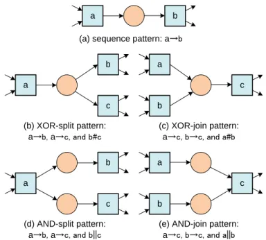
The α-algorithm scans the event log for particular patterns. For example, if activity ais followed by bbut b is never followed by a, then it is assumed that there is a causal dependency between aand b. To reflect this dependency, the corresponding Petri net should have a place connecting ato b. We distinguish four log-based ordering relations that aim to capture relevant patterns in the log.
Definition 7 (Log-based ordering relations).LetLbe an event log overA, i.e., L∈IB(A∗). Let a, b∈A:
– a >L b iff there is a trace σ=ht1, t2, t3, . . . tni andi∈ {1, . . . , n−1} such
thatσ∈L andti =a andti+1=b, – a→Lbiffa >Lb andb6>La,
– a#Lb iffa6>Lb andb6>L a, and
– akLb iffa >Lb andb >L a.
Consider for example L1 = [ha, b, c, di5, ha, c, b, di8, ha, e, di9]. c >L1 d be-cause ddirectly followsc in trace ha, b, c, di. However,d6>L1 c because c never directly follows din any trace in the log.
>L1={(a, b),(a, c),(a, e),(b, c),(c, b),(b, d),(c, d),(e, d)}contains all pairs of activities in a “directly follows” relation. c →L1 d because sometimes d di-rectly follows c and never the other way around (c >L1 d and d 6>L1 c). →L1= {(a, b),(a, c),(a, e),(b, d),(c, d),(e, d)} contains all pairs of activities in a “causality” relation. bkL1c because b >L1 c and c >L1 b, i.e, sometimes c follows b and sometimes the other way around. kL1 = {(b, c),(c, b)}. b#L1e because b 6>L1 e and e 6>L1 b. #L1 = {(a, a),(a, d),(b, b),(b, e),(c, c),(c, e), (d, a),(d, d),(e, b), (e, c),(e, e)}. Note that for any log L over A and x, y ∈ A: x→Ly,y→Lx, x#Ly, or xkLy.
a b
(a) sequence pattern: a→b
a b c (b) XOR-split pattern: a→b, a→c, and b#c a b c (c) XOR-join pattern: a→c, b→c, and a#b a b c (d) AND-split pattern: a→b, a→c, and b||c a b c
(e) AND-join pattern:
a→c, b→c, and a||b
The log-based ordering relations can be used to discover patterns in the corresponding process model as is illustrated in Figure 6. If a and b are in sequence, the log will showa >Lb. If afterathere is a choice betweenb andc,
the log will showa→Lb,a→Lc, andb#Lcbecauseacan be followed byband
c, butbwill not be followed bycand vice versa. The logical counterpart of this so-called XOR-split pattern is the XOR-join pattern as shown in Figure 6(b-c). If a→Lc,b→Lc, anda#Lb, then this suggests that after the occurrence of either
aorb,cshould happen. Figure 6(d-e) shows the so-called split and AND-join patterns. If a→L b,a→Lc, and bkLc, then it appears that afterabothb
and c can be executed in parallel (AND-split pattern). Ifa→L c, b→L c, and
akLb, then it appears thatcneeds to synchronizeaandb(AND-join pattern).
Figure 6 only shows simple patterns and does not present the additional conditions needed to extract the patterns. However, the figure nicely illustrates the basic idea.
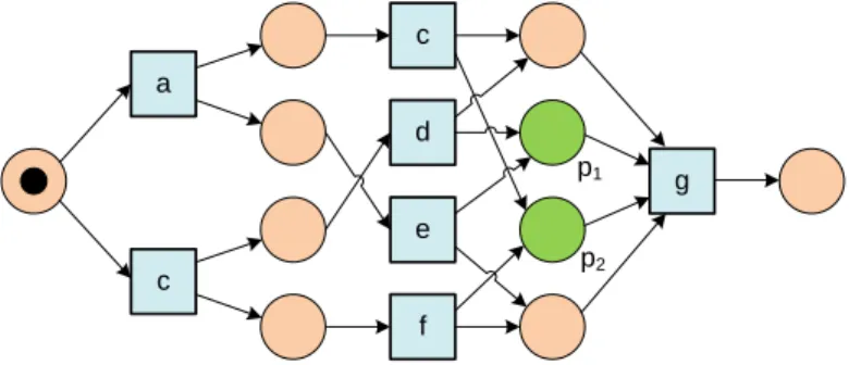
a b c d e p({a,f},{b}) iL p({b},{c}) p({b},{d}) p({c},{e}) p({d},{e}) g oL p({e},{f,g}) f
Fig. 7. WF-net N2 derived from L2 = [ha, b, c, d, e, f, b, d, c, e, gi, ha, b, d, c, e, gi,
ha, b, c, d, e, f, b, c, d, e, f, b, d, c, e, gi].
Consider for example WF-netN2depicted in Figure 7 and the log event log L2= [ha, b, c, d, e, f, b, d, c, e, gi,ha, b, d, c, e, gi,
ha, b, c, d, e, f, b, c, d, e, f, b, d, c, e, gi]. The α-algorithm constructs WF-net N2 based on L2. Note that the patterns in the model indeed match the log-based ordering relations extracted from the event log. Consider for example the process fragment involving b, c, d, and e. Obviously, this fragment can be constructed based onb→L2 c, b→L2 d,ckL2d, c→L2 e, andd→L2 e. The choice following eis revealed bye→L2 f,e→L2 g, andf#L2g. Etc.
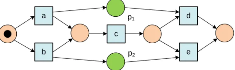
Another example is shown in Figure 8. WF-net N3 can be derived from L3 = [ha, c, di45,hb, c, di42,ha, c, ei38,hb, c, ei22]. Note that here there are two start and two end activities. These can be found easily by looking for the first and last activities in traces.
4.2 Algorithm
b c p({a,b},{c}) oL a iL e d p({c},{d,e})
Fig. 8.WF-netN3 derived fromL3= [ha, c, di45,hb, c, di42,ha, c, ei38,hb, c, ei22].
Definition 8 (α-algorithm).Let Lbe an event log overT.α(L)is defined as follows. 1. TL={t∈T | ∃σ∈L t∈σ}, 2. TI ={t∈T | ∃σ∈L t=first(σ)}, 3. TO ={t∈T | ∃σ∈L t=last(σ)}, 4. XL={(A, B)|A⊆TL ∧ A6=∅ ∧ B⊆TL ∧ B6=∅ ∧ ∀a∈A∀b∈B a→L b ∧ ∀a1,a2∈A a1#La2 ∧ ∀b1,b2∈B b1#Lb2}, 5. YL={(A, B)∈XL | ∀(A0,B0)∈XLA⊆A0 ∧B ⊆B0 =⇒(A, B) = (A0, B0)}, 6. PL={p(A,B) |(A, B)∈YL} ∪ {iL, oL},
7. FL={(a, p(A,B))|(A, B)∈YL ∧ a∈A} ∪ {(p(A,B), b)|(A, B)∈YL ∧b∈
B} ∪ {(iL, t) |t∈TI} ∪ {(t, oL)| t∈TO}, and
8. α(L) = (PL, TL, FL).
Lis an event log over some setT of activities. In Step 1 it is checked which activities do appear in the log (TL). These will correspond to the transitions of
the generated WF-net. TI is the set of start activities, i.e., all activities that
appear first in some trace (Step 2).TO is the set of end activities, i.e., all
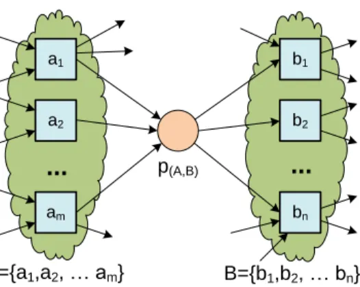
activ-ities that appear last in some trace (Step 3). Steps 4 and 5 form the core of the α-algorithm. The challenge is to find the places of the WF-net and their connec-tions. We aim at constructing places namedp(A,B)such thatAis the set of input transitions (•p(A,B)=A) andB is the set of output transitions (p(A,B)•=B).
The basic idea for findingp(A,B)is shown in Figure 9. All elements ofAshould have causal dependencies with all elements of B, i.e., for any (a, b) ∈ A×B: a →L b. Moreover, the elements of A should never follow any of the other
elements, i.e., for anya1, a2∈A:a1#La2. A similar requirement holds forB. Let us considerL1= [ha, b, c, di5,ha, c, b, di8,ha, e, di9]. ClearlyA={a} and B={b, e}meet the requirements stated in Step 4. Also note thatA0 ={a}and B0 ={b} meet the same requirements.XL is the set of all such pairs that meet
the requirements just mentioned. In this case, XL1 = {({a},{b}),({a},{c}), ({a},{e}),({a},{b, e}),({a},{c, e}),({b},{d}),({c},{d}),({e},{d}),
({b, e},{d}),({c, e},{d})}. If one would insert a place for any element in XL1 there would be too many places. Therefore, only the “maximal pairs” (A, B) should be included. Note that for any pair (A, B)∈XL, non-empty setA0 ⊆A,
and non-empty setB0 ⊆B, it is implied that (A0, B0)∈XL. In Step 5 all
non-maximal pairs are removed. SoYL1 ={({a},{b, e}),({a},{c, e}),({b, e},{d}), ({c, e},{d})}.
a1
...
a2 am b1 b2 bn p(A,B)...
A={a1,a2, … am} B={b1,b2, … bn}Fig. 9.Placep(A,B)connects the transitions in setAto the transitions in setB.
Every element of (A, B)∈YL corresponds to a placep(A,B)connecting tran-sitionsAto transitionsB. In additionPLalso contains a unique source placeiL
and a unique sink placeoL (cf. Step 6).
In Step 7 the arcs are generated. All start transitions in TI have iL as an
input place and all end transitionsTO haveoLas output place. All placesp(A,B) haveA as input nodes andB as output nodes. The result is a Petri net α(L) = (PL, TL, FL) that describes the behavior seen in event logL.
Thus far we presented three logs and three WF-nets. Clearly α(L2) = N2, andα(L3) =N3. In figures 7 and 8 the places are named based on the setsYL2 and YL3. Moreover, α(L1) = N1 modulo renaming of places (because different place names are used in Figure 5). These examples show that the α-algorithm is indeed able to discover WF-nets based event logs.
b p({a},{e}) oL a iL c e f d p({e},{f}) p({b},{c,f}) p({a,d},{b}) p({c},{d})
Fig. 10. WF-net N4 derived from L4 = [ha, b, e, fi2, ha, b, e, c, d, b, fi3,
ha, b, c, e, d, b, fi2
,ha, b, c, d, e, b, fi4
,ha, e, b, c, d, b, fi3
Figure 10 shows another example. WF-net N4 can be derived from L4 = [ha, b, e, fi2,ha, b, e, c, d, b, fi3,ha, b, c, e, d, b, fi2,ha, b, c, d, e, b, fi4,
ha, e, b, c, d, b, fi3], i.e.,α(L
4) =N4.
The WF-net in Figure 1 is discovered when applying theα-algorithm to the event log in the same figure.
4.3 Limitations
In [9] it was shown that the α-algorithm is able to discover a large class of WF-nets if one assumes that the log is complete with respect to the log-based ordering relation>L. This assumption implies that, for any event logL,a >Lb
ifacan be directly followed byb. We revisit the notion of completeness later in this article. g a c d e f c p1 p2
Fig. 11.WF-netN5derived fromL5= [ha, c, e, gi2,ha, e, c, gi3,hb, d, f, gi2,hb, f, d, gi4].
Even if we assume that the log is complete, theα-algorithm has some prob-lems. There are many different WF-nets that have the same possible behavior, i.e., two models can be structurally different but trace equivalent. Consider for exampleL5= [ha, c, e, gi2,ha, e, c, gi3,hb, d, f, gi2,hb, f, d, gi4].α(L5) is shown in Figure 11. Although the model is able to generate the observed behavior, the resulting WF-net is needlessly complex. Two of the input places of g are re-dundant, i.e., they can be removed without changing the behavior. The places denoted as p1 and p2 are so-called implicit places and can be removed without allowing for more traces. In fact, Figure 11 shows only one of many possible trace equivalent WF-nets.
The originalα-algorithm has problems dealing with short loops, i.e., loops of length 1 or 2. This is illustrated by WF-netN6 in Figure 12 which shows the result of applying the basic algorithm toL6= [ha, ci2,ha, b, ci3,ha, b, b, ci2]. It is easy to see that the model does not allow forha, ciandha, b, b, ci. In fact, inN6, transition b needs to be executed precisely once and there is an implicit place connectingaandc. This problem can be addressed easily as shown in [46]. Using an improved version of the α-algorithm one can discover the WF-net shown in Figure 13.
a c b
Fig. 12.Incorrect WF-netN6 derived fromL6= [ha, ci2,ha, b, ci3,ha, b, b, ci2].
a c
b
Fig. 13.WF-netN7 having a so-called “short-loop”.
A more difficult problem is the discovery of so-called non-local dependen-cies resulting from non-free choice process constructs. An example is shown in Figure 14. This net would be a good candidate after observing for example L8 = [ha, c, di45,hb, c, ei42]. However, the α-algorithm will derive the WF-net without the place labeled p1 and p2. Hence,α(L8) =N3 shown in Figure 8 al-though the tracesha, c, eiandhb, c, dido not appear in L8. Such problems can be (partially) resolved using refined versions of theα-algorithm such as the one presented in [59]. b c a e d p1 p2
Fig. 14.WF-netN8 having a non-local dependency.
The above examples show that the α-algorithm is able to discover a large class of models. The basic 8-line algorithm has some limitations when it comes to particular process patterns (e.g., short-loops and non-local dependencies). Some of these problems can be solved using various refinements. However, several more fundamental problems remain as shown next.
5
Challenges
Theα-algorithm was one of the first process discovery algorithms to adequately capture concurrency. Today there are much better algorithms that overcome the weaknesses of theα-algorithm. These are either variants of theα-algorithm or algorithms that use a completely different approach, e.g., genetic mining or synthesis based on regions [34]. Later we will describe some of these approaches. However, first we discuss the main requirements for a good process discovery algorithm.
To discover a suitable process model it is assumed that the event log contains arepresentative sample of behavior. There are two related phenomena that may make an event log less representative for the process being studied:
– Noise:the event log contains rare and infrequent behavior not representative for the typical behavior of the process.
– Incompleteness: the event log contains too few events to be able to discover some of the underlying control-flow structures.
Often we would like to abstract from noise when discovering a process. This does not mean that noise is not relevant. In fact, the goal of conformance check-ing is to identify exceptions and deviations. However, for process discovery it makes no sense to include noisy behavior in the model as this will clutter the diagram and has little predictive value. Whereas noise refers to the problem of having “too much data” (describing rare behavior), completeness refers to the problem of having “too little data”. To illustrate the relevance of completeness, consider a process consisting of 10 activities that can be executed in parallel and a corresponding log that contains information about 10,000 cases. The total number of possible interleavings in the model with 10 concurrent activities is 10! = 3,628,800. Hence, it is impossible that each interleaving is present in the log as there are fewer cases (10,000) than potential traces (3,628,800). Even if there are 3,628,800 cases in the log, it is extremely unlikely that all possible variations are present. For the process in which 10 activities can be executed in parallel, a local notion of completeness can reduce the required number of observations dramatically. For example, for the α-algorithm only 10×(10−1) = 90 rather than 3,628,800 different observations are needed to construct the model.
Completeness and noise refer to qualities of the event log and do not say much about the quality of the discovered model. Determining the quality of a process mining result is difficult and is characterized by many dimensions. As shown in Figure 15, we identify four main quality dimensions:fitness,simplicity, precision, andgeneralization [2, 4, 51].
A model with goodfitness allows for the behavior seen in the event log. A model has a perfect fitness if all traces in the log can be replayed by the model from beginning to end. There are various ways of defining fitness. It can be defined at the case level, e.g., the fraction of traces in the log that can be fully replayed. It can also be defined at the event level, e.g., the fraction of events in the log that are indeed possible according to the model [2, 4, 51]. Note that we defined an event log to be a multi-set of traces rather than an ordinary set:
process discovery
fitness
precision
generalization
simplicity
“able to replay event log” “Occam’s razor”
“not overfitting the log” “not underfitting the log”
Fig. 15.Balancing the four quality dimensions:fitness,simplicity,precision, and gen-eralization[2].
the frequencies of traces are important for determining fitness. If a trace cannot be replayed by the model, then the significance of this problem depends on the relative frequency.
Thesimplicitydimension in Figure 15 refers toOccam’s Razor, the principle that states that “one should not increase, beyond what is necessary, the number of entities required to explain anything”. Following this principle, we look for the “simplest process model” that can explain what is observed in the event log. The complexity of the model could be defined by the number of nodes and arcs in the underlying graph. Also more sophisticated metrics can be used, e.g., metrics that take the “structuredness” or “entropy” of the model into account.
Fitness and simplicity are obvious criteria. However, this is not sufficient as will be illustrated using Figure 16. Assume that the four models that are shown are discovered based on the event log also depicted in the figure. (Note that this event log was already shown in Section 1.) There are 1391 cases. Of these 1391 cases, 455 followed the traceha, c, d, e, hi. The second most frequent trace isha, b, d, e, giwhich was followed by 191 cases.
If we apply theα-algorithm to this event log, we obtain modelN1 shown in Figure 16. A comparison of the WF-netN1and the log shows that this model is quite good; it is simple and has a good fitness. WF-netN2models only the most frequent trace, i.e., it only allows for the sequence ha, c, d, e, hi. Hence, none of the other 1391−455 = 936 cases fits. WF-netN2is simple but has a poor fitness. Let us now consider WF-net N3, this is a variant of the so-called “flower model” [2, 51], i.e., a model that allows for all known activities at any point in time. Note that a Petri net without any places can replay any log and has a be-havior similar to the “flower model” (but is not a WF-net). Figure 16 does not show a pure “flower model”, but still allows for a diversity of behaviors.N3 cap-tures the start and end activities well. However, the model does not put any con-straints on the other activities. For example traceha, b, b, b, b, b, b, f, f, f, f, f, gi
a start register request b examine thoroughly c examine casually d check ticket decide pay compensation reject request reinitiate request e g h f end a start register request c examine casually d check ticket decide reject request e h end
N3 : fitness = +, precision = -, generalization = +, simplicity = +
N2 : fitness = -, precision = +, generalization = -, simplicity = + a start register request b examine thoroughly c examine casually d check ticket decide pay compensation reject request reinitiate request e g h f end
N1 : fitness = +, precision = +, generalization = +, simplicity = +
a start register request c examine casually d check ticket decide reject request e h end
N4 : fitness = +, precision = +, generalization = , simplicity = -a register request d examine casually c check ticket decide reject request e h a c examine casually d check ticket decide e g a d examine casually c check ticket decide e g register request register request pay compensation pay compensation a register request b d check ticket decide reject request e h a register request d b check ticket decide reject request e h a b d check ticket decide e g register request pay compensation examine thoroughly examine thoroughly examine thoroughly
…
(all 21 variants seen in the log)acdeh abdeg adceh abdeh acdeg adceg adbeh acdefdbeh adbeg acdefbdeh acdefbdeg acdefdbeg adcefcdeh adcefdbeh adcefbdeg acdefbdefdbeg adcefdbeg adcefbdefbdeg adcefdbefbdeh adbefbdefdbeg adcefdbefcdefdbeg 455 191 177 144 111 82 56 47 38 33 14 11 9 8 5 3 2 2 1 1 1 # trace 1391
is possible, whereas it seems unlikely that this trace is possible when looking at the event log, i.e., the behavior is very different from any of the traces in the log.
Extreme models such as the “flower model” (anything is possible) show the need for an additional dimension: precision. A model is precise if it does not allow for “too much” behavior. Clearly, the “flower model” lacks precision. A model that is not precise is “underfitting”. Underfitting is the problem that the model over-generalizes the example behavior in the log, i.e., the model allows for behaviors very different from what was seen in the log.
WF-netN4 in Figure 16 reveals another potential problem. This model sim-ply enumerates the 21 different traces seen in the event log. Note that N4 is a so-called labeled Petri net, i.e., multiple transitions can have the same label (there are 21 transition with labela). The WF-net in Figure 16 is precise and has a good fitness. However,N4is also overly complex and is “overfitting”. WF-net N4 illustrates the need to generalize; one should not restrict behavior to the traces seen in the log as these are just examples. Overfitting is the problem that a very specific model is generated whereas it is obvious that the log only holds example behavior, i.e., the model explains the particular sample log, but a next sample log of the same process may produce a completely different process model. Recall that logs are typically far from complete. Moreover, generalization can be used to simplify models. WF-net N1 shown in Figure 16 allows for be-havior not seen in the log, e.g.,ha, d, c, e, f, d, b, e, f, c, d, e, hi. Any WF-net that restricts the behavior to only seen cases will be much more complex and exclude behavior which seems likely based on similar traces in the event log.
For real-life event logs it is challenging to balance the four quality dimensions shown in Figure 15. For instance, an oversimplified model is likely to have a low fitness or lack of precision. Moreover, there is an obvious trade-off between underfitting and overfitting [2, 4, 48, 51].
6
Process Discovery and the Theory of Regions
Problems similar to process discovery arise in other areas ranging from hardware design and to controller synthesis of manufacturing systems. Often the so called theory of regionsis used to construct a Petri net from a behavioral specification (e.g., a language or a state space), such that the behavior of this net corresponds to the specified behavior (if such a net exists). The general question answered by the theory of regions is:Given the specified behavior of a system, what is the Petri net that represents this behavior?.
Two main types of region theory can be distinguished, namelystate-based region theoryandlanguage-based region theory. The state-based theory of regions focusses on the synthesis of Petri nets from state-based models, where the state space of the Petri net is bisimilar to the given state-based model. The language-based region theory, considers a language over a finite alphabet as a behavioral specification. Using the notion of regions, a Petri net is constructed, such that all words in the language are firing sequences in that Petri net.
The aim of the theory of regions is to synthesize a precise model, with mini-mal generalization, while keeping a maximini-mal fitness. The classical approaches de-scribed in this section (i.e., conventionalstate-based region theory andlanguage based region theory) do not put much emphasis on simplicity. Unlike algorithms such as the heuristic miner [58], the genetic miner [47], and the fuzzy miner [39], conventional region-based methods do not compromise on precision in favor of simplicity or generalization.
In the remainder of this section, we introduce the main region theory concepts and discuss the differences between synthesis and process discovery. In Section 7 and Section 8 we show how region theory can be used in the context of process discovery.
6.1 State Based Region Theory
The state-based region theory [13, 15, 23, 24, 26, 27, 35] uses a transition system as input, i.e., it attempts to construct a Petri net that is bisimilar to the transi-tion system. Hence both are behaviorally equivalent and if the system exhibits concurrency, the Petri net may be much smaller than the transition system. Definition 9 (Transition system). T S = (S, E, T) defines a labeled tran-sition system where S is the set of states, A is the set of visible activities (i.e., activities recorded in event log), τ 6∈ A is used to represent silent steps (i.e., actions not recorded in event log), E = A∪ {τ} is the set of transi-tion labels, and T ⊆ S ×E ×S is the transition relation. We use s1
e → s2 to denote a transition from state s1 to s2 labeled with e. Furthermore, we say that Ss = {s ∈ S | 6 ∃
s0∈S,e∈E s0 e
→ s} ⊆ S is the set of initial states, and Se={s∈S| 6 ∃s0∈S,e∈E s
e
→s0} ⊆S is the set of final states.
In the transition system, aregion corresponds to a set of states such that all states have similarly labeled input and output edges. Figure 17 shows an example of a transition system. In fact, this figure depicts the reachability graph of the Petri net in Figure 5, where the states are anonymous, i.e., they do not contain information about how many tokens are in a place.
Definition 10 (State region). LetT S= (S, E, T)be a transition system and S0 ⊆S a set of states. We sayS0 is a region, if and only if for alle∈E one of the following conditions holds:
1. all the transitionss1
e
→s2 enterS0, i.e., s1∈/ S0 ands2∈S0, 2. all the transitionss1
e
→s2 exit S0, i.e., s1∈S0 ands2∈/S0, 3. all the transitionss1
e
→s2 do not crossS0, i.e.,s1, s2∈S0 ors1, s2∈/ S0 Any transition systemT S = (S, E, T) has two trivial regions:∅ (the empty region) and S (the region consisting of all states). Typically, only non-trivial regions are considered. A region r0 is said to be asubregion of another regionr ifr0 ⊂r. A regionrisminimal if there is no other regionr0which is a subregion of r. Region r is a preregion of e if there is a transition labeled with e which
s1 a s2 c s3 s5 b s6 c s7 d s4 d s8 e b
Fig. 17.A transition system with 8 states, 5 labels, 1 initial state and 2 final states.
s1 a s2 c s3 s5 b s6 c s7 d s4 d s8 e b a b c d e p1 p2 p3 p4 p5 p6
Fig. 18. The transition system of Figure 17 is converted into a Petri net using the “state regions”. The six regions correspond to places in the Petri net.
(classical region theory) s1 a s2 d s4 s3 e d a d e p1 p2 p3 a d1 e p1 p2 p4 d2 p3 (using label splitting)
Fig. 19.The transition system is not elementary. Therefore, the generated Petri net using classical region theory is not equivalent (modulo bisimilarity). However, using “label-splitting” an equivalent Petri net can be obtained.
exitsr. Regionris apostregionofeif there is a transition labeled withewhich entersr.
For Petri net synthesis, a region corresponds to a Petri net place and an event corresponds to a Petri nettransition. Thus, the main idea of thesynthesis algorithm is the following: for each eventein the transition system, a transition labeled witheis generated in the Petri net. For each minimal regionria placepi
is generated. The flow relation of the Petri net is built the following way:e∈pi•
if ri is a preregion of e and e∈ •pi if ri is a postregion of e. Figure 18 shows
the minimal regions of the transition system of Figure 17 and the corresponding Petri net.
The first publications on the theory of regions only dealt with a special class of transition systems called elementary transition systems. See [13, 15, 30] for details. The class of elementary transition systems is very restricted. In practice, most of the time, people need to deal with arbitrary transition systems that only by coincidence fall into the class of elementary transition systems. In the papers of Cortadella et al. [26, 27], a method for handling arbitrary transition systems was presented. This approach useslabeled Petri nets, i.e., different transitions can refer to the same event. (WF-netN4in Figure 16 is an example of a labeled Petri net, e.g., there are 21 transitions labeleda.) For this approach it has been shown that the behavior (cf. reachability graph) of the synthesized Petri net isbisimilar to the initial transition system even if the transition system is non-elementary.
More recently, in [23,24], an approach was presented where the constructed Petri net is not necessarily safe, but bounded1. Again, the reachability graph of the synthesized Petri net is bisimilar to the given transition system.
To illustrate the problem of non-elementary transition systems, consider Fig-ure 19. This transition system is not elementary. The problem is that there are two statess2 ands3 that are identical in terms of regions, i.e., there is no region such that one is part of it and the other is not. As a result, the constructed Petri net on the left hand side of Figure 19 fails to construct a bisimilar Petri net. However, using label-splitting as presented in [26, 27], the Petri net on the right hand side can be obtained. This Petri net has two transitions d1 andd2 corre-sponding to activitydin the log. The splitting is based on the so-called notions of excitation and generalized excitation region, see [26]. As shown in [26, 27] it is always possible to construct an equivalent Petri net. However, label-splitting may lead to larger Petri nets. In [21] the authors show how to obtain the most precise model when label splitting is not allowed.
In state-based region theory, the aim is to construct a Petri net, such that its behavior is bisimilar to the given transition system. In process discovery however, we have a log as input, i.e., we have information about sequences of transitions, but not about states. In Section 7, we show how we can identify state information from event logs and then use state-based region theory for process discovery. However, we first introduce language-based region theory.
6.2 Language Based Region Theory
In addition to state-based region theory, we also consider language-based region theory [14, 17, 19, 28, 42, 43]. In their survey paper [45], Mauser and Lorenz show how for different classes of languages (step languages, regular languages and (infinite) partial languages) a Petri net can be derived such that the resulting net is the Petri net with the smallest behavior in which the words in the language are possible firing sequences.
Given a prefix-closed languageAover some non-empty, finite set of activities A, the language-based theory of regions tries to find a finite Petri net N(A) in which the transitions correspond to the elements in the set A and of which all sequences in the language are firing sequences (fitness criterion). Furthermore, the Petri net should minimize the number of firing sequences not in the language (precision criterion).
The Petri net N(A) = (∅, A,∅) is a finite Petri net with infinitely many firing sequences allowing for any sequence involving activitiesA. Such a model is typically underfitting, i.e., allowing for more behavior than suggested by the event log. Therefore, the behavior of this Petri net needs to be reduced so that the Petri net still allows to reproduce all sequences in the language, but does not allow for behavior unrelated to the examples seen in the event log. This is achieved by adding places to the Petri net. The theory of regions provides a method to identify these places, usinglanguage regions.
1
A Petri net is safe if there can never be more than 1 token in any place. Boundedness implies that there exists an upper bound for the number of tokens in any place.
Definition 11 (Language Region). Let A be a set of activities. A region of a prefix-closed language L overA is a triple (~x, ~y, c) with~x, ~y∈ {0,1}A and
c∈ {0,1}, such that for each non-empty sequencew=w0◦a∈ L,w0∈ L,a∈A: c+X
t∈A
~
w0(t)·~x(t)−w(t)~ ·~y(t)≥0
This can be rewritten into the inequation system: c·~1 +M0·x~−M·~y≥~0
whereM andM0are two|L|×|A|matrices withM(w, t) =w(t), and~ M0(w, t) = ~
w0(t), with w=w0◦a. The set of all regions of a language is denoted by <(L)
and the region(~0, ~0,0)is called the trivial region.2
Consider a regionr= (~x, ~y, c) corresponding to some placepr. For any prefix
w=w0◦ainL, regionrsatisfiesc+P t∈A
~
w0(t)·~x(t)−w(t)~ ·~y(t)≥0 where
c is the initial number of tokens in place pr, Pt∈A w~0(t)·~x(t) is the number
of tokens produced for place pr just before firing a (note that w0 is the prefix
without including the last a), and P
t∈A w(t)~ ·~y(t) is the number of tokens
consumed from placepr after firinga(wis the concatenation ofw0 anda).w~ is
the Parikh vector of w, i.e.,w(t) is the number of times~ t appears in sequence w. ~x(t) is the number of tokens t produces for placepr. Transitiont consumes
~
y(t) tokens from placeprper firing. So,w(t)~ ·~y(t) is the total number of tokens
t consumes from placepr when executingw.
t
1t
2t
4t
3 x1 x2 x3 x4 y1 y2 y3 y2c
Fig. 20.Region for a language with four letters:t1,t2,t3, andt4.
Figure 20 illustrates the language-based region concept using for a language over four activities (|A|=4), i.e., each solution (~x, ~y, c) of the inequation system can be regarded in the context of a Petri net, where the region corresponds to a
2
To reduce calculation time, the inequation system can be rewritten to the form [~1;M0;−M]·~r≥~0 which can be simplified by eliminating duplicate rows.
feasible place with preset {t|t∈T, ~x(t)≥1} and postset{t|t∈T, ~y(t)≥1}, and initially marked with c tokens. In this paper, we assume arc-weights to be 0 or 1 as we aim at understandable models (i.e.,~x, ~y ∈ {0,1}A). As shown
in [14, 16, 28, 43] it is possible to generalize the above notions to arbitrary arc-weights.
A place represented by a region can be added to a Petri net, without limiting its behavior with respect to traces seen in the event log. Therefore, we call such a placefeasible.
Definition 12 (Feasible place).LetLbe a prefix-closed language overAand let N = ((P, T, F), M) be a marked Petri net with T =A and M ∈IB(P). A place p∈P is called feasible if and only if there exists a corresponding region (~x, ~y, c) ∈ <(L) such that M(p) = c, and ~x(t) = 1 if and only if t ∈ •p, and
~
y(t) = 1 if and only ift∈p•.
In [16, 43] it was shown that any solution of the inequation system of Defini-tion 11 can be added to a Petri net without influencing the ability of that Petri net to replay the log. However, since there are infinitely many solutions of that inequation system (assuming arc weights), there are infinite many feasible places and the authors of [16, 43] present two ways of finitely representing these places, namely abasis representation [43] and aseparating representation [16, 43].
6.3 Process Discovery vs. Region Theory
When comparing region theory—state-based or language based—with process discovery, some important differences should be noted. First of all, in region theory, the starting point is afull behavioral specification, either in the form of a (possibly infinite) transition system, or a (possibly infinite) language. Hence, the underlying assumption is that the input iscomplete andnoise free and therefore maximal fitness is assured.
Second, the aim of region theory is to provide acompact, exact representation of that behavior in the form of a Petri net. If the net allows for more behavior than specified, then this additional behavior can be proven to be minimal, hence region theory providesprecise results.
Finally, when region theory is directly applied in the context of process dis-covery [16, 21, 53], the resulting Petri nets typically perform poorly with respect to two of the four dimensions shown in Figure 15. The resulting models are typically overfitting (lack of generalization) and are too difficult to comprehend (simplicity criterion). Therefore, in sections 7 and 8, we show how region theory can be modified for process discovery. The key idea is to allow the algorithms to generalize and relax on preciseness, with the aim of obtaining simpler models.
7
Process Discovery Using State-Based Region Theory
In Section 2 we introduced the concept of control-flow discovery and discussed the problems of existing approaches. In Section 6, we introduced region theoryand showed the main differences with control flow discovery. In this section, we introduce a two-step approach to combine process discovery with state-based region theory [8]. In the remainder, we elaborate on these two steps and discuss challenges.
7.1 From Event Logs to Transition Systems
In the first step, we construct a transition system from the log, where we gener-alize from the observed behavior. Furthermore, we “massage” the output, such that the region theory used in the second step is more likely to produce a simple model. In the second step, we use classical state-based region theory to obtain a Petri net. This section describes the first and most important step. Depending on the desired properties of the model and the characteristics of the log, the algorithm can be tuned to provide a more simple and/or generic model.
The most important aspect of process discovery isdeducing the states of the operational process in the log. Most mining algorithms have an implicit notion of state, i.e., activities are glued together in some process modeling language based on an analysis of the log and the resulting model has a behavior that can be represented as a transition system. In this section, we propose to define states explicitly and start with the definition of a transition system.
trace:
a b c d c d c d e f a g h h h i
past
future
current state
past and future
Fig. 21. Three basic “ingredients” can be considered as a basis for calculating the “process state”: (1) past, (2) future, and (3) past and future.
In some cases, the state can be derived directly, e.g., each event encodes the complete state by providing values for all relevant data attributes. However, in the event log we typically only see activities and not states. Hence, we need to deduce the state information from the activities executed before and after a given state. Based on this, there are basically three approaches to defining the state of a partially executed case in a log:
– past, i.e., the state is constructed based on the history of a case, – future, i.e., the state of a case is based on its future, or
abcd acbd aed abcd abcd aed acbd ...
(b) transition system based on postfix
<> a <a> e <a,e> d <a,e,d> <a,b> b <a,b,c> c <a,b,c,d> d
<a,c> b <a,c,b> d <a,c,b,d> c <a,b,c,d> a <b,c,d> <a,e,d> <e,d> <a,c,b,d> a a <c,b,d> <d> e <c,d> <b,d> b c c b <> d <> <a,b,c,d> a <a> <b,c,d> <> <a,e,d> <a> <e,d> <> <a,c,b,d> a a <a> <c,b,d> <a,e> <d> e <a,b> <c,d> <a,c> <b,d> b c <a,e,d> <> d <a,c,b> <d> b <a,b,c> <d> c <a,b,c,d> <> d <a,c,b,d> <> d
(c) transition system based on prefix and postfix (a) transition system based on prefix
Fig. 22. Three transition systems derived from the logL1 = [ha, b, c, di5,ha, c, b, di8,
ha, e, di9
].
Figure 21 shows anexample of a trace and the three different “ingredients” that can be used to calculate state information. Given a concrete trace, i.e., the execution of a case from beginning to end, we can look at the state after executing the first nine activities. This state can be represented by the prefix, the postfix, or both.
To explain the basic idea of constructing a transition system from an event log, consider Figure 22. If we just consider the prefix (i.e., the past), we get the transition system shown in Figure 22(a). Note that the initial state is denoted
hi, i.e., the empty sequence. Starting from this initial state the first activity is always ain each of the traces. Hence, there is one outgoing arc labeleda, and the subsequent state is labeledhai. From this state, three transitions are possible
![Fig. 15. Balancing the four quality dimensions: fitness, simplicity, precision, and gen- gen-eralization [2].](https://thumb-us.123doks.com/thumbv2/123dok_us/370346.2540783/21.918.258.667.185.388/fig-balancing-quality-dimensions-fitness-simplicity-precision-eralization.webp)
