Targeted Methods for Finding Quantitative Trait Loci

University of California, Berkeley

U.C. Berkeley Division of Biostatistics Working Paper Series

Year  Paper

Targeted Methods for Finding Quantitative

Trait Loci

Hui Wang

Sherri Rose

Mark J. van der Laan

∗_{Stanford University, [email protected]}

†_{University of California, Berkeley, [email protected]} ‡_{University of California, Berkeley, [email protected]}

This working paper is hosted by The Berkeley Electronic Press (bepress) and may not be commer-cially reproduced without the permission of the copyright holder.

http://biostats.bepress.com/ucbbiostat/paper285 Copyright c2011 by the authors.

Targeted Methods for Finding Quantitative

Trait Loci

Hui Wang, Sherri Rose, and Mark J. van der Laan

Abstract

Conventional genetic mapping methods typically assume parametric models with Gaussian errors, and obtain parameter estimates through maximum likelihood es-timation. We propose a general semiparametric model to map quantitative trait loci (QTL) in experimental crosses. In contrast with widely-used interval map-ping (IM) derived methods, our model requires fewer assumptions and also ac-commodates various machine learning algorithms. Estimation using both targeted maximum likelihood and collaborative targeted maximum likelihood methods is compared to a composite interval mapping (CIM) approach. We demonstrate with simulations and real data analyses that, on average, our semiparametric targeted learning approach produces less biased QTL effect estimates than those from para-metric models.

Targeted Methods for Finding Quantitative Trait Loci

Hui Wang, Sherri Rose, and Mark van der Laan

Division of Biostatistics, School of Public Health, University of California, Berkeley, California 94720

1

Introduction

The goal of quantitative trait loci (QTL) mapping is to identify genes underlying an observed trait in the genome using genetic markers. In experimental organisms, the QTL mapping experiment usually involves crossing two inbred lines with substantial differences in a trait, and then scoring the trait in the segregating progeny. A series of markers along the genome is genotyped in the segregating progeny, and associations between the trait and the QTL can be evaluated using the marker information. Of primary interest are the positions and effect sizes of QTL genes.

Early literature (Sax 1923; Thoday 1960) focused on directly analyzing a single marker using analysis of variance (ANOVA). The biggest disadvantage of such marker-based analysis is its in-ability to assess QTL genes between markers. In 1989, Lander and Botstein proposed the interval mapping (IM) method (Lander and Botstein 1989). With IM, the genotypic value of a QTL fol-lows a multinomial distribution, determined by the distance of the QTL to its flanking markers and the genotypes of the flanking markers. The trait value is modeled as a Gaussian mixture with the mixing proportions being the multinomial probabilities of the QTL genotype. The significance of the QTL effect is then assessed using likelihood ratio test. By testing positions at small increments along the genome, a whole-genome finely scaled test statistic profile can be constructed. IM has greatly increased the accuracy of estimating QTL parameters, and it has gained wide popularity in the genetic mapping community. Later, Haley and Knott developed a regression method to ap-proximate IM (Haley and Knott 1992). This method imputes the unobserved genotypic value of a putative QTL with its expected value.

IM methods unrealistically assume there is only one gene underlying the observed trait in the entire genome, represented as testing each potential position separately (Lander and Botstein 1989) or computing the univariate association between the expected genotypic value and the phenotypic trait in Haley–Kott regression. In other words, IM only considers the current QTL; all other QTL genes are ignored. When this assumption is violated, the effects of other QTL genes are contained within the residual variance, affecting the assessment of QTL parameters.

To handle multiple QTL genes, Jansen (1993) and Zeng (1994) developed a composite inter-val mapping (CIM) approach. In CIM, background markers are added to a standard IM statistical model to reduce noise and increase the precision of QTL effect estimates. Thus, the CIM approach estimates QTL effects adjusted for confounding markers and can substantially improve the perfor-mance of IM when the background markers are properly chosen. Multiple interval mapping (MIM) was also developed to simultaneously estimate effects and positions of multiple QTL genes (Kao et al. 1999). MIM enjoys greater power but is computationally difficult. It also has a long-standing estimator selection problem: Which QTL genes are to be included? Bayesian approaches have also been studied and applied in QTL mapping (Satagopan et al. 1996; Heath 1997; Sillanpaa and Arjas 1998).

In recent years, with finely scaled single nucleotide polymorphism (SNP) markers replacing the traditional widely spaced microsatellite markers, identifying QTL genes between markers has become less concerning. Due to the high-dimensional nature of SNP data, the univariate marker-trait regression is widely used for its simplicity and computational feasibility despite its noisy results.

Machine learning algorithms, such as random forests (Breiman 2001), are also used to map QTL genes (Lee et al. 2008). While machine learning algorithms are powerful statistical tools, their

use in QTL mapping is limited. These algorithms are particularly good at identifying interactions between genes and predicting the conditional expectation of the outcome given the covariates (in our case, genetic markers). However, their variable importance measurements (VIMs) lack p -values and are otherwise not targeted toward the effects of interest.

Many of the QTL methods discussed above are fully parametric and typically assume a Gaus-sian distribution for the phenotypic trait, as well as require specification of a parametric regression model. The estimation of QTL effects often relies on the method of maximum likelihood estima-tion. Maximum likelihood estimation based on such parametric regression models is widely used and well studied, with software available in many platforms. However, quite often, these paramet-ric models represent an over-simplified description of the underlying genetic mechanism and leads to biased estimates. In addition, if the parametric model is data-adaptively selected among a set of candidate parametric regression models, then the reported standard errors and the p-values are not interpretable.

In this technical report, we address the QTL mapping problem through the use of a semipara-metric regression model, the targeted maximum likelihood estimator (TMLE) (van der Laan and Rubin 2006; van der Laan and Rose 2011) and the collaborative TMLE (C-TMLE) (van der Laan and Gruber 2010; van der Laan and Rose 2011). The only assumption of the semiparametric re-gression model is that the phenotypic trait changes linearly with the QTL gene. We define the TMLE and, in particular, the C-TMLE, which is an appealing estimator for high-dimensional ge-nomic data structures. Our approach allows one to explore a much larger model space with fewer restrictions while still being computational feasible with its incorporation of machine learning al-gorithms. The (C-)TMLE approach targets the VIMs of interest (i.e., the QTL genes) and can provide improved QTL gene effect estimates and rankings by taking advantage of the prediction power of machine learning algorithms. Excerpts from this technical report have been published in the refereed literature (Wang et al. 2010, 2011) with several remaining unpublished sections submitted for publication in a final third paper.

2

Methods

Typical segregating designs include the backcross (B1) design and the intercross (F2) design. Backcross is produced by back crossing the first generation (F1) to one of its parental strains; F2 is produced by intercrossing the first generation (F1 x F1). In a backcross population, there are two possible genotypesAaandaaat any locus; in an F2 population, there are three genotypesAA, Aa, andaa. For the ease of presentation, we will use backcross to demonstrate our method. All the derivations can be readily extended to F2 population and other types of experimental crosses.

2.1

Semiparametric Regression Model

Suppose the observed data are i.i.d. realizations of O_i= (Yi,Mi)∼P0, i=1, . . . ,n, whereY

rep-resents the phenotypic trait value,Mrepresents the marker genotypic values, andiindexes theith subject. Let Abe the genotypic value of the putative QTL under consideration. When A lies on a marker, Ais observed. WhenAlies between markers, it is unobserved. In this case, we impute A with its expected value from a multinomial distribution computed from the genotypes and the

relative locations of its flanking markers. This is the same strategy used in Haley–Knott regression (Haley and Knott 1992), and we will thus only be estimating the effect of an imputed A. The semiparametric regression model for the effect ofAat valueA=arelative toA=0, adjusted for a user-supplied set of other markersM−, is given by

E0(Y |A=a,M−)−E0(Y |A=0,M−) =β0a. (1)

Other parametric forms, such asa∑J_j=1βjVjincorporating effect modification by other markersVj,

can be incorporated as well. We viewβ0as our parameter of interest, which also corresponds with

a marginal average effect obtained by averaging this conditional effect over the distribution ofM−. In a backcross population, when the homozygote aa is coded 0 and the heterozygote Aa is coded 1, β0 measures the effect of the Aa genotype on Y relative to aa. In an F2 population,

with the coding (AA,Aa,aa) = (1,0,−1), β0 can be interpreted as the difference in Y when A

changes from heterozygote to homozygote. In the above model, the only assumption we make is the linearity of the QTL effect (i.e. β0A) on the phenotype. We do not impose any distributional

assumption on the data and any functional form on all functions f(M−) of M−. For β0 to be

estimable and to be well defined, we also need the assumption thatAis not a perfect surrogate of M−. In other words, if we choose to estimate E₀(A|M−), the R2 (coefficient of determination) from the estimator has to be less than 1.

2.2

The TMLE

The TMLE ofβ0(van der Laan and Rubin 2006; Tuglus and van der Laan 2011) involves an initial

machine learning (e.g., super learner) fit of E₀(Y |M) based on the squared error loss function, which yields a fit ofE0(Y|A=0,M−), mapping the latter into an initial estimator ofβ0and thereby

ofE₀(Y |A,M−)in the semiparametric regression model. After obtaining this initial estimator of E₀(Y |A,M−)of the semiparametric form as enforced by the semiparametric regression model, we carry out a single targeted update step by adding an estimate of the clever covariateA−E0(A|M−),

and fitting the coefficient ε in front of this clever covariate with univariate regression, using the

initial estimator ofE₀(Y |A,M−)as offset. Note that the TMLE ofβ0is now simplyβn0+εn. The

TMLE algorithm defined below is performed for eachA.

Obtain an initial estimatorQ0_nforE₀(Y |A,M−). This initial estimator has to respect the

semi-parametric model in equation (1) and takes the formQ0_n=β_n0A+fn(M−).

Obtain a reasonable estimateg_n(W)of the marker confounding mechanismE₀(A|W). We

typ-ically only need to focus on a subsetW ofM−that is viewed as potential confounders of the effect ofAonY. Hence, we can rewrite theg₀(M−)asg₀(W), and we denote its estimator withg_n(W). In our application,W is the set of markers on the same chromosome asA.

Computer(A,W) =A−gn(W). The r(A,W) is the residual of gn(W), also referred to as the

“clever covariate”. It plays the key role of correcting the bias in the initial estimator.

Fit the “ε-regression.” This regression is given byY0∼εr(A,W)whereY0=Y−Q0_n(A,M−)and

Update. The initial estimate ofβ_n0 is updated with β_n1=β_n0+εn, and the initial fitted value Q0n

withQ1_n(A,M−) =Q0_n(A,M−) +εnr(A,W).

Compute the variance estimateσ_n2forβ_n1. Using influence-curve-based methods, we calculate

the variance estimate

σ_n2= ∑i(Yi−Q

1

n(Ai,Mi−))2ri(Ai,Wi)2

(∑iAir(Ai,Wi))2

.

The TMLE estimator will be consistent if either theQ0_nor theg_n(W)is consistent, and will be efficient whenQ0_nis consistent. In other words, whenQ0_nis correctly specified, the TMLE estimate of β essentially stays unchanged with minor modification from the second stage. When Q0_n is

mis-specified, a correct specification of theg_n(W)will achieve a full bias reduction forQ0_nandβ0.

The estimation of the clever covariate requires an estimator ofE0(A|M−)(orE0(A|W)). The

latter can be carried out with a machine learning algorithm regressingAonM−. In particular, one could decide to fit this regression of the marker of interest on two flanking markers, thereby dra-matically simplifying the estimation problem, while potentially capturing most of the confounding by the total marker setM−. The choice of how great the distance between the flanking markers will be is a delicate issue. If one selects the flanking markers right next to the marker of interest, the data might not allow the separation of the effect of interest from the effect of the flanking markers. That is, one is aiming to adjust for confounders that are too predictive of the marker of interest. On the other hand, if one selects the flanking markers too far away from the marker of interest, the flanking markers will not adjust well for the markers that are in between the marker of interest and the flanking markers. Simulations in the previous chapter suggest that the TMLE shows no sign of deterioration for correlations smaller than 0.7 between the marker of interest and the confounders. This could be used to set the window width defined by the two flanking markers. Subject matter considerations, such as that the scientist would be satisfied with a claim that the targeted effect of the marker can be due to other markers in a window of a particular size, could also be used to set this window width of the flanking markers.

An alternative approach is to let the data decide what other markers to include in the model forE₀(A|M−). For that purpose, we can employ the C-TMLE (using a linear regression working model for fluctuation of initial estimator) for estimation of an additive effectE0(E0(Y|A=1,W)− E₀(Y |A=0,W))for the observed data structureO= (W,A,Y)and nonparametric model for the probability distribution P₀ of O. This C-TMLE has also been implemented for this estimation problem, but, obviously, now in terms of TMLEs in this semiparametric regression model. Thus, this algorithm involves using forward selection of main terms to build a main term linear regression fit forE₀(A|M−), based on the sum of squared residuals (i.e., MSE) of the corresponding TMLE of E0(Y |A,M−) that uses this main term regression fit of E0(A|M−) in the clever covariate.

Cross-validation is used to select the number of main terms (i.e., the number of forward selection steps that the algorithm carries out) that will actually be included in the fit of E₀(A|M−). The candidate main terms can include fits of E0(A|M−) such as one based on two flanking markers

defined by a choice of window width, across a number of possible window widths. In this manner the C-TMLE algorithm can data-adaptively decide how aggressive the targeting step should be in its effort to reduce bias due to residual confounding.

The C-TMLE implementation may also involve the selection of a penalty to be added to the MSE in order to make the procedure more robust in the context of having to adjust for highly

cor-related markers. Details are presented in the next section. C-TMLE allows one to data-adaptively determine the markers to include in the fit of E0(A|W). For example, one may wish to only

adjust for the two closest markers that are farther than δ-apart from the marker A, and one can

use C-TMLE to data-adaptively select this choiceδ based on the log-likelihood of the TMLE of

the semiparametric regression fit. In our simulations and data analysis we have implemented both TMLEs as well as C-TMLEs.

2.3

The C-TMLE

LetQ0_n=m(A,V |β_n0) +r(M−)be the initial estimate ofQ0contained in the same semiparametric

regression model that we also used in the TMLE. The C-TMLE is concerned with iteratively up-dating this initial estimate ofQ₀. Firstly, we compute a set of K univariate covariatesW₁, . . . ,W_K fromM−, which we will refer to as main terms, even though a term could be an interaction term or a super learning fit of the regression ofAon a subset of the components of M−. Let’s refer to M− byW = (W1, . . . ,WK). In this subsection we will suppress in the notation for estimates of Q0

andg₀their dependence on the sample sizen. LetΩ={W1, . . . ,WK}be the full collection of main

terms. A linear regression model fitgK ofg0(W) =E0(A|W)using all main terms inΩis viewed

as the most nonparametric estimate ofg₀. For a given subset of main termsS ⊂Ω, letScbe its

complement withinΩ. For a given subsetSk, we will definegkas the least squares fit of the linear

regression model for E0(A|W)that includes as main terms all the terms inSk. In the C-TMLE

algorithm we use a forward selection algorithm that augments a given setSkinto a next setSk+1 obtained by adding the best main term among all main terms in the complementSk,c ofSk. In other words, the algorithm iteratively updates a current estimategk into a new estimategk+1, but the criterion forgdoes not measure how wellgfitsg₀; it measures how well the TMLE using this gfitsQ₀.

LetL(Q)(O) = (Y−Q(A,W))2be the squared error loss function for the true regression func-tion Q₀ =E₀(Y |A,W) =β0A+E0(Y |A=0,W). For a given initial estimate Q, let Qg(ε) =

Q+ε(A−g(W))be the parametric working fluctuation model used in the TMLE ofQ0defined in

the previous section. For a given estimateg ofg0 and initial Qof Q0, the corresponding TMLE

(as defined in the previous section) ofQ₀ is given byQ_g(εn), whereεn=arg minεPnL(Qg(ε))is

the univariate least squares estimator of ε using the initial estimate Q as offset, and Pn denotes

the empirical probability distribution ofO1, . . . ,On. Here we used the notationP f ≡R f(o)dP(o).

That is, an initial estimateQ, an estimateg, and the dataO₁, . . . ,O_nare mapped into a new targeted maximum likelihood estimate Q∗=Q_g(εn). Let’s refer to this mapping as Q∗ =TMLE(Q,g),

suppressing its dependence onPn.

The C-TMLE algorithm defined below generates a sequence(Qk,Sk)and corresponding TM-LEs Qk∗, k=0, . . . ,K, where Qk represents an initial estimate, Sk a subset of main terms that defines gk, and Qk∗ the corresponding TMLE that updates Qk using gk. These TMLEs Qk∗ rep-resent subsequent updates of the initial estimator Q0_n, and the corresponding main term set Sk, as used to define gk in this k-specific TMLE, increases in k, one unit at a time: S0 is empty, |Sk+1_|=|Sk _{|+1, S}K ₌

Ω. The C-TMLE uses cross-validation to select k, and thereby to

select the TMLEQk∗ that yields the best fit ofQ₀ among theK+1k-specific TMLEs that are in-creasingly aggressive in their bias-reduction effort. This C-TMLE algorithm is defined as follows:

is the empty set so thatgkis the empirical mean ofA. Thus,Qk∗is the TMLE updating this initial estimateQk using as clever covariateA−gk.

Determine next TMLE. Determine the next best main term to add to the linear regression

work-ing model forg₀(W) =E₀(A|W):

Sk+1,cand _{=arg min}

Sk_∪Wj:Wj∈Sk,c

P_nL(TMLE(Qk,Sk∪W_j)).

If

P_nL(TMLE(Qk,Sk+1,cand))≤P_nL(TMLE(Qk∗)),

then(Sk+1=Sk+1,cand,Qk+1=Qk), elseQk+1=Qk∗, and

Sk+1

=arg min

Sk_∪Wj:Wj∈Sk,cPnL(TMLE(Q

k∗_,Sk_∪W j)).

[In words: If the next best main term added to the fit ofE₀(A|W)yields a TMLE ofE₀(Y | A,W)that improves upon the previous TMLEQk∗, then we accept this best main term, and we have our next TMLEQk+1∗,gk+1(which still uses the same initial estimate asQk∗uses). Otherwise, reject this best main term, update the initial estimate in the candidate TMLEs to the previous TMLEQk∗ofE0(Y |A,W), and determine the best main term to add again.

This best main term will now always result in an improved fit of the corresponding TMLE ofQ₀, so that we now have our next TMLEQk+1∗,gk+1(which now uses a different initial estimate thanQk∗used).]

Iterate. Run this from k=1 to K at which point SK =Ω. This yields a sequence (Qk,gk)and

corresponding TMLEQk∗,k=0, . . . ,K.

This sequence of candidate TMLEsQk∗ofQ₀has the following property: the estimatesgkare increasingly nonparametric inkandP_nL(Qk∗)is decreasing ink,k=0, . . . ,K. It remains to select k. For that purpose we useV-fold cross-validation. That is, for each of theV splits of the sample in a training and validation sample, we apply the above algorithm for generating a sequence of candidate estimates(Qk∗:k)to a training sample, and we evaluate the empirical mean of the loss function at the resultingQk∗over the validation sample, for eachk=0, . . . ,K. For eachkwe take the average over theV-splits of the k-specific performance measure over the validation sample, which is called the cross-validated risk of thek-specific TMLE. We select thekthat has the best cross-validated risk, which we denote withkn. Our final C-TMLE of Q0is now defined as Qkn∗,

and the corresponding updated regression coefficient is our TMLEβ_n∗ofβ0.

Remark. The candidate main terms can also include fits of E0(A|M−) such as one based on

two flanking markers defined by a choice of window width, across a number of possible window widths. In this manner, the above C-TMLE algorithm data-adaptively decides which window width yields effective bias reduction.

Penalty. C-TMLE implementation in the following data analysis involved a penalized mean

as a variance estimator of the corresponding TMLE ofβ0. With C-TMLE we select among a

se-quence of candidates using a likelihood-based criterion. In our setting, for a putative QTLAwith the TMLE fitQ1_n, this log-likelihood can be reduced to the empirical MSE:

MSE= 1 n n

∑

To protect the algorithm from breaking down in borderline identifiable cases, the MSE is also penalized with the variance estimate ofβn. We denote this penalized MSE as “pMSE”, indexed by

gn(W):

pMSE(gn(W)) =MSE+σn2.

The pMSE criterion is used in C-TMLE to construct a sequence of increasingly nonparametric candidates ofg_n(W). For the confounding marker setW of dimensionm_w, we start with an inter-cept model, and then in a manner similar to that of forward stepwise regression, we growg_n(W) by adding markers fromW one at a time based on pMSE. Every time thegn(W) grows bigger,

we define it as a “move”. Letk, k=1· · ·K, be the number of moves. In our case,kis equivalent to the number of covariate terms in g_n(W). The capital K is the maximum possible number of moves, and in our implementation K =min(mw,10). We can then index each candidategn(W)

with k. Notationally, we will use gk_n to represent the g_n(W) with k moves. The sequence of gk_n should be increasingly nonparametric, which means pMSE(gk_n)>pMSE(gk_n+1). In the case that adding markers in the gk_n does not result in a smaller pMSE, we augment the ε-regression with

a new clever covariate computed from the gk_n−1. This will ensure that the pMSE(gk_n) is always smaller than the pMSE(gk_n−1). Hence, for a realizedgk_n, it will be associated with a fixed number hof clever covariates in theε-regression. In this way, we can create a sequence of candidates gk_n

with increasing size and log-likelihood, and one can then choose the bestgk_nusing cross validation. Below is a practical implementation of the C-TMLE procedure using this penalty:

1. Fork=0, seth=1 and initialize theg0_n with the intercept model, which essentially does zero adjustment forQ(_n0).

2. Fork=1,· · ·,K, carry out the following two steps:

(a) Atk=k, exclude the markers in the gk_n−1 fromW, and index the remaining markers with j, j=1,· · ·,m_w−k+1. For each remainingW_j, incorporate it into thegk_n−1. This will result inm_w−k+1 candidates forgk_nindexed bygk_n−1andW_j, and we denote them withc(gk_n−1,Wj). Compute pMSE(c(gkn−1,Wj))for each j. If

min n

pMSE(c(gk_n−1,W_j))

o

<pMSE(gk_n−1), (2)

take thec(gk_n−1,W_j)with the minimum pMSE as thek-th candidategk_n.

(b) If the inequality 2 is not satisfied, we update the TMLE initial fit in thek-th move with the TMLE estimates from the(k−1)-th move, i.e.:

Q0k n =Q 1k−1 n and βn0k =β 1k−1 n .

This is equivalent to having an additional clever covariate in theε-regression, and h

will be increased by 1. We then redo step (a) with the updatedQ0k

n andβn0k. This step

guarantees that pMSE(gk_n)<pMSE(gk_n−1).

3. When all theKcandidatesgk_nare built, corresponding to eachgk_n, we will also haveKexact algorithms for building the initial estimatorQ0k

n , which is relevant to the number of clever

covariates in gk_n. Now one can carry out TMLE with each gk_n and the corresponding Q0k n ,

and select the bestgk_n based on the cross validated MSE. In addition, on the parsimonious side, the gk_n of a smaller model should be given more preference. To serve this purpose, we use a BIC (Bayesian Information Criterion) like criterion to penalize the size of thegk_n. We recognize that one clever covariate has one degree of freedom. When there are multiple moves within a single clever covariate, we evenly partition the one degree of freedom among its moves. Hence, for a particulargk_nwithkmoves andhclever covariates, its size is defined as:

s_gk

n= (h−1) +

k_h l_h,

wherek_his the position of thek-th move within theh-th clever covariate, andl_his the total number of moves within h. For example, for the gk_n=5 in a candidate sequence list with k= (1,· · ·,7)andh= (1,1,1,2,2,2,3), s_g2 n = (2−1) + 2 3 =1 2 3.

We can then define a criterion pMSE∗indexed bygk_nbased on the cross validated MSE: pMSE∗(gk_n) =nlog(CV MSE+σ_n2) +s_gk

nlog(n). (3)

We then choose the gk_n associated with the minimum pMSE∗ as the working g_n(W)in the TMLE.

A particular problem we want to highlight here is overfitting in the initial estimatorQ0_n. In the

ε-regression, the dependent variable is the residual from the Q0_n. Overfitting can destroy useful

signals in these residuals, and hence does harm to TMLE. In particular, we have encountered problems with TMLE caused by overfitting in Random Forest, while we have not run into the same problem with machine learning algorithms using internal cross validation to select the fine tuning parameters. Nevertheless, since it does present problems, we want to discuss here how to avoid overfitting inQ0_nand possible remedies for a TMLE estimator with an overfittedQ0_n.

In the first place, we want to prevent the usage of an overfitted Q0_nwithout compromising the fit. Overfitting is usually represented as more parameters than needed to achieve the same cross validation performance. Hence, when there are multiple Q0_n candidates, a natural solution is to choose the Q0_n with the minimum cross validated (CV) L₂ risk. However, we found out that the CV risk alone is often not enough to address the overfitting problem for TMLE, and we suggest to use the difference between the CV risk and the empirical (EM) risk as an additional penalty. This penalty term is explicitly aimed at penalizing overfitting because an overfitted model often has a much bigger CV risk than its EM risk. We then have the pMSE∗∗criterion:

This criterion gives us better discretion in borderline cases when an over-complex model produces a similar CV risk as that of a small model.

Alternatively, if there is only a single candidate ofQ0_navailable and overfitting is a concern, we can use the CVQ0_nin place of the EMQ0_n. Suppose the samples are divided into two disjoint sets: a training set and a validation set. The validation set contains theith observation. The cross validated Q0_nof thei-th observation is then obtained through predicting theY_i from the model learned from the training set. When an aggressive prediction algorithm is used for Q0_n and the empiricalQ0_n is overfitting, the cross validated version ofQ0_n will not be overfitting and will actually provide an effective remedy to the overfitting problem in the initial estimator without affecting the properties of TMLE.

In principle, when obtaining the initial estimator, a separateQ0_nshould be computed. This may create a substantial computational burden when there are many markers and complex machine learning algorithms are used. To alleviate this burden, one can first obtain a background estimate Bn(M)for the conditional expectationE(Y|M)on all the markersM, and then, for eachA, perform

the projecting regressionY ∼βAwith the offsetBn(Y |MA=0,M−), whereMA is the marker set

closely linked toAincludingAitself. This same idea is also implemented in the CIM. In practice, one can take theMAas all the markers within a window size (for example, 10 cM) ofA. Another straightforward choice is to take theMA as all the markers on the same chromosome asA.

Very often, direct variance estimatesσ_n2of QTL effects from a model obtained using machine

learning algorithms are on the small side because the models are chosen data adaptively. This prob-lem is alleviated in TMLE. The variance estimate of TMLE estimator is based on influence curves and, in the first order, only relevant to the limit ofQ0_nwhen the sample size is large (van der Laan and Robins 2003). Hence TMLE variance estimates are not affected by howQ0_nis constructed, and TMLE p-values are generally more honest with less false positives.

Statistical Properties of the C-TMLE.To understand the appeal of the C-TMLE, we make the

following remarks. Including a main term in the fit of the clever covariate that has no effect on the outcome will only harm the TMLE ofβ0both with respect to bias and mean squared error. If one

uses the log-likelihood (i.e., MSE) of the regression ofAonM− as a criterion for selection of the main terms, then one will easily select main terms that have a weak effect on the outcome, while truly important main terms are not included. Therefore, it is crucial to use a main term selection criterion for E0(A |M−) that actually measures the fit of the resulting TMLE of the outcome

regression. In addition, one can formally prove that the TMLE achieves the full bias reduction with respect toβ0if the clever covariate uses a true regression,E0(A|Ms), withMsbeing a reduction of M− that is rich enough so thatE0(Y |A=0,M−)is captured. In fact, the result is stronger, since Msonly needs to capture the function ofM− that is obtained by taking the difference between the trueE₀(Y |A=0,M−)and its initial estimatorE_n(Y|A=0,M−)(van der Laan and Gruber 2010). Thus, theory indeed fully supports that we should be selecting main terms in the clever covariate that are predictive of residual bias of the initial estimator ofE₀(Y |A=0,M−), and the C-TMLE algorithm presented above indeed targets such main terms.

3

Simulations

We carried out three simulations to study the behavior of targeted methods. Simulation I com-pares TMLE with the CIM, Simulation II studies the effect of overfitted initial estimators on the performance of TMLE, and Simulation III is a demonstration of C-TMLE.

3.1

Simulation I

A single chromosome of 100 markers was simulated on 600 backcross subjects. Markers were evenly spaced at 2 centimorgan (cM). A single QTL main effect was generated at marker posi-tion 100 cM, denoted byM₍₁₀₀₎. Here, the number in the subscript ofMindicates the position of the marker. There were also four epistatic effects on markers M₍₆₀₎, M₍₉₀₎, M₍₁₂₀₎, and M₍₁₅₀₎. Phenotypic values were generated from the data-generating distribution: Y = 5+1.2M₍₁₀₀₎− 0.8M₍₆₀₎M₍₉₀₎−0.8M₍₉₀₎M₍₁₂₀₎−0.8M₍₁₂₀₎M₍₁₅₀₎−0.8M₍₁₅₀₎M₍₆₀₎+U, whereUis the error term drawn from an exponential distribution scaled to have a variance of 10. We generated 500 simu-lated data sets of this type.

In this simulation, the density of markers is fairly high, the phenotypic outcome follows a nonnormal distribution, and there are strong counteracting epistatic effects in linked markers. A univariate regression effect estimate of the effect of, for example,M₍₁₀₀₎ will be biased due to the lack of adjustment for the effect of the highly correlated markers. Indeed, the CIM estimate for the effect ofM₍₁₀₀₎ is negative, far away from the true value 1.2. On the other hand, taking the CIM prediction function as the initial estimator ¯Q0_n, TMLE was then able to recover some of the signal and hence improved on the CIM estimates. In TMLE, the true regression of A on the other 99 markers, M−, was estimated with a main terms linear regression including two flanking markers with a prespecified distance to A. We used two distances, 20 cM and 40 cM, and denote the esti-mators by TMLE₍₂₀₎ and TMLE₍₄₀₎. The CIM analysis was carried out using QTL Cartographer (Basten et al. 2001), with default settings. We analyzed markers without considering positions between them. For CIM, the mean effect estimate forM₍₁₀₀₎ is−0.2731 and is dominated by the epistatic effects from its nearby markers. TMLE₍₄₀₎ is able to correct some of the bias, and its ef-fect estimate is 0.5365. TMLE₍₂₀₎utilizes an estimator ofE₀(A|M−)with more predictive power than TMLE(40) and produced an estimate closest to the truth. We list the averages of the effect estimates for M₍₁₀₀₎ across 500 simulations in Table 1 along with their standard errors for CIM, TMLE₍₂₀₎, and TMLE₍₄₀₎.

We also used a univariate regression (UR) fit for ¯Q0_n within TMLE, and these results can be Table 1: Mean effect estimates ofM₍₁₀₀₎over 500 simulations

¯ Q0_n=CIM Q¯0_n=UR Estimate SE Estimate SE Initial Estimate −0.2731 0.3273 −0.6248 0.2684 TMLE₍₄₀₎ 0.5365 0.4538 0.2705 0.3135 TMLE₍₂₀₎ 0.8478 0.4508 0.8093 0.4079

found in Table 1. The UR initial estimate was even more biased than that of CIM. TMLE(20), using UR as ¯Q0_n, produced very similar estimates to TMLE₍₂₀₎ using CIM as initial estimator. On the other hand, TMLE(40) using the CIM as initial estimator produced a better estimator than TMLE₍₄₀₎ using the univariate regression as initial estimator. This demonstrates the robustness of TMLE with respect to misspecification of the initial estimator, which predicts that the more predictive the regression of A on M−, the more robust TMLE will be to the choice of its initial estimator. A closer look at Table 1 also reveals that compared to TMLE₍₄₀₎, the additional bias reduction of TMLE₍₂₀₎, using univariate regression as initial estimator, comes with an increase in standard error.

3.2

Simulation II

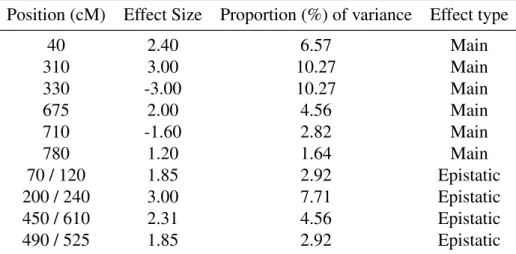
Simulation II imitates the classic QTL mapping scenario with widely spaced markers and a more complex structure of QTL genes. Forty-one markers on a single large chromosome of 800 cM were generated for 1000 backcross subjects, evenly spaced at 20 cM. Six main QTL effects and four epistatic effects were placed on the chromosome with effect sizes ranging from 1% to 10% of the total phenotypic variance. Positions of these QTL genes either overlap with a marker or lie in between markers. Details of these simulated QTL genes can be found in Table 2. We set the population mean equal to 5.0, and the error is normally distributed with mean 0 and variance 10. We replicated this simulation for 100 times.

To obtain a background marker model B_n(M), we evaluated three algorithms: Deletion Sub-stitution Addition (DSA) (Sinisi and van der Laan 2004), random forests (RF), and super learner (SL) (van der Laan et al. 2007). DSA is a search algorithm using polynomial basis functions and minimizing residual sum of squares over subsets of covariates in a regression. When restricted to main term linear models, it often produces results similar to CIM. RF is a tree-based nonparametric machine learning algorithm. In this simulation, the least aggressive fit is a linear main-term model from DSA, and we consider RF to be the most aggressive fit as it is likely to capture interaction terms. SL takes both DSA and RF as its candidate learners and finds an optimal combination of these two. Here, on average, it combines these algorithms with weights 0.59 for DSA and 0.41 for RF. See Table 3 for the average CV risk, the empirical (EM) risk, and the pMSE∗∗ risk of the B_n(M)for these three algorithms. If we had only considered the CV risk, we would have chosen SL as the bestBn(M). The differences between the CV risks for all three algorithms were subtle,

while the differences between the EM risks were more substantial. It is apparent that RF is overfit-ting because its EM risk is much smaller than its CV risk. SL takes RF as a candidate learner, and is thus also affected by this overfitting. Taking this into consideration, DSA produces the bestQ0_n. Hence, in the following analysis, we use a TMLE initialized with DSA as a reference line.

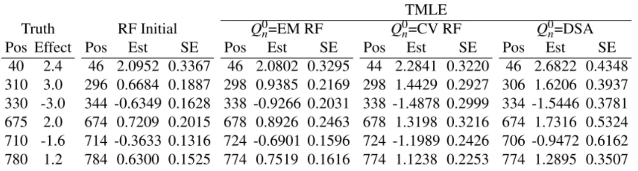
The entire chromosome was scanned with a 2-cM incremental step. In g_n(W),W₁ andW₂are the flanking markers 40 cM to A. In Table 4 and Figure 1, we report the TMLE estimates and their standard errors at genomic locations with a main QTL effect, for the RF initial estimator, TMLE(Q0_n=EM RF), TMLE(Q0_n=CV RF), and TMLE(Q0_n=DSA). (We use TMLE(Q0_n) to index TMLE with its initial estimatorQ0_n.) For RF, the initial effect estimates are far from the truth due to overfitting. When using the RF fit asQ0_n, TMLE produced better estimates than the RF initial estimator, but it was not better than TMLE(Q0_n=DSA). We then used a cross-validated RF fit asQ0_n. TMLE was able to fully recover the effect size estimates to the level of TMLE(Q0_n=DSA), while the

Table 2: True positions and effect sizes of QTL genes in Simulation II

Position (cM) Effect Size Proportion (%) of variance Effect type

40 2.40 6.57 Main 310 3.00 10.27 Main 330 -3.00 10.27 Main 675 2.00 4.56 Main 710 -1.60 2.82 Main 780 1.20 1.64 Main 70 / 120 1.85 2.92 Epistatic 200 / 240 3.00 7.71 Epistatic 450 / 610 2.31 4.56 Epistatic 490 / 525 1.85 2.92 Epistatic

Note: For epistatic effects, positions of interacting QTLs are indicated with a slash. Proportions of explained variance for epistatic effects were computed assuming interacting QTLs are independent of each other.

Table 3:The mean risk ofB_n(M)from Simulation II

SL DSA RF

EM risk 7.55(64.02%) 12.27(41.46%) 3.20(84.74%) CV risk 12.97(38.12%) 13.30(36.58%) 13.61(35.06%)

pMSE∗∗ 18.40 14.32 24.03

Table 4:The estimates of QTL main effects and their standard errors in Simulation II

TMLE

Truth RF Initial Q0_n=EM RF Q0_n=CV RF Q0_n=DSA Pos Effect Pos Est SE Pos Est SE Pos Est SE Pos Est SE

40 2.4 46 2.0952 0.3367 46 2.0802 0.3295 44 2.2841 0.3220 46 2.6822 0.4348 310 3.0 296 0.6684 0.1887 298 0.9385 0.2169 298 1.4429 0.2927 306 1.6206 0.3937 330 -3.0 344 -0.6349 0.1628 338 -0.9266 0.2031 338 -1.4878 0.2999 334 -1.5446 0.3781 675 2.0 674 0.7209 0.2015 678 0.8926 0.2463 678 1.3198 0.3216 674 1.7316 0.5324 710 -1.6 714 -0.3633 0.1316 724 -0.6901 0.1596 724 -1.1989 0.2426 706 -0.9472 0.6162 780 1.2 784 0.6300 0.1525 774 0.7519 0.1616 774 1.1238 0.2253 774 1.2895 0.3507

Positions (Pos) are in centi-morgans.

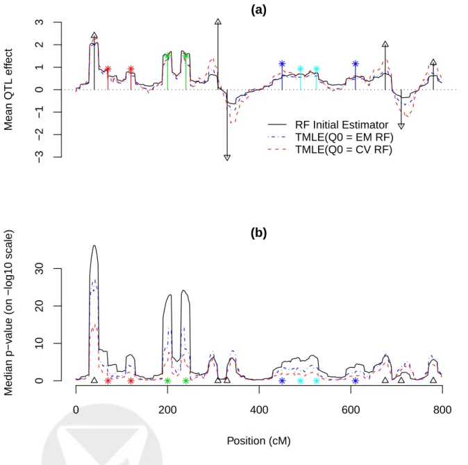
position estimates stayed essentially unchanged compared to TMLE(Q0_n=EM RF). TMLE(Q0_n=CV RF) also generated a more conservative p-value profile than TMLE(Q0_n=EM RF), as illustrated in Figure 1.

3.3

Simulation III

In Simulation III, we demonstrate the performance of C-TMLE in a simple example. We simulated 600 backcross subjects and 120 markers each spaced at 5 cM on a pseudo-chromosome. Two QTL genes were placed at marker position 110 cM and marker position 310 cM, denoted with M₍₁₁₀₎ andM₍₃₁₀₎. An epistatic effect was situated atM₍₂₀₀₎ and M₍₂₄₀₎. Error terms were drawn fromN(0,10). The two main effects atM₍₁₁₀₎ andM₍₃₁₀₎ account for 3.3% and 2.3% of the total phenotypic varaiance, respectively, and the epistatic effect accounts for 1.7% of the total variance. We generated 100 such simulation sets. Since markers were dense, our analysis did not consider positions in-between markers. Therefore, allAs are observed. The CIM output was used asQ0_n. For g_n(W)in C-TMLE, we arbitrarily excluded a 20 cM region around AfromW to avoid adjusting for strongly correlated markers.

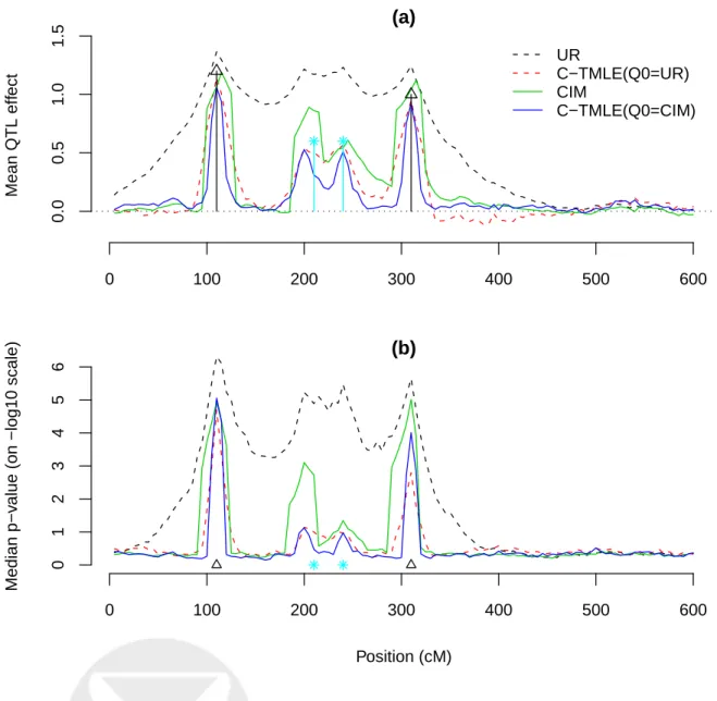
C-TMLE improved the original CIM estimates, with a better resolution and less significant p -values, as illustrated in Figure 2. We also analyzed this simulation with TMLE₍₂₀₎(see Simulation I). Compared to TMLE₍₂₀₎, C-TMLE produced similar effect estimates yet smaller standard errors, resulting in smaller p-values. As noted before, by adjusting for markers highly correlated withA ingn(W), we remove more bias in the estimate. However, additional adjustment also means larger

standard errors. In the extreme case, the model parameter β becomes unidentifiable. Thus, there

is a trade-off between using a highly predictiveg_n(W)and a conservative one, and the C-TMLE algorithm is designed to determine an optimal trade-off based on the data. In this simulation, C-TMLE selects a more conservative g_n(W) than TMLE₍₂₀₎. In general, C-TMLE is indeed less aggressive than TMLE₍₂₀₎. Choice of Q0_n also affects C-TMLE. As an illustration, we used the univariate regression (UR) fit as Q0_n. C-TMLE with the UR initial produced satisfactory results, considering the poor performance of UR. However, with the CIM initial, C-TMLE is performs even better with improved resolution and better separation of two linked interacting QTL genes (Figure 2).

−3 −2 −1 0 1 2 3 (a) Mean QTL eff ect RF Initial Estimator TMLE(Q0 = EM RF) TMLE(Q0 = CV RF) 0 200 400 600 800 0 10 20 30 (b) Position (cM) Median p−v

alue (on −log10 scale)

Figure 1: The mean effect estimate and the median p-value ofβn from simulation II. In (a), the

mean effect estimate across all simulations are plotted at each tested position, for the initial RF estimator, TMLE(Q(n0)=EM RF), and TMLE(Q(n0)=CV RF). True effect sizes and positions are

su-perimposed. Black triangles represent main QTL effects. Colored stars represent epistatic effects. Epistatic effects are halved for a clear display, and the interacting QTLs are grouped in the same color. In (b), the median p-values are plotted at each tested position in correspondence with (a).

0 100 200 300 400 500 600 0.0 0.5 1.0 1.5 (a) Mean QTL eff ect UR C−TMLE(Q0=UR) CIM C−TMLE(Q0=CIM) 0 100 200 300 400 500 600 0 1 2 3 4 5 6 (b) Position (cM) Median p−v

alue (on −log10 scale)

Figure 2: A demonstration of C-TMLE performance. In (a), the average QTL effect estimate across 100 simulations is plotted against its position, for UR, CIM, C-TMLE with UR initial, and C-TMLE with CIM initial. UR and C-TMLE with UR initial are grouped by broken lines. CIM and C-TMLE with CIM initial are grouped by solid lines. Black triangles indicate two main effects at position 110 and 310 cM. Blue stars indicate the epistatic effect at the location 200 and 240 cM, and for the ease of plotting, this epistatic effect is evenly divided betweenM₍₂₀₀₎andM₍₂₄₀₎. Dotted line is the zero line.In (b),the median p-value ofβnacross all simulations at each marker is plotted,

Table 5: The estimates of QTL effect sizes and positions from CIM and C-TMLE for the wound-healing trait

CIM C-TMLE

QTL ID Chr cM Effect size Chr cM Effect size

1 1 43.91 -0.1170 1 51.4 -0.1098 2 2 44.11 -0.0433 - - -3 2 56.41 -0.0460 2 58.3 -0.0453 4 3 28.81 -0.0531 3 32.5 -0.0487 5 4 20.61 -0.0993 4 19.4 -0.0891 6 4 55.01 -0.1024 4 57.4 -0.0979 7 6 0.01 0.0444 6 3.4 0.0478 8 6 32.21 -0.0992 6 25.4 -0.1120 9 - - - 6 33.4 -0.1148 10 6 51.91 -0.0457 6 55.4 -0.0412 11 7 30.91 0.1089 7 39.4 0.0969 12 9 43.31 -0.1582 9 46.3 -0.1714 13 - - - 11 38.5 0.05972 14 12 2.01 0.0563 12 4.3 0.05752 15 13 45.91 -0.0785 13 44.1 -0.0822 16 13 58.61 -0.0783 - - -17 - - - 17 8.1 0.05124 18 - - - 17 30.1 -0.0585

4

Data Analyses

We present three data application studies to demonstrate the utility of targeted methods in QTL data.

4.1

Wound-Healing Application

In this section, we analyze a data set published in Masinde et al. (2001). The original study was designed to identify QTL genes involved in the wound-healing process. A genomewide scan of 119 codominant markers was performed using 633 F2 (MRL/MP x SJL/J) mice. Each mouse was punctured with a 2-mm hole in its ear, and the phenotypic trait was the hole closure measurement at day 21. The marginal distribution of the phenotypic trait is bell-shaped.

We analyzed this data set with TMLE, C-TMLE, and CIM. Based on the evaluation of a dis-crete super learner (van der Laan et al. 2007) that included both DSA and random forests, the DSA machine learning algorithm was selected as initial estimator ofE₀(Y |M), and subsequently mapped into the desired initial estimator forE₀(Y |A,M−)satisfying the semiparametric regres-sion model. To lessen the computational load, we first screened additive and dominant effects of all markers with univariate regression and supplied to this machine learning algorithm the markers

0 5 10 15 20 25 Genome Location FDR adjusted p−v

alue (on −log10 scale)

1 2 3 4 5 6 7 8 9 10 11 12 13 14 15 16 17 18 19

Figure 3: The genomewide FDR adjusted p-value profile for the additive effects in the wound-healing data set. Theblack linerepresents CIM, and thered linerepresents C-TMLE. Chromosome numbers are superimposed on top of the picture.

with a p-value less than 0.10. In the TMLE, the conditional mean ofA, givenM− is fitted with a main terms linear regression model with main termsA_c,W₁a,W₁d,W₂a,W₂d, whereA_c denotes the dominant effect ofA whenA is additive and the additive effect ofAwhenAis dominant,W1and W₂are the closest flanking markers 20 cM away fromA, and the superscriptadenotes the additive effect and d the dominant effect. In C-TMLE, when A is additive,W is defined as the additive effects of all markers on the same chromosome 20 cM away fromAand the dominant effects of all markers on the same chromosome asA, and vice versa whenAis dominant.

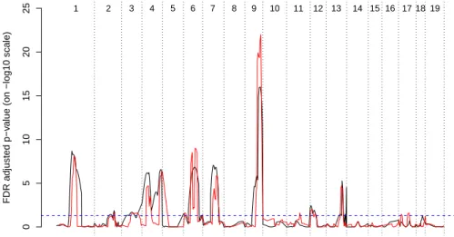
Four hundred putative QTL positions were tested at 2-cM increments for both the additive and dominant effects. The p-values were adjusted using FDR (Benjamini and Hochberg 1995). The TMLE and C-TMLE produced similar results, thus we only present C-TMLE results. Figure 3 dis-plays the genomewide FDR-adjusted p-value profile for the additive effect at each tested position. Table 5 summarizes significant QTL genes at level 0.05. The CIM p-values were computed from the asymptotic χ2 distribution. No significant dominant effect was detected in this data set. The

C-TMLE essentially identified the same QTL genes as CIM, albeit with an improved resolution. Many of these genes were also reported in Masinde et al. (2001). However, on chromosome 6, the C-TMLE suggests two linked QTL genes instead of one, as indicated by CIM.

4.2

Listeria Application

Boyartchuk et al. (2001) published a data set on the survival time of 116 age-matched female mice following infection with Listeria monocytogenes, a Gram-positive bacteria causing a wide range

Logarithm of the survival time Frequency 4.2 4.4 4.6 4.8 5.0 5.2 5.4 5.6 0 5 10 15 20 25 30 35

Figure 4: Histogram of the survival time for mice upon infection withListeria monocytogenes, on logarithm scale.

of diseases. The mice were an F2 intercross population derived from susceptible BALB/cByJ and resistant C57BL/6ByJ strains, and the goal of the study was to map genetic factors of susceptibility toL. monocytogenes. The phenotypic trait is the recorded time to death for each mouse upon in-fection withL. monocytogenes. One hundred and thirty-one codominant markers were genotyped on the autosomal chromosomes. When a mouse survived beyond 240 h, it was considered recov-ered. About 30% of the mice recovered, and we refer to them as survivors and the remaining mice as nonsurvivors. This creates a spike in the phenotypic trait distribution, violating the normality assumption in traditional approaches of QTL mapping (Figure 4).

The outcomeY was defined as the logarithm of the phenotypic trait.Y can be decomposed into a binary trait of survival or nonsurvival and a continuous trait of survival time among nonsurvivors (Broman 2003). We denote this binary trait of survival byZ=I(Y =log 264). Then, the expected value ofY given the marker dataMcan be represented as

E0(Y |M) =P0(Z=1|M)log 264+P0(Z=0|M)E0(Y |Z=0,M).

In the above formula, P₀(Z =1|M) and P₀(Z=0|M) are conditional probabilities of whether a mouse has survived (Z=1) or died (Z=0) given the marker data M. We fit this with a super

Table 6:Mean risk of candidate initial regressions in discrete super learner from the Listeria data set DSA RF SL 2-part SL CV risk 0.2212 0.1581 0.1589 0.1463 EM risk 0.0938 0.0293 0.0293 0.0246 pMSE∗∗ 0.3586 0.2868 0.2885 0.2681

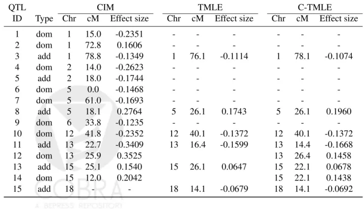
Table 7: The estimates of effect sizes and positions of QTL genes from CIM, TMLE, and

C-TMLE in the Listeria dataset. QTL genes with FDR adjusted p-values smaller than 0.05

are reported.

QTL CIM TMLE C-TMLE

ID Type Chr cM Effect size Chr cM Effect size Chr cM Effect size

1 dom 1 15.0 -0.2351 - - - -2 dom 1 72.8 0.1606 - - - -3 add 1 78.8 -0.1349 1 76.1 -0.1114 1 78.1 -0.1074 4 dom 2 14.0 -0.2623 - - - -5 add 2 18.0 -0.1744 - - - -6 dom 5 0.0 -0.1468 - - - -7 dom 5 61.0 -0.1693 - - - -8 add 5 18.1 0.2764 5 26.1 0.1743 5 26.1 0.1960 9 dom 6 33.8 -0.1235 - - - -10 dom 12 41.8 -0.2352 12 40.1 -0.1372 12 40.1 -0.1372 11 add 13 22.7 -0.3409 13 16.4 -0.1599 13 14.4 -0.1668 12 dom 13 25.9 0.3525 13 26.4 0.1458 13 add 15 25.1 0.1540 15 26.1 0.0647 15 22.1 0.0678 14 dom 15 12.0 0.2042 15 22.1 0.1438 15 add 18 - - 18 14.1 -0.0679 18 14.1 -0.0692

0 2 4 6 8 10 (a) 1 2 3 4 5 6 7 8 9 10 11 12 13 14 15 16 17 1819 0 2 4 6 8 10 (b) 1 2 3 4 5 6 7 8 9 10 11 12 13 14 15 16 17 1819 0 2 4 6 8 10 (c) 1 2 3 4 5 6 7 8 9 10 11 12 13 14 15 16 17 1819

Figure 5: The genomewide p-value profile for the additive and dominant effects in the Listeria dataset. Thep-values are FDR adjusted and on a negative log10 scale. (a) thep-value profile from the CIM. (b) p-value profile from the TMLE. (c) p-value profile from the C-TMLE. In all three panels, theblack solid linerepresents additive effects, and theblue dashed linerepresents dominant effect. The black dash-dot line indicates the 0.05 p-value threshold. Chromosome numbers are superimposed on top of each panel.

learning algorithm for binary outcomes. E₀(Y |Z=0,M)is the conditional expectation ofY onM given that the mouse has died, which can be obtained by applying super learning on nonsurvivors. We refer to this machine learning algorithm as the 2-part super learner.

The collection of algorithms in the super learner included DSA and random forests. As before, the machine learning algorithms were only provided the additive and dominant markers that had a significant univariate effect based on a p-value threshold of 0.10. Since we wished to evaluate if this 2-part super learner provided a better fit than a regular super learner, we implemented a discrete super learner whose library consisted of a total of four algorithms for estimation of E0(Y |M):

DSA, random forests, super learner, and a 2-part super learner. In Table 6, we report the EM risk, the CV risk, and the pMSE∗∗ of DSA, RF, SL, and the 2-part SL. In the super learning fits, more than 95% of the weight was put on random forests, thereby strongly favoring a fit that allows for complex interactions.

The 2-part super learner had the smallest risk for all three types of risk and was therefore selected as the estimator ofE0(Y |M). In the TMLE, we fitted the conditional mean of A, given M−, with a main term linear regression model including the main terms usedA_c,W₁a,W₁d,W₂a,W₂d,

whereA_cdenotes the dominant effect ofAwhenAis additive and the additive effect ofAwhenA is dominant,W1andW2are the closest flanking markers 20 cM away fromA, and the superscripta

denotes the additive effect andd the dominant effect.

When inspecting Fig. 5, TMLE and C-TMLE display much less noise than the parametric CIM. Three additive genes on chromosomes 1, 5, and 13 are clearly identified. Two additive effects on chromosomes 15 and 18 are borderline significant. In addition, C-TMLE also detected dominant effects on chromosomes 12, 13, and 15. The chromosome 15 QTL gene is identified as carrying both the additive and dominant effects. The literature suggests that the chromosome 1 QTL gene has an effect on how long a mouse can live given it will eventually die, the chromosome 5 gene has an effect on a mouse’s chance of survival, and the genes on chromosomes 13 and 15 are involved in both (Boyartchuk et al. 2001; Broman 2003; Jin et al. 2007). We detected all of these genes and, in addition, an additive gene on chromosome 18 and a dominant gene on chromosome 12. CIM also identified those major genes, however, with less significance and many more suspicious positives. See Table 7.

4.3

Yeast Data Set

In this section, we analyze an expression QTL dataset. The original data came from Brem et al. (2002), consisting of 6216 expression traits and 3312 markers on 112 haploid segregates of budding yeast. Genotypes of markers are dichotomous, and many markers have identical genotypes. We dropped all the redundant markers, resulting in 972 markers. Missing markers were imputed based on the linkage disequilibrium (LD) information of the nearby regions. A fast version of TMLE was applied to this dataset. The initial estimatorQ0_nis from univariate regression (UR), andg_n(W) is a linear regression with covariatesW1 andW2, whereW1 andW2 are markers on both sides of A with LD R2=0.2 to A. This strategy essentially consists of three simple linear regressions: Y ∼A, A∼W₁+W₂, and theε-regression. In this special case, the TMLE estimate forβ will be

equivalent to the coefficient ofAfrom the multiple regressionY ∼A+W1+W2, which means that

our semiparametric model is reduced to a simple parametric model. Since we are using a simple Q0_nthat is unlikely to capture the truth, the consistency ofβnnow relies largely on the fit ofgn(W).

Table 8: Significant QTL hotspots detected by the UR and the TMLE in the yeast dataset. Significant QTL hotspots are defined as the QTL linked to more than 26 gene expression traits for the UR, and 20 traits for the TMLE. Column “n” is the number of genes linked to the QTL hotspot

Univariate Regression TMLE

chr start end n cis-linked genes chr start end n cis-linked genes 1 40 60 32 OAF1, YAL049C, YAL046C 1 40 60 25 SAME

1 180 200 21 YAR028W, UIP3, MST28 2 300 320 75 N/A 2 360 380 142 ECM2, TRM7, NRG2, YBR064W, TIP1, TAT1 2 360 380 21 SAME 2 500 580 593 CNS1, TBS1, CSH1, DEM1, PEX32, TOS1, TYR1, NPL4, YBR137W

2 500 580 333 SAME 2 640 680 86 N/A

3 60 100 279 LEU2, RNQ1, FRM2 3 60 100 201 SAME

3 100 120 65 N/A 3 100 120 50 N/A

3 200 220 67 YCR041W, MATALPHA2, MATAL-PHA1, TAF2, RSC6

3 200 220 50 SAME

4 920 940 111 N/A 4 920 940 73 N/A

4 1140 1160 29 YDR339C 4 1520 1540 28 YDR544C, YRF1-1 4 1520 1540 27 SAME

5 100 120 49 URA3, GEA2 5 100 120 41 URA3

5 340 360 148 N/A 5 340 360 23 N/A

5 380 400 72 N/A 5 380 400 23 N/A

5 420 440 155 N/A 5 420 440 32 N/A

7 40 60 135 TAD1 7 40 60 29 SAME

8 80 120 151 GPA1, YAP3, YHL010C, SHU1 8 80 120 90 SAME

9 20 40 44 YIL169C, YIL166C, YIL163C 10 20 40 36 YJL213W, YJL218W, YJL217W 10 20 40 22 YJL218W, YJL217W 10 80 100 30 SWI3, ATG27, CPS1

12 500 520 36 YLR173W, DPH5, IDP2, YLR179C, RFX1

12 500 520 32 SAME

12 640 720 256 HAP1, NEJ1, YLR283W, YLR287C 12 640 660 121 HAP1 12 880 900 27 N/A

12 940 960 27 YLR414C

12 1040 1060 55 YLR455W 12 1040 1080 84 YLR455W, YLR462W, YLR464W, YLR463C

13 40 60 109 N/A 13 40 60 123 N/A

13 540 560 39 N/A 14 440 460 413 YPT53, RHO2, YNL089C, TOP2 14 440 460 330 SAME

14 480 500 222 LAT1, MSK1 14 480 540 162 LAT1, MSK1, AQR1 14 540 560 39 SLM2, YNL046W, YNL040W

15 140 200 517 HMI1, SPO21, RFC4, YOL092W, HAL9, YOL085C, ATG19, PHM7

15 140 180 405 SAME 15 280 300 28 YOL019W, YOL014W 15 280 300 22 SAME

15 560 580 62 YOR131C 15 560 580 56 SAME

16 420 440 41 CWC27

Despite the simplicity of this approach, there were substantial improvements in TMLE compared to UR (Figure 6), and one can use this fast TMLE as a more reliable screening tool.

We surveyed all the gene-marker pairs with TMLE and UR.P-values were adjusted with FDR, pooling all the tests. The 0.05 FDR cutoff for UR was 0.00028, and for TMLE was 0.00011. Redundant linkages were handled as in Wang et al. (2006), where at most one QTL is assumed on each chromosome. In Table 9, we report the number of gene expression traits with multiple QTL at an FDR 0.05 level for both UR and TMLE. With UR, there are 2997 gene expression traits detected with more than 2 QTL, while with TMLE, this number is reduced to 1837. In Zou and Zeng (2009), 1242 traits are claimed to have multiple QTL with a sequential multiple interval mapping procedure. We also summarized our results in terms of the QTL hotspots — small genomic regions linked to multiple gene expression profiles. The yeast genome was divided into 611 20-Kb bins, and the number of non-redundant linkages to each bin were counted. For UR, there are 6430 linkages to 752 markers; for TMLE, there are 4304 linkages to 702 markers.

0 200 400 600 0 5 10 15 Gene BTS1 Kb −log10 p−v alue UR TMLE

Figure 6: An individual example of how the TMLE achieves a better resolution than the UR for a QTL on chromosome 2 for gene expression trait BTS1. They-axis is the negative log10 p-value, thex-axis represents the chromosome 2 in Kb. Black line represents the UR, and red line represents the TMLE.

Table 9: The number of genes tabulated with the number of QTL linked to the gene for the yeast data set

Number of QTL 0 1 2 3 4 5 6 7

UR 1127 2051 1726 895 297 65 13 1

TMLE 2042 2296 1249 460 108 16 4 0

We also assessed cis-linked genes at significant QTL hotspots and listed these genes in Table 8. A cis-gene is defined as an expression trait gene with a QTL linked to itself within a 10 Kb upstream and downstream window. Our results are essentially consistent with what has been reported in the literature (Brem et al. 2002; Sun et al. 2007).

5

Discussion

Current practice for assessing the effects of genes on a phenotype involves the utilization of para-metric regression models. One of the advantages of parapara-metric regression models is that they also provide a p-value, allowing one to rank the different estimated effects and assess their significance. However, both the effect estimates as well as the reported statistical significance are subject to bias due to model misspecification. On the other hand, machine learning algorithms such as random forest, are not sufficient when used alone since these algorithms are tailored for prediction, report generally poor effect estimates, and do not provide a measure of significance. C-TMLE allows us to incorporate the state of the art in machine learning, without significant computational burden (the targeting step is relatively trivial, although it needs to be carried out for each effect), while still providing an estimate tailored for the effect of interest and CLT-based statistical inference.

References

C.J. Basten, B.S. Weir, and Z.B. Zeng. QTL Cartographer, 2001. URL

http://statgen.ncsu.edu/qtlcart/.

Y. Benjamini and Y. Hochberg. Controlling the false discovery rate: a practical and powerful approach to multiple testing. J R Stat Soc Ser B, 57:289–300, 1995.

V.L. Boyartchuk, K.W. Broman, R.E. Mosher, S.E.F. D’Orazio, M.N. Starnbach, and W.F. Dietrich. Multigenic control of listeria monocytogenes susceptibility in mice. Nat Genet, 2001.

L. Breiman. Random forests. Mach Learn, 45:5–32, 2001.

R.B. Brem, G. Yvert, R. Clinton, and L. Kruglyak. Genetic dissection of transcriptional regulation in budding yeast. Science, 296:752–755, 2002.

K.W. Broman. Mapping quantitative trait loci in the case of a spike in the phenotype distribution. Genetics, 2003.

C.S. Haley and S.A. Knott. A simple regression method for mapping quantitative trait loci in line crosses using flanking markers. Heredity, 1992.

S.C. Heath. Markov chain Monte Carlo segregation and linkage analysis of oligogenic models. Am J Hum Genet, 1997.

R.C. Jansen. Interval mapping of multiple quantitative trait loci. Genetics, 1993.

C. Jin, J.P. Fine, and B.S. Yandell. A unified semiparametric framework for quantitative trait loci analysis, with application to spike phenotypes. J Am Stat Assoc, 2007.

C.H. Kao, Z.B. Zeng, and R.D. Teasdale. Multiple interval mapping for quantitative trait loci. Genetics, 1999.

E.S. Lander and D. Botstein. Mapping Mendelian factors underlying quantitative traits using RFLP linkage maps. Genetics, 1989.

S.S.F. Lee, L. Sun, R. Kustra, and S.B. Bull. EM-random forest and new measures of variable importance for multi-locus quantitative trait linkage analysis. Bioinformatics, 2008.

G.L. Masinde, X. Li, W. Gu, H. Davidson, S. Mohan, and D.J. Baylink. Identification of wound healing/regeneration quantitative trait loci (QTL) at multiple time points that explain seventy percent of variance in (MRL/MpJ and SJL/J) mice F2 population. Genome Res, 2001.

J.M. Satagopan, B.S. Yandell, M.A. Newton, and T.C. Osborn. A Bayesian approach to detect quantitative trait loci using Markov chain Monte Carlo. Genetics, 1996.

K. Sax. The association of size difference with seed-coat pattern and pigmentation inPhaseolus vulgaris. Genetics, 1923.

M.J. Sillanpaa and E. Arjas. Bayesian mapping of multiple quantitative trait loci from incomplete inbred line cross data. Genetics, 1998.

S.E. Sinisi and M.J. van der Laan. Deletion/Substitution/Addition algorithm in learning with ap-plications in genomics. Stat Appl Genet Mol, 3(1), 2004. Article 18.

W. Sun, T. Yu, and K.C. Li. Detection of eqtl modules mediated by activity levels of transcription factors. Bioinformatics, 23:2290–2297, 2007.

J.M. Thoday. Location of polygenes. Nature, 1960.

C. Tuglus and M.J. van der Laan. Targeted methods for biomarker discovery. In M.J. van der Laan and S. Rose, Targeted Learning: Causal Inference for Observational and Experimental Data. Springer, Berlin Heidelberg New York, 2011.

M.J. van der Laan and S. Gruber. Collaborative double robust penalized targeted maximum likeli-hood estimation. Int J Biostat, 6(1):Article 17, 2010.

M.J. van der Laan and J.M. Robins.Unified Methods for Censored Longitudinal Data and Causal-ity. Springer, Berlin Heidelberg New York, 2003.

M.J. van der Laan and S. Rose. Targeted Learning: Causal Inference for Observational and Experimental Data. Springer, Berlin Heidelberg New York, 2011.

M.J. van der Laan and Daniel B. Rubin. Targeted maximum likelihood learning. Int J Biostat, 2 (1):Article 11, 2006.

M.J. van der Laan, E.C. Polley, and A.E. Hubbard. Super learner. Stat Appl Genet Mol, 6(1): Article 25, 2007.

H. Wang, S. Rose, and M.J. van der Laan. Finding quantitative trait loci genes with collabo-rative targeted maximum likelihood learning. Stat Prob Lett, published online 11 Nov (doi: 10.1016/j.spl.2010.11.001), 2010.

H. Wang, S. Rose, and M.J. van der Laan. Finding quantitative trait loci genes. In M.J. van der Laan and S. Rose, Targeted Learning: Causal Inference for Observational and Experimental Data. Springer, Berlin Heidelberg New York, 2011.

S. Wang, M Yehya, E.E. Schadt, H. Wang, T.A. Drake, and A.J. Lusis. Genetic and genomic analysis of a fat mass trait with complex inheritance reveals marked sex specificity.PLoS Genet, 2:e15, 2006.

Z.B. Zeng. Precision mapping of quantitative trait loci. Genetics, 1994.

W. Zou and Z.B. Zeng. Multiple interval mapping for gene expression qtl analysis. Genetica, 137: 125–134, 2009.