FINANCIAL TIME SERIES PREDICTION USING MACHINE
LEARNING ALGORITHMS
by
LESLIE TIONG CHING OW
Submitted in total fulfilment of the requirements
for the
MSc in Computer Science (By Research)
at Sunway University
August 2012
Copyright © 2013 by Sunway University
All rights reserved.
i | P a g e
LIST OF PUBLICATIONS
- Tiong, L.C.O., Ngo D.C.L. & Lee, Y. (2012), “Stock Price Prediction Model using Candlestick Pattern Feature.” in International Conference of Interactive Digital Media (pp. 394-401), Langkawi. [Published]
- Tiong, L.C.O., Ngo D.C.L. & Lee, Y. (2013), "Forex Trading Prediction using Linear Regression Line, Artificial Neural Network and Dynamic Time Warping Algorithms." in Proceedings of the 4th International Conference on Computing and Informatics (pp. 71 – 77), Kuching Sarawak. [Published]
ii | P a g e
ACKNOWLEDGMENT
First of all, I would like to express my gratitude to my supervisors Dr Lee Yun Li and Professor David Ngo Chek Ling for the useful comments, remarks and engagement through the learning process of this research. Furthermore, I would like to thank Mr. Edric Yap Eu Soon, Mr. Kho Ing Chao and Mr. Tan Yong An for providing the information and knowledge of financial time series as well for the support. I would also like to thank Mr. Akputu Kingsley, Mr. Lim Kai Li, Ms Loo Tze Jin and Mr. Mansoor Ebrahim, for their encouragement and insightful comments. Without the particular assists that mentioned above, I would face many difficulties while doing this.
iii | P a g e
ABSTRACT
Financial time series prediction is a challenging task due to the fluctuation of trading or economic exchange that is difficult to predict. Researchers from different fields have been attracted to perform several techniques for identifying reliability of the financial time series prediction. Finding of research papers, the financial trend patterns repeat itself in the history. Thus, this research motivates and aims to investigate the repeat behaviour and pattern of trends from the historical financial time series data, and utilise the strength of machine learning techniques to develop a promising financial time series predictor engine. In this research, two frameworks are proposed for financial time series prediction. In the first proposed framework, candlestick pattern is utilised as technical analysis method to identify the financial trends. Thereafter, Artificial Neural Network (ANN) and Support Vector Machine (SVM) algorithms are implemented separately to train with the trend patterns for predicting the movement direction of financial trends. In the second proposed framework, Linear Regression Line (LRL) is utilised to identify the trend patterns from historical financial time series, which is supported by ANN and SVM for classification process separately. Subsequently, Dynamic Time Warping (DTW) algorithm is utilised through brute force to predict the trend movement. The experimental results showed that the second proposed model is consistent with the hypothesis, which provides better accuracy of prediction. Therefore, the findings of this research help in improving the accuracy of prediction model.
iv | P a g e
TABLE OF CONTENTS
1.0 INTRODUCTION ... 1
1.1 Overview of Financial Market ... 1
1.2 Concept of Financial Time Series ... 2
1.3 The Financial Time Series Prediction ... 4
1.4 Scope ... 8
1.5 Problem Statements ... 9
1.6 Aim and Objectives ... 10
1.7 Contributions ... 12
1.8 Thesis Layout ... 13
2.0 LITERATURE REVIEW ... 14
2.1 Feature Extraction of Financial Time Series... 14
2.1.1 Financial Time Series: Stock Chart ... 15
2.1.2 Financial Time Series: Technical Indicators ... 24
2.2 Prediction Techniques – Artificial Intelligence (AI) Techniques ... 34
2.2.1 Expert System (ES) ... 35
2.2.2 Machine Learning Algorithms ... 39
v | P a g e
2.3 Dynamic Time Warping (DTW) Algorithm ... 57
2.4 Review Summary ... 60
3.0 PROPOSED FRAMEWORK ... 62
3.1 Candlestick Chart and Machine Learning Algorithms ... 63
3.1.1 Candlestick Pattern as Pattern Analysis method ... 64
3.1.2 Learning Process and Evaluation using Machine Learning Algorithms70 3.2 LRL, K-Mean and Machine Learning Algorithms ... 73
3.2.1 Pattern Analysis method ... 73
3.2.2 Classification Process of Machine Learning Algorithms ... 82
3.2.3 DTW Prediction ... 84
4.0 EXPERIMENTAL RESULT AND DISCUSSION ... 89
4.1 Candlestick Pattern and Machine Learning Algorithms ... 89
4.1.1 Pattern Analysis ... 89
4.1.2 Classification ... 97
4.2 LRL, K-Mean and Machine Learning Algorithms ... 101
4.2.1 Pattern Analysis ... 101
vi | P a g e
4.2.3 Prediction ... 109
4.3 Experiment Summary ... 117
5.0 CONCLUSION AND FUTURE WORK ... 118
5.1 Conclusion ... 118
5.2 Future Work ... 119
REFERENCES ... 121
APPENDIX ... 129
Screen Shot – Preliminary Prediction Model ... 129
Screen Shot – Proposed Prediction Model ... 131
LIST OF FIGURES Figure 1.1 - Example of Financial Time Series Data for Forex Trading ... 3
Figure 1.2 - Structure of Second Proposed Framework... 7
Figure 2.1 - Example of Stock Chart ... 16
Figure 2.2 - Structure of Candlestick Pattern ... 17
Figure 2.3 - Structure of OHLC Bar Chart ... 21
Figure 2.4 - Concept of Trend Position ... 22
vii | P a g e
Figure 2.6 - MACD Indicator ... 31
Figure 2.7 - Stochastic Oscillator ... 33
Figure 2.8 - Basic Structure of an ES ... 36
Figure 2.9 - The Concept and Structure of ANN algorithm ... 40
Figure 2.10 - Structure of HMM ... 46
Figure 2.11 - Structure of SVM with a Kernel Function ... 50
Figure 2.12 - A warping path between two time series data ... 58
Figure 3.1 - General Ideas of Proposed Frameworks ... 62
Figure 3.2 - The Proposed Framework of Financial Time Series Analysis using Candlestick Chart ... 64
Figure 3.3 - Rules for identifying the Colour of RB ... 66
Figure 3.4 - Rules for Identifying the Position of Candlestick Pattern ... 67
Figure 3.5 - Candlestick Representation Algorithm... 69
Figure 3.6 - The Learning and Evaluation Processes of the Prediction Model ... 70
Figure 3.7 - Learning Process with Candlestick Pattern Algorithm ... 72
Figure 3.8 - Classification of Candlestick Pattern Algorithm ... 72
Figure 3.9 - The Proposed Framework of Financial Time Series Analysis using LRL ... 74
viii | P a g e
Figure 3.10 - Implementation of Equation 2.2... 75
Figure 3.11 - Different Types of Trend Patterns ... 76
Figure 3.12 - Proposed Features ... 76
Figure 3.13 - Pattern Segmentation Algorithm ... 78
Figure 3.14 - Illustration of Proposed Features ... 79
Figure 3.15 - Features Creation Algorithm ... 81
Figure 3.16 - K-mean Algorithm ... 81
Figure 3.17 - Classification Process of Machine Learning Algorithms ... 82
Figure 3.18 - Learning Process with Selected Features Algorithm ... 83
Figure 3.19 - Classification of Trend Patterns Algorithm ... 84
Figure 3.20 - Implementation of DTW for Prediction ... 85
Figure 3.21 - Optimising the Shortest Warping Path using DTW ... 86
Figure 3.22 - 2 × 2 Structure Elements Algorithm ... 87
Figure 3.23 - Basic Idea for Identifying the Diagonal Direction ... 87
Figure 3.24 - The Steps of Using 2 × 2 Structure Elements to Identify the Diagonal Direction ... 88
Figure 4.1 - Financial Time Series Data AUD – USD in January 2011 ... 90
ix | P a g e
Figure 4.3 - Large Down Position ... 95
Figure 4.4 - Small Up Position ... 95
Figure 4.5 - Small Down Position ... 95
Figure 4.6 - Small Inside Position ... 95
Figure 4.7 - Small Outside Position ... 95
Figure 4.8 - Large Inside Position ... 96
Figure 4.9 - Large Outside Position ... 96
Figure 4.10 - Financial Trend in Histogram Chart: AUD – USD 2nd Week in January 2011 ... 102
Figure 4.11 - Financial Trend in Histogram Chart: AUD – USD 4nd Week in April 2011 ... 102
Figure 4.12 - Financial Trend in Histogram Chart: EUR – USD 3nd Week in July 2011... 103
Figure 4.13 - Financial Trend in Histogram Chart: EUR – USD 4nd Week in September 2011 ... 103
Figure 4.14 - Downtrend Sample 1 ... 104
Figure 4.15 - Downtrend Sample 2 ... 104
Figure 4.16 - Downtrend Sample 3 ... 105
x | P a g e
Figure 4.18 - Uptrend Sample 2... 105
Figure 4.19 - Uptrend Sample 3... 105
Figure 4.20 - Concept of Selected Features ... 106
Figure 4.21 - Partial Unknown Pattern ... 109
Figure 4.22 - Full Train Pattern ... 109
Figure 4.23 - Demonstration in Tracing Minimum Value ... 110
Figure 4.24 - Shortest Warping Path ... 112
Figure 4.25 - Sample 1 Prediction Result for AUD – USD in 2012 ... 113
Figure 4.26 - Sample 2 Prediction Result for AUD – USD in 2012 ... 113
Figure 4.27 - Sample 3 Prediction Result for AUD – USD in 2012 ... 114
Figure 4.28 - Sample 4 Prediction Result for EUR – USD in 2012 ... 114
Figure 4.29 - Sample 5 Prediction Result for EUR – USD in 2012 ... 115
Appendix 1 - The Learning Process of ANN using Candlestick Pattern as Features ... 129
Appendix 2 - The Learning Process of SVM using Candlestick Pattern as Features ... 130
Appendix 3 - Clustering Result using K – mean Algorithm ... 131
xi | P a g e
Appendix 5 - Prediction Result ... 133
LIST OF TABLES Table 2.1 - Review of Financial Time Series Prediction Model using Candlestick Pattern ... 19
Table 2.2 - Review of Financial Time Series Prediction Model using OHLC Bar Chart ... 23
Table 2.3 - Review of Financial Time Series Prediction Model using EMA ... 26
Table 2.4 - Review of Financial Time Series Prediction Model using LRL ... 29
Table 2.5 - Review of Financial Time Series Prediction Model using MACD ... 32
Table 2.6 - Review of Financial Time Series Prediction Model using ES ... 38
Table 2.7 - Review of Financial Time Series Prediction Model using ANN ... 43
Table 2.8 - Review of Financial Time Series Prediction Model using HMM ... 49
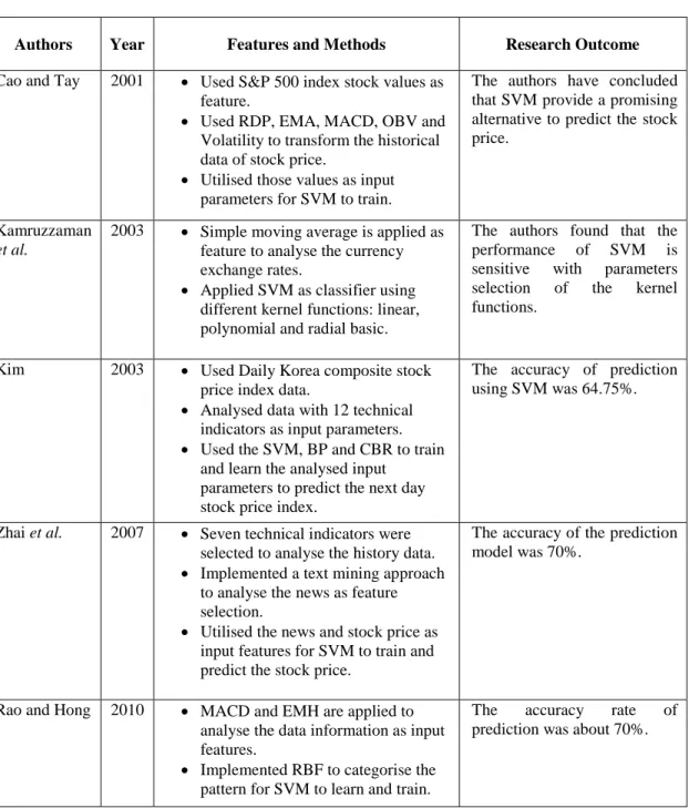
Table 2.9 - Review of Financial Time Series Prediction Model using SVM ... 53
Table 2.10 - Review of Financial Time Series Prediction Models using Hybrid Intelligence Systems ... 56
Table 3.1 - Attributes of Financial Time Series Data ... 65
xii | P a g e
Table 3.3 - Proposed Features... 78
Table 3.4 - Selected Features Representation ... 83
Table 4.1 - Sample Result of Candlestick Chart in Numeric Format ... 93
Table 4.2 - Sample Results of Second Case ... 96
Table 4.3 - First Case Candlestick Patterns as Input Parameters... 98
Table 4.4 - Second Case Candlestick Patterns as Input Parameters ... 99
Table 4.5 - Evaluation Result using Candlestick Patterns as Features for First Case ... 99
Table 4.6 - Evaluation Result using Candlestick Patterns as Features for Second Case ... 100
Table 4.7 - Sample of Clustering Result using Proposed Features ... 106
Table 4.8 - Proposed Features as Input Parameters ... 108
Table 4.9 - Using Proposed Features as Input Features for Classification ... 109
Table 4.10 - Cost Matrix Table ... 111
Table 4.11 - Confusion Matrix Table for Future Trend Prediction Result of 40 cases using AUD – USD data in 2012 ... 116
Table 4.12 - Confusion Matrix Table for Future Trend Prediction Result of 40 cases using EUR – USD data in 2012 ... 116
xiii | P a g e
LIST OF ABBREVIATIONS
AI Artificial Intelligence
ANN Artificial Neural Network
AUD Australian Dollar
CBR Case – Based Reasoning
DTW Dynamic Time Warping
EMA Exponential Moving Average
ES Expert System
EUR European Union Dollar
FL Fuzzy Logic
Forex Foreign Exchange Market
HMM Hidden Markov Model
ID3 Iterative Dichotomiser 3
LRL Linear Regression Line
LS Lower Shadow of Candlestick Chart
MACD Moving Average Convergence-Divergence
MAE Mean Absolute Error
MAP Maximum a Posteriori
MLP Multi-Layer Perceptron
OHLC Open, High, Low, Close
RB Real Body of Candlestick Chart
RBF Radial Basic Function
RMSE Root Mean Square Error
RTC Regression Trend Channel
SMO Sequential Minimal Optimisation
SOM Self – Organising Map
SVM Support Vector Machine
US Upper Shadow of Candlestick Chart
1 | P a g e
1.0 INTRODUCTION
This chapter describes the basic concepts of financial time series, issues related to prediction accuracy and the limitations of technical analysis methods. In addition, researchers from the fields of finance and computer science have implemented different types of techniques such as technical analysis methods and Artificial Intelligence (AI) to analyse the financial trends for predictions. The pros and cons of the techniques are discussed in this chapter. Furthermore, motivation and objective of developing a prediction model using machine learning algorithms are also presented.
1.1 Overview of Financial Market
Generally, financial market is defined as a marketplace where the process of economic exchange or trade is carried out between buyers and sellers, such as Foreign Exchange (Forex), stock exchange markets and others. The process involves the transfer of funds and financial assets between two or more parties (Ching, 2009). Within the financial field, financial markets are commonly referred to as markets, which are used for finance operations, expansion and economic growth (Vinci & Darskuviene, 2010).
The financial market plays an important role in promoting economic growth. The collection and analysis of financial time series data, as well as investment opportunities are provided to investors, brokers, corporations and other financial institutions. The collection of information assists them in directing funds for the most effective returns
2 | P a g e (Jalloh, 2009). The structure of financial market allows buyers and sellers to determine the price and value of financial claims or the desired rate of return on different types of financial assets. Furthermore, the financial market offers liquidity for investors through the ability to convert financial assets into liquid funds.
1.2 Concept of Financial Time Series
In financial market, financial time series data is defined as a sequence of repeated observation variables, such as stock price, currency exchange rates, bonds return and commodities price which measures at uniform time intervals. Financial time series data can be described as:
{ } (1.1)
is defined as a dataset of time series, until are defined as a sequential of different variables in different time stamp intervals. The entire variable values of are treated randomly as they are dependent on the trading and investment.
The basic variables of financial time series data include time stamp, open price, high price, low price, close price and the number of volumes bought. Those variables are described as:
3 | P a g e where i is defined as time stamp, is defined as a single data record in financial time series, is defined as opening price of the current time stamp, is defined as highest price of the current time stamp, is defined as lowest price of current time stamp, is defined as closing price of the current time stamp, and is defined as the volume.
Figure 1.1 shows an example of Forex trading that involves the currency exchange rates between EUR – USD on 2nd January of 2011 from 17:00 to 23:59. As can be seen, the financial time series data is a sequence of non-stationary values at regular intervals over different time stamp.
Figure 1.1 - Example of Financial Time Series Data for Forex Trading 1.266 1.267 1.268 1.269 1.27 1.271 17 :0 0 17 :1 7 17 :3 4 17 :5 1 18 :0 8 18 :2 5 18 :4 2 18 :5 9 19 :1 6 19 :3 3 19 :5 0 20 :0 7 20 :2 4 20 :4 1 20 :5 8 21 :1 5 21 :3 2 21 :4 9 22 :06 22 :2 3 22 :4 0 22 :5 7 23 :1 4 23 :3 1 23 :4 8
4 | P a g e
1.3 The Financial Time Series Prediction
Financial time series data is non-stationary, as it is influenced by the variations in supply and demand of investors. It is affected by many correlated factors including economic, political and even psychological ones. The reason is that financial market facilitates exchange between buyers and sellers, and reduces unsecure issues from investment. The operation of financial market has been measured as very important task in global economy field. Therefore, any fluctuation in financial market will affect the market cap of corporation and the economic growth of industries and countries.
There are some risks when investing in financial market due to the uncertainty in movement of financial time series. Investing in financial market that has no prediction and accuracy information for market performance may expose an investor to both high risk of market prediction and improper time estimation for entrance. To avoid these issues, most investors prefer to have a tool with intelligence techniques in order to minimise investment risk so that they would have higher chances in gaining profit from the investment.
Financial time series prediction relates the current economic growth of a society to future business conditions. Prediction concerns likely factors that may affect a prospective business. It also identifies the trends in order to provide decision making about the future prospect of the financial investment. However, financial time series prediction is a non-linear dynamic field due to the non-stationary and noise of time series data as the major challenges. This is because the financial market is affected by
5 | P a g e both external and internal trading. This also concerns the valuation of assets, and speculation about future events. Traditionally, the time series data obtained does not contain sufficient information to understand the future trends. Therefore, the level of difficulty in predicting the financial time series data is high.
Since 1970s, there are a large amount of intensive researches have been discovered for financial time series prediction. Researchers from the fields of finance and computer science have carried out several techniques in order to accomplish one goal, which is predicting the trend movement to yield profit. In the early stage of the financial field, technical analysis methods such as Exponential Moving Average (EMA), candlestick pattern, OHLC (Open, High, Low and Close) bar chart, stochastic oscillator, Linear Regression Line (LRL) and Moving Average Convergence-Divergence (MACD) have been proposed and implemented by researchers to investigate the financial trends for developing the prediction model (Exponential Moving Average, 2012; Linear Regression Slope Indicator, n.d.; Using Technical Indicators, 2009; Kuepper, 2012). These methods are implemented to assist the investors in identifying the trend patterns based on historical time series data. However, these methods are not reliable; this could be due to lack of ability to learn the patterns and behaviour of time series data.
Due to the rapid growth of computational intelligence, computer science researchers have involved and applied certain Artificial Intelligence (AI) techniques such as Artificial Neural Network (ANN), Fuzzy Logic (FL), Expert Systems (ES), Hidden Markov Model (HMM) and Support Vector Machine (SVM) with the technical analysis
6 | P a g e methods to predict the movement of financial trend (Cao & Tay, 2001; Charkha, 2008; Enke, Grauer, & Mehdiyev, 2011; Hassan, Nath, & Kirley, 2007; K. H. Lee & Jo, 1999). There are certain trading tools, prediction software and investment management platforms in the industry that can handle information and signals of the financial markets, such as TradeStation, MetaStock and MetaTrader (MetaStock, 1982; MetaTrader, 2000; TradeStation, 2001). These tools utilise AI techniques and technical analysis methods to provide more reliable decision-making for investors. The researchers proved that the combination of AI techniques and technical analysis methods could be a promising approach in identifying the patterns and behaviour of financial trend.
Despite the existence of trading tools and software, as well as the experiments done by past researchers, financial time series prediction models are still a very active topic for development and improvement. Thus, this thesis introduces a proposed framework using LRL for pattern analysis, supported by ANN or SVM as classifiers, and then utilises Dynamic Time Warping (DTW) algorithm to predict the following day of trends.
In the first proposed prediction framework, the candlestick pattern is applied to represent the behaviour and pattern of historical financial time series data. The candlestick pattern is formalised in terms of numeric and nominal values using equations and trading rules. Formalisation is used to represent the candlestick pattern as an input parameter for AI techniques to learn the patterns during learning process. Subsequently, ANN and SVM are implemented as classifiers to predict the movement direction of financial trends based on the selected features. From the preliminary results of this
7 | P a g e framework, the candlestick pattern is not considered as good features for representing the trend patterns.
To represent the trend patterns in a more reliable way, the implementation of LRL has been utilised for analysing and forming the overall trend patterns based on the historical financial time series data in the second proposed prediction framework. Figure 1.2 illustrates the concept of this framework. The proposed features that consist of starting point, ending point, minimum area and the sequential series of trend are utilised for identifying and segmenting the trend patterns. After the segmentation, clustering algorithm – K-mean (Kanungo et al., 2002) is implemented to cluster the trend patterns into two main classes – “Uptrend” and “Downtrend”.
Sequentially, ANN and SVM are implemented separately as classifiers to learn the trend patterns that are analysed by LRL. The selected features representation of trend patterns that are extracted from “Uptrend” and “Downtrend” are then used in the training process of ANN and SVM. Before the training process of ANN and SVM on the trend
Pattern Analysis Feature Extraction Clustering Training and Classification Prediction Feature Representation
8 | P a g e patterns, feature selection plays an important role as both machine learning algorithms could not be well-trained without reliable feature representation.
To predict future trends of the financial market, DTW is used to measure the similarity of testing trend patterns and training trend patterns in the proposed prediction model. Once the tested trend patterns have been classified as one of the trained group, DTW is applied in order to compare the tested trend patterns through brute force against the training trend patterns from the database to identify the shortest warping path.
1.4 Scope
In this thesis, the US Dollar (USD) and other major currencies, particularly the Australian Dollar (AUD) and European Union Dollar (EUR) are selected as the historical financial time series data, which consists of half-hour closing prices. Based on the historical financial time series data mentioned, LRL is applied to analyse the trend patterns, supported by ANN and SVM as classifiers separately. Then, DTW is implemented to predict the direction of future trends in the financial market.
9 | P a g e
1.5 Problem Statements
Financial time series prediction is a very complex and non-dynamic field that has been characterised by unstructured environment, uncertain motion of financial time series, hidden, noise or non-stationary raw data. There are many factors that influence the process of financial market, such as general economic conditions, supply and demand of the investment. As a result of these factors and effects, the accuracy of financial time series prediction has attracted most research interest in identifying reliability of existing frameworks for financial time series prediction.
Most researchers do not fully utilise the behaviour and patterns of financial time series data in features extraction. Traditionally, researchers from financial fields have started to implement technical analysis methods in order to calculate future trends in prediction model (Grunder et al., 2012). Moreover, technical analysis methods usually proposed a statistical prediction model based on a set of parameters. In other words, these methods require a certain amount of time series data to calculate and identify the trends in modelling. However, financial time series prediction model will not be able to predict the future trends more accurately via these methods, as they are based solely on the statistical result of the financial trends to predict the movement of future trends. Therefore, technical analysis methods are lacking a learning mechanism for identifying the trend patterns (Introduction to Technical Indicators and Oscillators, 2012; Slope, 2012; Sewell, 2007).
10 | P a g e On the other hand, the ability to predict the movement of financial market value would be a crucial capability for investors and stakeholders to yield a significant profit. However, the reliability of financial time series prediction model is not satisfactory, due to the lack of effective data analysis of trends over a period of time. As such, researchers may not fully utilise the available information for prediction. Therefore, the accuracy of the prediction model is unsatisfactory and unreliable. It is difficult to determine the usefulness of information from the financial time series data. Furthermore, financial time series data must be identified and eliminated cautiously to avoid the misleading information before the training process of AI techniques (Naeini, Taremia, & Homa Baradaran, 2010; Zhai, Hsu, & Halgamuge, 2007).
1.6 Aim and Objectives
According to the limitations and facts which mentioned, this thesis aims to propose a financial time series prediction model for solving the problems using technical analysis method and machine learning algorithm. The proposed prediction model is to improve 1 percent accuracy rate from the existing approach as target in predicting financial trends for investors and stakeholders to understand about the investment and financial growth.
11 | P a g e The objectives of this research have been listed as following:
- To identify better features from the historical financial time series data in order to avoid misleading information that has the repeat behaviour and pattern of trends.
- To offer a reliable financial time series prediction model application for the investors and stakeholders using machine learning algorithms.
Therefore, the behaviour and trends movement of financial market are very significant that could be extracted as features for identifying trend patterns in the learning process. Hence, this thesis utilised technical analysis methods to identifying the overall trend patterns from the historical financial time series data, supported by machine learning algorithm to train the cluster patterns and applied DTW to predict the future trends. Furthermore, the proposed prediction model has improved the accuracy rates in predicting financial trends, and able to offer reliable application that is able to provide the trend movement of financial market for investors and stakeholders.
12 | P a g e
1.7 Contributions
This thesis combines technical analysis methods of LRL and machine learning algorithms of ANN or SVM, and DTW to propose a prediction model. The major contributions are:
- Analysing trend patterns from the historical financial time series data using LRL. The proposed segmentation and K-mean clustering algorithms are applied to identify trend patterns as features. The proposed segmentation algorithm demonstrates an effective approach to identify trend patterns that leads promising of clustering results.
- Developing the proposed prediction model using machine learning algorithms as classifiers for the partial trend patterns. Based on the classification results, the proposed features have successfully represented trend patterns for ANN or SVM to learn during the learning process individually.
- DTW has been utilised to predict future trends based on shortest warping path. Experimental result further proves how the proposed framework utilisation of LRL, ANN and DTW yields successful results for predicting future trends.
13 | P a g e
1.8 Thesis Layout
Chapter 2 of this thesis introduces certain background and related work of technical analysis methods and AI techniques that had been implemented to develop the prediction model. Chapter 3 describes the proposed framework that included technical analysis method – candlestick pattern and LRL are implemented to analyse the financial time series data, representing the trends in the form of different types of pattern. Then, the process of machine learning algorithm – ANN and SVM are studied, including the proposed features as input parameter for training and classification. The function of DTW in predicting the future trends is introduced. Then in Chapter 4, it shows the comparison result of different types of technical analysis methods and experimental results of the proposed methods. Chapter 5 concludes the thesis. Future work that indicates for improvement of the prediction model also included.
14 | P a g e
2.0 LITERATURE REVIEW
This chapter reviews on certain existing experiments and researches of financial time series prediction model. Section 2.1 reviews several technical analysis methods, which have been used as feature extraction by researchers from the fields of finance and computer science, to identify trend patterns from financial time series data. Section 2.2 gives a comprehensive review of the existing works that utilise different technical analysis methods with AI techniques for predicting the direction of financial trends.
2.1 Feature Extraction of Financial Time Series
Technical analysis methods are the study of financial market actions, which includes the information of price, volume and open interest. It is usually represented in graphical form and records the history of stock price changes in the stock market. These methods are traditional methodology for identifying the movement direction of financial trends, predicting the movement direction of prices and evaluating the security of financial trends by analysing the statistical result through the study of historical financial time series data ( Edwards & Magee, 2007).
These methods are widely used among financial professionals, as well as private and corporate investors for prediction. Technical analysis methods do not provide promising predictions about the movement direction of future financial trends. This is because technical analysis methods are used to identify the financial trends instead of
15 | P a g e prediction. However, these methods can be utilised as feature extraction to analyse the behaviour of financial trend patterns. Thus, technical analysis methods only capable for the analysis of financial trend patterns that are similar when repeated over time. Therefore, it is also called behavioural finance (Janssen, Langager, & Murphy, 2012).
In this section, technical analysis methods have been categorised into two types – stock chart and technical indicators. This section reviews the basic concept and related work, which have been applied by the researchers from different fields.
2.1.1 Financial Time Series: Stock Chart
Stock chart is a graphical plot that represents a sequence of financial time series data over a set of time stamp which shown in Figure 2.1. In statistics, this chart is referred to as a time series plot. It includes the time scale, price scale and the patterns of financial trend. The stock chart usually shows the movement of prices over a period of time, where each point on the chart represents the prices they trade at. Furthermore, a graphical stock chart makes it easier to spot the movement direction of the financial trends and its performance over a period of time (Introduction to Stock Charts, 2009). This category reviews on two popular types of stock chart – candlestick pattern and OHLC bar chart that are used by investors and traders in financial circle today.
16 | P a g e
Figure 2.1 - Example of Stock Chart
Candlestick Pattern
A Japanese rice trader Munehisa Homma founded candlestick pattern in the 18th century. It is one of the most popular and oldest types of empirical prediction model which have been used for decision making in stock price, foreign exchange rates, commodity and trading (Introduction to Candlesticks, 2012). The theory of candlestick pattern assumes that the trend of financial time series could be predicted by identifying the patterns. It visualises the financial trend patterns and provides the signal of continuations and inversion about the nature of financial trends (Nison, 1991; Technical Analysis Candlestick charts, 2007).
Candlestick pattern is composed of the thick body (black or white) and shadows. The thick part of candlestick body is called real body (RB), which represents the price
17 | P a g e range between close and open prices. The vertical lines above and bottom of the real body are called shadows. The shadow above the real body is called upper shadow (US) and the shadow under the real body is called lower shadow (LS), which represent the highest and the lowest prices of the time stamp.
Figure 2.2 shows the illustration of candlestick pattern where the real body of candlestick has two colours – “Black” and “White”. The “Black” real body illustrates that the open price is higher than the close price, which indicates the financial trend is decreasing, vice versa, when the close price is higher than the open price as the “White” real body representing the financial trend is increasing.
Highest Price Lowest Price Open Price Close Price
{
Real Body{
{
Lower Shadow Upper Shadow Highest Price Lowest Price Close Price Open Price Real Body Lower Shadow Upper Shadow}
}
}
18 | P a g e An experiment which done by Caginalp and Laurent (1998), they had used the statistical method z-test to test the ability of candlestick chart pattern for predicting the changes of stock trend. The percentage of z-test results accuracy for the experiment was 67%.
Based on the research studied by Person (2002), he utilised the candlestick pattern and combined with two technical analysis methods known as Exponential Moving Average (EMA) and Moving Average Convergence-Divergence (MACD) to analyse the trading decision for reducing the risk. The experimental result showed that the first resistance point value of pivot analysis method could determine the next month “potential” price. The author concluded that candlestick pattern helps traders to interpret the changing direction of stock price, and then anticipate the trend signal of the stock.
Lee and Liu (2006) proposed a financial decision model that combined candlestick pattern with fuzzy linguistic variables, and designed an information agent to collect the financial time series data. In the model, the investment knowledge was represented using fuzzy candlestick chart and stored in a pattern base. In the experiment, the authors extracted the financial information and utilised the fuzzy candlestick pattern to identify the rules in the model for developing the financial decision-making. According to the research outcome, they concluded that the fuzzy candlestick patterns provided rich information that could be used to increase the efficiency of the pattern recognition models. They also mentioned that the model could also increase the efficiency of the investing strategies.
19 | P a g e According to a research that was done by Shmatov (2012), he found that candlestick chart is able to provide the patterns for machine learning algorithms to learn and recognise the patterns for predicting the stock trend. The prediction model proposed by the author who provided equations to represent candlestick patterns based on different historical time frames for AI techniques to learn and recognise the patterns for predicting the stock trend.
Table 2.1 summarises a review on existing methods that show different conclusive results of experiments in each case. Overall, the research outcomes proved that the candlestick patterns as a reliable feature extraction method for identifying financial trends.
Table 2.1 - Review of Financial Time Series Prediction Model using Candlestick Pattern
Authors Year Features and Methods Research Outcome
Caginalp and Laurent
1998
Statistic method z-test had been used to test the ability of candlestick chart pattern for predicting.
The z-test result accuracy of experiments was 67%.
Person 2003
Utilised the candlestick chart and combined with other technical analysis method - pivot point analysis to analyse the trading decision.
Formula:
Pivot Point = (High + Low + Close) / 3
The combination techniques of candlestick chart and pivot point analysis were able to calculate and identify the buying and selling signal.
Lee and Liu 2006
Combined candlestick chart with
fuzzy linguistic variables to develop the financial decision model.
The proposed model - fuzzy candlestick patterns provided rich information that can be used to increase the efficiency of the pattern recognition models.
20 | P a g e
Shmatov 2012
The proposed equations are used to
identify the candlestick patterns based on different historical time stamps.
The author introduced few
equations as feature for
identifying the candlestick
patterns as input parameters for machine learning algorithms to learn.
OHLC Bar Chart
OHLC bar chart is another type of stock chart, which illustrates the direction of the financial trend. The bar chart includes four separate financial time series data price information:
Open: Opening price of that current time stamp.
High: The highest price of that current time stamp.
Low: The lowest price of that current time stamp.
Close: Closing price of that current time stamp.
OHLC chart shows the trend of the stock price in different time stamp. The horizontal line in Figure 2.3 represents the price range (open and close price) and the vertical line at the top and bottom represents the highest and lowest price within a time stamp, such as a day or an hour (Bar Charts (OHLC), 2001).
21 | P a g e OHLC bar chart generated four types of rules to identify the direction of financial trends. Figure 2.4 shows the concept classify the position of the OHLC bar into four types: up, down, inside and outside. If the highest and lowest prices of current bar are higher than previous bar, then is called an “Up Bar”. If the highest and lowest prices of
current bar are lower than previous bar, then is called a “Down Bar”. If the highest price
of current bar is higher than previous bar and the lowest price of current bar is lower than the lowest price of previous bar, then current bar is termed as an “Outside Bar”. If
the highest price of current bar is lower than the highest price of previous bar and the lowest price of the current bar is higher than the lowest price of the previous bar, then the current bar is termed as an “Inside Bar”.
Lowest Price Highest Price Close / Open Price Open / Close Price
22 | P a g e
Figure 2.4 - Concept of Trend Position
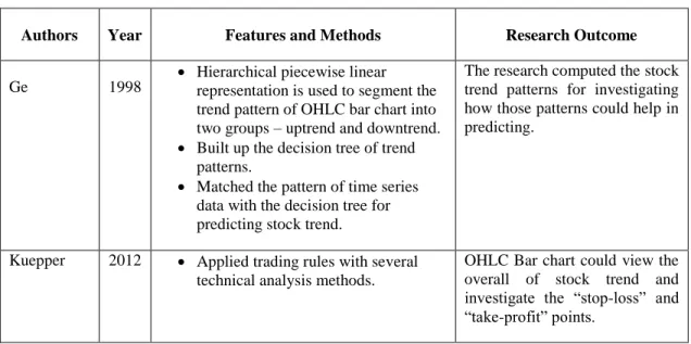
Along with Ge’s (1998) study, he introduced hierarchical piecewise linear representation to segment the trend pattern of OHLC bar chart into two groups – uptrend and downtrend, and build up the decision tree of trend patterns. Once the decision tree was done, he utilised pattern matching algorithm to match the pattern of time series data with the decision tree for predicting stock trend. This algorithm computed the probability values to certain patterns that have been occurred. He believed that the matching method could easily go up and down the hierarchy for suitable segments in decision tree that was used for predicting the trend patterns.
Another research done by Kuepper (2012) has applied the trading rules with several technical analysis methods to improve accuracy rate of prediction, and easily position the “stop-loss” and “take profit” points. He found that using the position of OHLC bar chart could assist the investors to understand the overall trend of the financial market.
23 | P a g e Table 2.2 summarises research outcome drawn by two prominent researches. These authors found that trading strategy and rules could be combined with OHLC bar chart to represent financial trends for investigating the movement direction.
Table 2.2 - Review of Financial Time Series Prediction Model using OHLC Bar Chart
Authors Year Features and Methods Research Outcome
Ge 1998
Hierarchical piecewise linear representation is used to segment the trend pattern of OHLC bar chart into two groups – uptrend and downtrend. Built up the decision tree of trend
patterns.
Matched the pattern of time series data with the decision tree for predicting stock trend.
The research computed the stock trend patterns for investigating how those patterns could help in predicting.
Kuepper 2012 Applied trading rules with several
technical analysis methods.
OHLC Bar chart could view the overall of stock trend and investigate the “stop-loss” and “take-profit” points.
As a conclusion, the candlestick pattern shows a more informative way to interpret the overall trend of financial time series compared to the OHLC bar chart. This is because the candlestick pattern utilises the RB colour to interpret the representation of open and close prices relationship for different time stamps.
24 | P a g e
2.1.2 Financial Time Series: Technical Indicators
In the financial field, the technical indicators utilise a series of data point, which are derived by applying formulas to calculate the movement of financial time series over the specified time stamp. It uses to identify the future price levels, investigate the financial trend direction and security by looking at the historical information of stock (Using Technical Indicators, 2009). Technical indicators serve for three important functions – “to alert”, “to confirm” and “to predict” (Introduction to Technical Indicators and Oscillators, 2012).
This category discusses certain technical indicators that include Exponential Moving Average (EMA), Linear Regression Line (LRL), Moving Average Convergence-Divergence (MACD) and stochastic oscillator.
Exponential Moving Average (EMA)
EMA is used to analyse and keep track of the trend changes of financial time series. It provides an element of weighting with each previous day. Furthermore, EMA can determine that a slope of financial trend is positively related with the stock price. It always decreases when price closes below the moving average of stock price and always increases when the price is increased (Exponential Moving Average, 2012). The EMA is calculated with the following equation:
25 | P a g e
(2.1)
where is defined as 2 / ( Number of days + 1).
Edward and Magee (2007) implied that EMA was relatively easy to use the equation 2.1 for calculating the predictions of stock trend. They found that EMA indicator has the power of support and resistance level to assist the investors for analysing the trend patterns based on the historical data. They also concluded that EMA indicator could show the trend for prediction easily.
Based on a research which done by Tanaka-Yamawaki et al. (2009), they utilised the pattern recognition approach that was combined with EMA to create the prediction model. In the experiment, EMA was applied to recognise the pattern of uptrend and downtrend of stock price by using a two dimension metric format, and then utilised those patterns for EMA in order to predict the price range. They had successfully improved the rate of prediction accuracy above 67%.
According to the experiment done by Dzikevicius and Saranda (2010), they found that EMA was adequate to analyse the financial trend. From their tracking signal, they concluded that EMA was less risky to identify the direction of financial trend instead of predicting the direction.
Table 2.3 summarises the experimental outcome and discussion that carried out by few authors. Each of these works successfully identifies the trend; however, it fails to capture the nonlinear pattern in data. Such approach could usually fail in predicting
26 | P a g e future trends via EMA. This method works similar to statistical methods in defining current financial trend directions.
Table 2.3 - Review of Financial Time Series Prediction Model using EMA
Authors Year Features and Methods Research Outcome
Edward and Magee
2007 Implied that EMA to calculate
direction of stock trend.
It could easily show the financial trends for prediction.
Tanaka-Yamawaki et al.
2009
Utilised the pattern recognition approach to recognise the pattern of uptrend and downtrend of stock price by using 2-dimension metric format.
Utilised those patterns for EMA in
order to predict the price range.
The rate of prediction accuracy was 67%.
Dzikevicius and Saranda
2010
Used S&P 500 and OMX Baltic Benchmark data as features. Applied buy-and-sell strategies and
specific rules with EMA. Find out the appropriate value of
Constanta to apply EMA rule.
The tracking signal result done by the authors showed that EMA can identify the financial trend with fewer errors.
Linear Regression Line (LRL)
LRL is a statistical tool that is used to calculate the slope value of regression line. A straight line is drawn through the time-series data to identify the distances between the prices of different time frame and trendlines (Linear Regression Line, 2012). The slope is used to identify two major trend patterns; a positive slope is defined as an uptrend whilst a negative slope is defined as a downtrend. The following equation defines a straight line, which is used to identify the trends over the historical data:
27 | P a g e
(2.2)
where is defined as price, is defined as slope, is defined as different period of time and is defined as intercept.
Figure 2.5 shows the basic concept of linear regression line using the equation 2.2 to identify the direction of financial trends in a certain period of time. Financial experts concluded that when the price is under the LRL (solid line shown in Figure 2.5), it is considered as buy signal, and when the price is above the LRL, it is considered as a sell signal.
Figure 2.5 - Example of Linear Regression Line 1.327 1.328 1.329 1.33 1.331 1.332 1.333 1.334 1.335 1.336 1.337 P ri ce Time
28 | P a g e Traditionally, the LRL approach has been applied to many real-world situations and the model is easy to develop and implement. Zhang (2001) explained that the limitations of price prediction based on LRL in terms of complex time series data requirement. This is because the LRL approach only analysed the trend patterns from the financial time series data. Moreover, the experiment results show that the ANN can be a satisfactory solution for complex time-series prediction.
According to Rinechart (2003), he had implemented Regression Trend Channel (RTC) technique, which includes LRL, upper trendline channel and lower trendline channel in order to analyse the trends for identifying two major trend patterns. In the experiment, he applied Pearson Correlation Coefficient to detect the desirable trend patterns which proved that LRL was working well in identifying trend patterns.
In Ahangar et al. (2010)’s paper, the trend patterns were identified using macro-economic variables and financial variables as selected features. Subsequently, the LRL approach was implemented to predict the direction of future trends. The limitations regarding price prediction based on LRL are highlighted in this paper, such as being unable to predict the price directly. Furthermore, the authors suggested combining LRL with machine learning algorithms in order to improve the prediction process. Similar work had been done by Naeini et al. (2010), which applied the lowest, highest and average value of stock market from the historical financial time series data as input features for prediction. The authors found that LRL was able to identify the direction of
29 | P a g e current and past trend changes for features extraction rather than being able to predict future trends directly.
Another research conducted by Olyaniyi et al. (2011) had fully utilised LRL to generate new knowledge from the time-series data, and successfully identified the trend patterns involved. They proved that LRL could be used as a technique to describe trend patterns for prediction purposes.
Table 2.4 summarises the research outcome of few authors. According to these findings, LRL is tip as the better approach to feature extraction. In addition, these approaches provide a useful marker to assess changes over time stamp.
Table 2.4 - Review of Financial Time Series Prediction Model using LRL
Authors Year Features and Methods Research Outcome
Zhang 2001 LRL was implemented to analysis the
trend patterns.
Utilised the patterns as input features for machine learning algorithm to predict the price.
The author explained that LRL could be a satisfactory solution for identifying the financial trends through complex time-series data.
Rinehart 2003 RTC technique – the linear regression
line, the upper trendline channel and the lower trendline channel have been applied to identify the stock trend. The Pearson’s value is used to
identify and detect the desirable stock price movement.
The author proved that the combination of RTC technique and Pearson values were fitting
well for identifying stock
trends.
Ahangar et al.
2010 Identified the trends using
macro-economic variables and financial variables are implemented as key features.
Developed the prediction model
using LRL.
The authors found that the ANN algorithm was better than LRL approach in prediction.
30 | P a g e
Naeini et al. 2010 Applied the lowest, highest and
average value of stock market from the historical financial time series data as input features.
Normalised the value of stock market
into the range [-1, 1] for ANN and LRL to predict the price.
The authors found that LRL able to identify the direction of current and past trend changes.
Olaniyi et al.
2011 LRL was implemented to generate
new knowledge from the historical stock data.
Identified the patterns that described the stock trends.
This research utilised LRL as data mining method to identify
the trend patterns from
historical data.
Moving Average Convergence-Divergence (MACD)
MACD is developed by Gerald Appel, which used to spot the changes, direction and momentum of stock trend. It consists of using two different periods of EMAs – short period EMA (12 days) and long period EMA (26 days) to identify a stock trend reversal or continuation of a stock trend, and then using a signal line to determine buy or sell the stock. The basic trading rule is to sell when the MACD line falls below the signal line (Moving Average Convergence-Divergence (MACD), 2012).
Figure 2.6 shows the example of the MACD indicator graph. The MACD histogram and line spots the divergences into “Bullish” and “Bearish”. “Bullish” divergence occurs when the MACD is making new highs while prices fail to reach new highs, which determines buy signal. “Bearish” divergence occurs in reverse, the MACD is making new lows while prices fail to reach new low that determines sell signal.
31 | P a g e
Figure 2.6 - MACD Indicator
According to Tanaka-Yamawaki and Tokoukas’ (2007) study, they mentioned that MACD did not perform well in their experiment. They had proved and concluded that MACD had to combine with other types of indicators to improve the prediction average rate up to 66%. An experiment conducted by Fernandez-Blanco et al. (2008) shown that the parameters of MACD can be implemented as a feature to improve their evolutionary algorithm for stock prediction.
Table 2.5 summarises selected research outcomes by few authors. From these findings, MACD could be utilised as the reliable feature to identify the buying and selling signals. However, MACD does not improve accuracy of prediction, as it requires certain amount of time series data to calculate and identify the trends during modelling.
32 | P a g e
Table 2.5 - Review of Financial Time Series Prediction Model using MACD
Authors Year Features and Methods Research Outcome
Tanaka-Yamawaki and Tokouka
2007 Employed genetic algorithm with
EMA and MACD as features. Generated the decision tree structure
using selected features.
The decision tree is used to predict the direction of financial trend.
The result showed that the combinations of MACD with other type of indicators had improved the accuracy rate of prediction to 66%.
Fernandez-Blanco et al
2008 Utilised MACD as input parameters
for evolutionary algorithm to develop the prediction model.
The authors proved that their prediction model that used the input parameters of MACD
could be improved with
evolutionary algorithm.
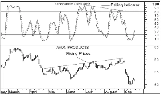
Stochastic Oscillator
Stochastic oscillator is developed by George C.Lane in the late 1950s, which used to track the momentum of stock market and gives a warning signal of the stock trend. It shows the location of current closing price that relative to the range of high and low prices over a set of time stamp. It is displayed in two lines – main line is called “%K” and the second line is called “%D” (Singh & Kumar, 2011). %K line compares the latest closing price with the recent time stamp trading. %D is a signal line calculated by smoothing %K line.
Figure 2.7 shows the concept of stochastic oscillator. The %K is displayed as a solid line and %D is displayed as a dotted line. To understand the trend rules in this indicator, the concept is defined as “buys when the %K line rises above the %D line and sells when the %K line falls below the %D line” (Achelis, 1995; Singh & Kumar, 2011).
33 | P a g e
Figure 2.7 - Stochastic Oscillator
An article which done by Ng (2007), he mentioned that stochastic oscillator has the ability to show the clear “Bullish” and “Bearish” signals. Thus, he utilised the ability of stochastic oscillator to combine with another indicator known as Guppy Multiple Moving Average (GMMA) to analyse the signals and predict the stock trend. Dharmik Team had implemented the concept of stochastic oscillator - %K and %D lines for their case studies. They utilised the %K and %D values as parameter to identify the correct time to generate profit from investment. They concluded that stochastic oscillator correctly used and followed, it can offer complex and correct information for investment (Norris, n.d.).
34 | P a g e From reviews, the LRL shows the result of analysing the financial trends in more consistent compared to other indicators approach. LRL calculates a "best-fit" line through the financial time series and provides a slope to identify the trends. It also has the ability to avoid the unbiased fit in the data.
2.2 Prediction Techniques – Artificial Intelligence (AI) Techniques
An AI technique is the study of designing computer systems, which shows characteristics that associate with intelligent human behaviour. The concept of AI technique is that a computer can be developed to assume some capabilities normally thought like human intelligence, such as adapting, self-learning and self-correction. AI research is not an easy task because a computer must be able to do many things in order to be called “Intelligent” (Kok et al., 2009).
Since 1990s, researchers from computer science sector have implemented AI techniques with technical analysis methods to develop more accurate financial time series prediction model. In this section, AI techniques will be categorised into three categories: Expert System (ES), machine learning algorithms and hybrid intelligence systems, which reviews the feature of financial trend patterns for AI techniques to learn, and the combination of technical analysis methods and AI techniques for financial time series prediction.
35 | P a g e
2.2.1 Expert System (ES)
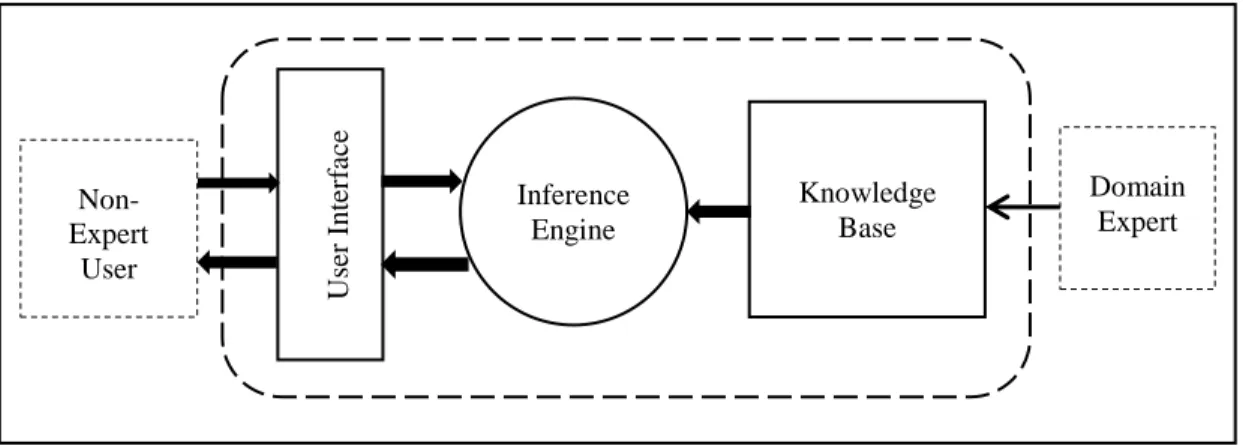
An ES is a type of computer software that mimics the behaviour and knowledge of human domain experts in specific areas, in order to provide a higher quality of decision-making and advice for users. ES has often been used to advise non-experts in situations when human domain experts are unavailable. ES operate through asking the user questions about the given problem, through which they will then supply the best answer possible to support decision making (Anjaneyulu, 1998; Butuza & Hauer, 2010).
The structure of an ES is designed in three parts: user interface, inference engine and knowledge base. A user interface allows an operator to query and receive advice from the ES. The knowledge base of ES is designed based on compiling human domain experts’ knowledge, and is transformed into rule conditions that are then used by ES. The structure of inference engine in ES is designed to produce reasoning based on the rules within the ES. The inference engine of ES will detect the contradictions within the rules and refine the problem, and it will provide the user with information, which is similar to the way of human expert’s thinking. Figure 2.8 shows the basic structure of an ES.
36 | P a g e Based on the research which conducted by Kim and Park (1996), they found that rule induction algorithm is a good solution to generate the rules in ES compared to former ES approach. They consulted domain experts for data features selection, and then categorised the data collection by using Iterative Dichotomiser 3 (ID3) approach to discover the decision tree. The casual model of ES shows the effect value based on the induced rules that had been fired, and then provides the explanation of the ES conclusion and information about the stock prediction for investors whether to accept or reject. The author found that ES does not always generate a successful explanation of the classification rules.
According to Lee and Jo’s (1999) research, they applied candlestick pattern to develop an ES to predict the timing to buy or sell stock. During the development of their ES, they had interviewed investment domain experts to create the rule-based and used candlestick pattern to visualise the stock price movement for predicting stock price. The
User I n ter fac e Inference Engine Knowledge Base Non-Expert User Domain Expert
37 | P a g e ES based on the candlestick patterns and the rule-based to predict the movement of stock price which was constructed from various patterns and suggests the information and decision of stock price to investors. They proved that candlestick pattern was very useful as the feature, and concluded that the limitation of their system was lack of automated learning.
Along with Chang and Liu’s (2008) study, they utilised stepwise regression to choose suitable selected features from six technical indexes and used k-mean method to cluster into different groups. To prove the proposed method, they setup the fuzzy rules-based with simulated annealing method to search the optimal value for rule parameters of fuzzy rules-based. They used the training data for experiment as well as to map with the most similar rules from fuzzy rules-based to predict the stock trend.
Table 2.6 summarises the research outcomes done by few authors. The limitation of ES is that the inability to offer automated learning. Reason could be that the implementation of rules is not directly applicable to constantly changing scenarios. To solve these issues, ES has to generate new rules to adapt and to solve different scenarios.
38 | P a g e
Table 2.6 - Review of Financial Time Series Prediction Model using ES
Authors Year Features and Methods Research Outcome
Kim and Park
1996 Used historical transactions data.
Interviewed with domain experts for
data collection.
Used induction algorithm (ID3) to
create decision tree.
Generated the inducted rules for explanation of the result with casual model.
The author found that ES does not always generate a successful explanation of the classification
rules. Furthermore, the
decisions for certain cases are inconsistent with the prediction of classification rules.
Lee and Jo 1999 Analysed stock data in candlestick
pattern.
Represented trading rules from
financial experts.
Collected real invested result which was used to fine tune the
knowledge.
Adjusted the knowledge after
analysed market trends from case base.
Utilised the candlestick chart as key information to develop the ES.
The experiment conducted by the authors had an average hit ratio 72% as prediction result.
Chang and Liu
2008 Utilised linear regression as selected
features.
Used stepwise regression to identify the suitable selected features, then used k-mean method to cluster the parameters into few groups. Setup the fuzzy rules-based. Used the training dataset to attempt
and map with the most similar rules to predict the stock trend.
The experiment proved that the combination of linear regression with ES has greatly improved the ability of prediction.
39 | P a g e
2.2.2 Machine Learning Algorithms
In this category, it reviews a certain machine learning algorithms such as Artificial Neural Network (ANN), Hidden Markov Model (HMM) and Support Vector Machine (SVM) that are implemented in the experiments of financial time series prediction model which conducted by researchers.
Artificial Neural Network (ANN)
ANN is a mathematical model that inspired by the neural network that forms the human brain. Human brains consist of few hundred billions of neurons, with each neuron acting as an independent biological information processing unit. This concept contributes a strong inspiration for building an intelligent neural model which known as ANN. This model functions by simulating the functioning of brain for problem solving on a computer system (Alvarez, 2006).
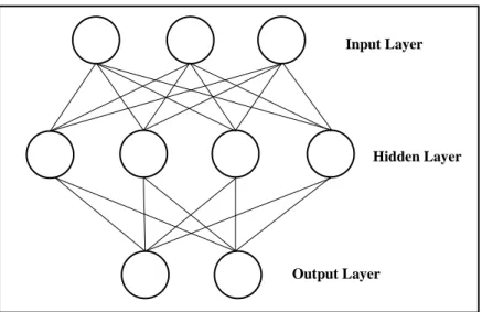
ANN acts as a black box to classify an output based on patterns recognised from a given input. Figure 2.9 illustrates the basic structure of ANN. It consists of an input layer, hidden layer and output layer. All the nodes of each layer are connected to each node in the next layer. During the learning and training process, the training inputs are presented at the input layer, with connections within the hidden layer used to acquire classification, while the desired output is presented at output layer. Moreover, ANN trains based on the given input value features, and classifies the outcomes appropriately.
40 | P a g e According to Kamijo and Tanigawa’s (1990) research, they utilised the candlestick pattern and used the extracting triangle approach to mark resistance lines on the trend pattern for recognition. The authors found that ANN is able to identify and recognise candlestick patterns in the learning and training stage. Goswamil et al. (2009) also utilised the ability of candlestick patterns as selected features to analyse the raw data of stock price and capture it in a database. Then, the authors utilised Self – Organising Map (SOM) and Case – Based Reasoning (CBR) to predict the stock price. SOM is used to train with the candlestick patterns from database, and then CBR is used to find out the best pattern matching with the new inputs (open, close, high and low prices) and existing patterns from the database to predict the short-term stock price and market timing. The authors concluded that the proposed method could identify the patterns for predicting the stock trend.
Input Layer
Hidden Layer
Output Layer
41 | P a g e Along with the experiment done by Lawrence (1997), he utilised the technical analysis method – EMH (Efficient Market Hypothesis) as feature to test with ANN for stock price prediction. Since the result of prediction model did not perform well, he concluded that feature of stock trend must be fully understood so that ANN will learn the correct pattern to predict the stock trend.
Yao and Tan (2000) proposed a prediction model that used technical indicators and financial time series data as selected features, then utilised ANN to capture the movement of currency exchange rates. The authors proved that the combination of ANN with a simple technical analysis method was a good approach for predicting exchange rates. To enhance the prediction model, they suggested that trading strategies were needed to be considered as extra features for prediction.
In Kamruzzaman and Sarkers’ (2003) first studies, they implemented the historical Forex rates and moving average as selected features for the ANN algorithm and ARIMA model to predict the future trends of exchange rates. The author concluded that the ANN algorithm could predict the exchange rates more closely than ARIMA. According to another experiment done by them, they had applied five technical indicators as selected features to identify the trend patterns of exchange rates. Then, ANN – Back propagation algorithm and Scaled Conjugate Gradient (SCG) has been implemented to develop the prediction model. In the experiment results, the authors proved that the proposed model is more capable to predict the trend direction of exchange rates closely than their previous ANN prediction model (Kamruzzaman & Sarker, 2004).