Abstract—The optimisation of a method to numerically simulate 3D velocity fields of combined wave-current flows, at individual wave resolution, is proposed. ANSYS CFX 18.0 was used to develop a homogenous multiphase model using volume fractions to define the different phase regions. By applying CFX Expression Language at the inlet of the model, Stokes 2nd Order Theory was used to define the upstream wave and current characteristics. Horizontal and vertical velocity components, as well as the surface elevation of the numerical model were compared against theoretical and experimental wave data for 3 different wave characteristics in 2 different water depths. The comparison highlighted the numerical homogeneity between the theoretical and experimental data. Therefore, this study has shown that the modelling procedure used can accurately replicate experimental testing facility flow conditions, providing a potential substitute to experimental flume or tank testing.
Keywords—ANSYS CFX; Computational Fluid Dynamics; Numerical Wave Tank; Regular Waves; Stokes 2nd Order Theory.
NOMENCLATURE
Symbol Description
−𝐶 Momentum source coefficient (kg/m3/s)
𝐶𝑎 Apparent wave celerity, stationary ref. frame (m/s)
𝐶𝑟 Relative wave celerity, moving ref. frame (m/s)
𝐻 Wave height (m) 𝐿 Wavelength (m)
𝑆𝑧 Source term in z-direction (kg/m2/s2)
𝑇𝑎 Apparent wave period, stationary ref. frame (s)
Manuscript received 12 April, 2019; revised 16 September, 2019; accepted 24 September, 2019; published 1 November, 2019. This is an open access article distributed under the terms of the Creative Commons Attribution 4.0 licence (CC BY http://creativecommons.org/licenses/by/4.0/). unrestricted use (including commercial), distribution and reproduction is permitted provided that credit is given to the original author(s) of the work, including a URI or hyperlink to the work, this public license and a copyright notice.
This article has been subject to single-blind peer review by a minimum of two reviewers.
The authors acknowledge support from SuperGen UK Centre for Marine Energy (EPSRC: EP/N020782/1) and Cardiff University for providing funding.
C. Lloyd, T. O’Doherty and A. Mason-Jones are all with Cardiff Marine Energy Research Group in the School of Engineering at Cardiff University, Queens Buildings, Cardiff, CF24 3AA, UK (email: [email protected]).
Digital Object Identifier https://doi.org/10.36688/imej.2.1-14
𝑇𝑟 Relative wave period, moving ref. frame (s)
𝑈𝑧 Measured velocity at a certain point (m/s)
𝑈𝑧,𝑠𝑝𝑒𝑐 Target fluid velocity (m/s)
𝑉 Overall volume (m3)
𝑉𝑥 Volume occupied by fluid 𝑥 (m3)
𝑊̅ Mean horizontal velocity (m/s)
𝑎 Wave amplitude (m)
𝑔 Gravitational acceleration (m/s2)
ℎ Water depth (m) 𝑘 Wave number (rad/m) 𝑟𝑥 Volume fraction of fluid 𝑥
𝑡 Time (s)
𝑣𝑎 Vertical velocity component under a wave (m/s)
𝑤𝑎 Horizontal velocity component under a wave (m/s)
𝑦 Vertical coordinate from the still water level (m)
𝑧 Horizontal coordinate in stream wise direction (m)
𝜂 Surface elevation from the still water level (m) 𝜔𝑎 Apparent angular velocity, stationary ref. frame
(rad/s)
𝜔𝑟 Relative angular velocity, moving ref. frame (rad/s)
I. INTRODUCTION
ORLD energy consumption is predicted to increase by 28% from 2015 to 2040 [1]. This increasing demand for energy coupled with environmental concerns, such as increasing Green House Gas (GHG) emissions, has sparked an interest into sources of renewable energy. Solar photovoltaic and wind energy technologies are largely developed, with a total recorded capacity in the EU at the end of 2016, of 100 GW and 154 GW respectively [2]. However, the ocean represents a highly predictable and extensive renewable energy resource which can be used to yield energy of a high quality [3] but is yet to be fully utilised. A recent study has suggested that in the UK alone, the total theoretical available energy for extraction from the tides is 216 TWh/year (91 GW) with another 69 TWh/year (27 GW) available from wave energy [4]. It is predicted by [5], that deployment of 3.4 TW of wave and tidal energy capacity could be present by 2050, with 350 TWh / year (100 GW), present in Europe.
Currently, the biggest problem with energy extraction in the marine environment, is the complex and diverse flow conditions, as detailed by [6]. Device components must be able to withstand substantial, spatial and temporal sub-surface forces generated by tidal currents, surface waves and turbulence. It is therefore important to quantify the scale of these forces prior to the design,
Development of a wave-current numerical
model using Stokes 2
nd
Order Theory
C. Lloyd, T. O’Doherty, and A. Mason-Jones
manufacture and testing of a device. Due to advances in computational processing times, the accessibility of Computational Fluid Dynamics (CFD) software, and its reduced cost in comparison to physical experimental testing, it is now possible to develop numerical models to characterise the performance characteristics of marine devices. These numerical models still require validation via the use of a Numerical Wave Tank (NWT), however the number of validation experiments is less than required for a full experimental design campaign.
A NWT is a numerical representation of a physical experimental testing facility or ocean environment. It can be used to simulate wave-current interactions using various modelling techniques within available software. Several studies detail investigations involving NWT’s.
Previous work, [7]-[8], looked at shallow water waves which, using Table I, exist at sites unsuitable for tidal energy development. Typical sea gravity waves are 1.5 – 150m in wavelength [9] and therefore, based on shallow water wave requirements, would have a water depth of <6m which is generally too shallow for turbine deployment as a water depth of 25 - 50m is the operational depth range for seabed mounted tidal devices [10]. These studies used CFD codes ANSYS CFX and OpenFoam to make comparisons between the wave elevation using Wave-Maker Theory (WMT) and the numerical model results. The sub surface particle velocities induced by the wave were not investigated in either study which would be necessary in an investigation of the loadings imparted on a tidal turbine.
Linear deep and finite depth water waves were simulated by [11], which provide a sufficient water depth for turbine deployment. A methodology for optimising the NWT was presented, and analysed the model dimensions, mesh size, time step and damping technique to dissipate the wave energy. The model also investigated wave-structure interaction and was validated against Linear Wave Theory (LWT) and WMT; although there were limitations to using WMT for the deep water wave cases. [12] expanded on this previous study to generate linear irregular waves, validated by real ocean data from the Atlantic Marine Energy Test Site (AMETS). This study was carried out using an ANSYS academic teaching license which limited mesh refinement and the associated study of simulation sensitivity to the mesh quality.
OpenFoam was also used by [13] to model regular waves in intermediate depths and gave a similar methodology for model optimisation as [11]. It was found that the simulation of regular deep water waves, with a steepness of > 0.05, experienced damping throughout the domain and were susceptible to early wave breaking, as mentioned by [8]. [14] used a Higher Order Boundary Element Method (HOBEM) to model linear and non-linear, regular and irregular waves, stating excellent agreement was achieved between the wave elevation for second order theory and the numerical results for the regular and irregular simulations.
[15] used a piston type wavemaker to generate an irregular wave train using ANSYS FLUENT, while a piston type wave maker was also used by [16], instead using OpenFoam. Active wave absorption was found to increase the stability of the system in OpenFoam and correct the problem of an increasing water level when run for long simulations.
ANSYS FLUENT was also used by [17] and [18] to generate regular waves and investigate wave-structure interaction. Initially, [17] generated regular waves and validated the model using a higher order theory, Stokes 2nd Order Theory (S2OT), before investigating the effect of waves interacting with a vertical cylinder. [17] concluded that the maximum wave height decreased in the presence of the structure and comparisons between experimental and numerical results showed good agreement. [18] developed a NWT specifically to simulate wave-current interactions in offshore environments with offshore structures. A detailed investigation into the damping domain was provided alongside a study to optimise the mesh sizing. The model enabled a calculation of the wave loads present on offshore structures under wave and current conditions. REEF3D was used in [19] to investigate wave-structure interaction with a rectangular abutment, vertical circular cylinder, submerged bar and a sloping bed. The study found the numerical model accurately measured the surface elevation of the wave and structure interaction, but the sub surface interactions were again not investigated.
[20] used S2OT to model regular, deep water waves with different wave generation methods. The mesh, time step, damping method, domain length and inlet conditions were all investigated using ANSYS CFX to give an optimised NWT model. An inlet velocity method and a piston type wavemaker were both tested and it was found that implementation of the piston type wavemaker gave better agreement with theory than when using the velocity inlet method.
This study presents 3 regular waves which were superimposed on a uniform current velocity. Each wave-current combination was modelled in 2 different depth tanks, producing deep and intermediate water depth conditions. Comparisons to the NWT were made using theory as well as experimental data obtained by the University of Liverpool [23].
This paper is organised as follows: Section 2 provides the wave theory for S2OT, Section 3 details the numerical methodology, in particular the geometry, mesh and physics setup, Section 4 discusses the main results and validation for the NWT, with Section 5 providing the main conclusions.
II. WAVE THEORY
LWT was developed by developed by Airy in 1845 [24] and provides a reasonable description of wave motion in all water depths. LWT relies on the assumption that the wave amplitude is small in comparison to the wavelength and therefore higher order terms are ignored allowing the free surface boundary condition to be linearized. If the amplitude is large then the higher order terms must be retained to get an accurate representation of wave motion [25]. These higher order theories were first developed by Stokes in 1847 [26].
The numerical model developed in this study uses Finite Amplitude theory, in particular S2OT, to model regular waves superimposed on a uniform current. Mathematically, S2OT is essentially LWT but with the 2nd order terms included. The coordinate frame is set up so that the z-axis is positive in the stream-wise direction, y-axis is in the gravity direction with 0 at the Still Water Level (SWL) and x-axis is perpendicular to the YZ plane as shown in Figure 1.
The relative depth (h/L) and wave steepness (H/L) are 2 of the main parameters that dictate the behaviour of the wave. Table I gives the relative depth bounds for deep, intermediate and shallow water waves [23], while Table II gives the appropriate theories for various wave steepness [27].
Relative depth is therefore important in defining the type of wave condition. Circular velocity orbitals arise from having an equal horizontal and vertical velocity
component. These types of orbitals are found in deep water waves and decay exponentially through the water depth. Intermediate water waves possess circular velocity orbitals near the water surface, becoming elliptical towards the seabed. This is because the vertical velocity component decays to zero at the seabed, while the horizontal component decays at the same rate as described previously. Shallow water waves possess a constant horizontal velocity component throughout the water depth, while the vertical velocity component decays to zero at the seabed. For the work presented in this paper, the relative depth conditions that represent deep and intermediate water waves were applied. The work also used S2OT to model the wave characteristics, as it is valid for waves with a greater steepness than LWT giving a bigger range of wave cases to test.
Regular waves travelling in the same direction as a uniform current will have a wave period (𝑇𝑟), angular frequency (𝜔𝑟) and wave celerity (𝐶𝑟) in a frame of reference that is moving at the same velocity as the current (𝑊̅) [27] [eq.(1)-(2)].
𝐶𝑟= 𝐿
𝑇𝑟 (1)
𝜔𝑟=2𝜋 𝑇𝑟
(2)
In a stationary frame of reference, the waves will have a wave period (𝑇𝑎), angular frequency (𝜔𝑎) and wave celerity (𝐶𝑎). These parameters are calculated as follows [28] [eq.(3)-(5)]:
1 𝑇𝑎=
1 𝑇𝑟+
𝑊̅
𝐿 (3)
𝐶𝑎= 𝐶𝑟+ 𝑊̅ (4)
𝐿 =2𝜋
𝑘 (5)
Other important parameters include the wavelength (𝐿), wave number (𝑘), wave height (𝐻) and water depth (ℎ). The wave number can be calculated from eq. (6) which is known as the Dispersion Relation [29].
𝜔𝑟2= 𝑔𝑘 𝑡𝑎𝑛ℎ(𝑘ℎ) (6)
Figure 1. Definition of wave motion (𝐿 - wavelength, 𝐻 - wave height, ℎ - water depth, 𝜂 - surface elevation, 𝑎 – wave amplitude).
TABLE I.
RELATIVE DEPTH CONDITIONS FOR DEEP, INTERMEDIATE AND SHALLOW WATER WAVES.
Relative Depth (h/L) Type of water wave
h/L > 0.5 Deep
0.04 ≤ h/L ≤ 0.5 Intermediate h/L < 0.04 Shallow
TABLE II.
THE VARIOUS REGIONS FOR GIVEN WAVE STEEPNESS. Wave Steepness (H/L) Region
When surface waves are superimposed on a uniform current, there is an interaction between these two components. The effect of the current causes the angular frequency of the waves (𝜔𝑟) to change due to the Doppler shift [30]. This change can be observed in eq. (7).
𝜔𝑟= 𝜔𝑎− 𝑘 ∙ 𝑊̅ (7)
The surface elevation (𝜂) of the wave is given by S2OT in eq. (8) [29]:
𝜂 =𝐻
2cos(𝑘𝑧 − 𝜔𝑎𝑡) + 𝜋𝐻2
𝐿
cosh 𝑘ℎ 𝑠𝑖𝑛ℎ3𝑘ℎ(2 + cosh 2𝑘ℎ) 𝑐𝑜𝑠2(𝑘𝑧 − 𝜔𝑎𝑡)
(8)
where the amplitude (𝑎) of the wave is 𝐻2.
Surface gravity waves induce orbital velocities in the horizontal (𝑤𝑎) and vertical (𝑣𝑎) direction to the path of wave propagation. These sub surface oscillations can penetrate the water column by up to half the wavelength [28], although this can be deeper. The oscillations decay exponentially and so for engineering applications, the half wavelength estimation is considered satisfactory. The sub surface velocities can be calculated in a stationary frame of reference using eq. (9)-(10) [29].
𝑤𝑎 = 𝑊̅ +𝐻
2𝜔𝑟
cosh 𝑘(ℎ + 𝑦)
sinh(𝑘ℎ) cos(𝑘𝑧 − 𝜔𝑎𝑡)
+3 4[
𝜋𝐻 𝐿 ]
2
𝐶𝑟 cosh 2𝑘(ℎ + 𝑦)
sinh4(𝑘ℎ) cos(2𝑘𝑧 − 2𝜔𝑎𝑡)
(9)
𝑣𝑎 =𝐻
2𝜔𝑟
sinh 𝑘(ℎ + 𝑦)
sinh(𝑘ℎ) sin(𝑘𝑧 − 𝜔𝑎𝑡)
+3 4[
𝜋𝐻 𝐿 ]
2 𝐶𝑟
sinh 2𝑘(ℎ + 𝑦)
sinh4(𝑘ℎ) sin(2𝑘𝑧 − 2𝜔𝑎𝑡)
(10)
III. NUMERICAL METHODOLOGY
The NWT used in this study was set up to replicate the University of Liverpool’s recirculating water channel to enable a direct comparison between numerical and experimental results. The model dimensions were optimised for each simulation and were dependent upon the wave characteristic and water depth of the facility. The geometry and mesh were created using ANSYS ICEM 18.0 [31] while the physics setup, solver and results were all produced using ANSYS CFX 18.0 [32]. The model development has been split up into 3 main sections: 1) Geometry, 2) Mesh and 3) Physics Setup.
1) Geometry
The working section of the University of Liverpool’s recirculating water channel is 1.4m wide, 0.76m deep and 3.7m long, as shown in Figure 2 [23], but the NWT was adapted for computational reasons to have a width of
0.1m, height of 1.09m (3.5m in deep water wave conditions) and a length of 20m. The width of the domain was limited to 0.1m to reduce the overall size of the model and therefore the computational effort needed to run the model. Section 4.3 shows that this reduced width had no effect on the flow characteristics. The height of the NWT was calculated so that the SWL was at 70% of the overall height, as recommended by [11]. This meant that the overall height, of 1.09m in intermediate conditions and 3.5m in deep conditions, allowed for a water depth of 0.76m or 2.5m respectively, with an area at the top of the tank for the air. This enabled a multiphase flow model to be used which will be discussed in Section 3.3. The length of the NWT was extended to 20m to allow for 8-10 waves to propagate before reaching the end of the model as well as enabling a numerical beach of twice the wavelength (2L) to be incorporated as recommended by [33]. These settings allowed the desired wave-current characteristics to be present in a known region of the model.
2) Mesh
The mesh was developed using a ‘top down blocking strategy’ to create a structured HEXA mesh. 6 different HEXA meshes were created for a mesh independence study to ensure the mesh was refined to an acceptable level without compromising accuracy or being too computationally expensive.
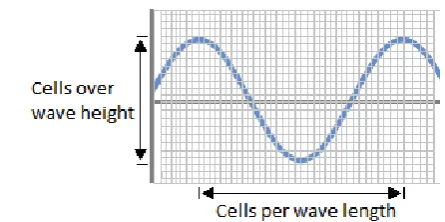
Mesh optimisation is particularly important for free surface modelling, to enhance results and reduce computational effort. When modelling a NWT, there must be an increased mesh resolution at the fluid interface. This region must capture the entire wave height to maintain the desired surface resolution at all points along the wavelength. The meshing methods used are specified in terms of the number of cells over the wave height and the number of cells per wavelength so that they can be adapted for different wave cases. Figure 3 provides an example of how these mesh definitions apply.
It is recommended by [33] to use at least 10 cells over the height of the wave and at least 100 cells over the length of a single wave which agrees with the findings of [21]. It is suggested by [11] that an element size of 1/10th of the wave height is sufficient, while [34] states that 16 cells per wave height and 100 cells per wavelength produce mesh independent results. A summary of these results are shown in Table III.
Table IV shows the settings used in comparing 6 different meshing techniques based upon the findings of [11], [21], [33], [34]. It is important to note that only HEXA meshing was investigated in this study. This is because less computational points are needed than a tetrahedral mesh, giving a higher spatial resolution with a better mesh aspect ratio increasing the accuracy of the simulation [34]. It also allows refinement of the mesh in the direction normal to the free surface without causing distortion in the other directions. This study had access to ANSYS CFX research licenses, and so the mesh was not restricted in size, unlike the study detailed in [12].
3) Physics setup
ANSYS CFX 18.0 uses the Finite Volume Method (FVM) to discretise and solve the governing equations iteratively for small sub-divisions of the region of interest. This gives an approximation of each variable at points
throughout the domain and so a picture of the full flow characteristic can be obtained [35]. The governing equations solved by the ANSYS CFX solver are the mass continuity and the Stokes equations. The Navier-Stokes equations are closed using the Shear Stress Transport (SST) turbulence model in order to resolve the flow conditions. Derivations of these equations and further information can be found in [36].
The analysis is set up as a transient run using the time step found previously, 50 divisions per wave period (T/50). Previous studies have compared the influence of 3 different turbulence models on the generation and propagation of regular waves (laminar, k-epsilon (k-ε) and the SST turbulence model) with no significant difference between each case [7], [11], [12], [37]; hence the SST turbulence model was applied in this study. The SST turbulence model is recommended for accurate boundary layer simulations [38], which is necessary in general turbine modelling and so it was used with foresight to investigate the wave-current interaction with one or more tidal turbines in future work.
The following assumptions were made when defining the domain:
1) The air is defined with a density of 1.185 kg/m³ 2) The water is defined with a density of 997 kg/ m³ 3) The surface tension at the air-water interface is
negligible
4) There is an initial hydrostatic pressure in the ‘water’ region and an atmospheric pressure in the ‘air’ region with this region being initially static
5) The seabed is horizontal and impermeable
The boundary conditions for this model were set as shown in Figure 4. The inlet was set as an ‘opening’ to allow flow into and out of the domain. This is necessary to prevent the model crashing as the horizontal and vertical velocities specified at the inlet, can produce back flow. The outlet was also set as an ‘opening’ to allow bidirectional flow. A hydrostatic pressure was used over the water depth up to the SWL as defined in Figure 1. The top of the domain was specified as an ‘opening’ with the air at atmospheric pressure. The two adjacent side walls were set as ‘free-slip wall’ so that shear stress at the wall was zero and the velocity of the fluid near the wall was not slowed by frictional effects. The base of the NWT was specified as ‘no-slip’ to model the frictional effects felt at the base of the tank. A summary of these boundary conditions are shown in Table V.
Figure 3. Mesh description definitions (grid resolution and wave surface line not to scale).
TABLE III.
RECOMMENDED MESH SETTINGS FOR FREE SURFACE MODELLING. Author
Cells over wave height (H/∆𝒚)
Cells per wavelength (L/∆𝒛) Finnegan & Goggins [11] 10 - ANSYS Inc [33] 10-20 >100
Silva et al [21] 10 145
Raval [34] 16 100
TABLE IV.
A SUMMARY OF THE DIFFERENT MESH SET-UPS. Mesh
Number
Cells over wave height (H/∆𝒚)
Cells per wavelength (L/∆𝒛)
Total Elements (thousands)
1 10 60 378
2 10 80 488
3 10 100 620
4 10 120 730
5 10 140 839
6 20 100 1140
A numerical beach was used to dampen out the waves and prevent any reflection from the end of the model. This was applied as a ‘subdomain’ over the whole model using expressions generated by CFX Expression Language (CEL) [35], to target a distance 2L before the outlet. The mesh was also gradually increased in size, making it coarser, in this region as recommended by [33]. The numerical beach was created by using a general momentum source acting in the stream wise direction. In this application, it was used to force the velocity in the beach region to be the same as the current velocity, removing the oscillatory effects of the wave. This was achieved by using eq. (11):
𝑆𝑧= −𝐶(𝑈𝑧− 𝑈𝑧,𝑠𝑝𝑒𝑐) (11)
Where 𝑆𝑧 is the source term in the z-direction, −𝐶 is the momentum source coefficient and should be set to a large number (eg. 10⁵ kg/m³/s), 𝑈𝑧 is the measured velocity at a certain point and 𝑈𝑧,𝑠𝑝𝑒𝑐 is the target velocity [35].
A homogenous multiphase model was used to model the free surface flow and is necessary when there is more than one fluid present. In this model, the 2 phases used were water and air. Volume fractions of each fluid are given by eq. (12):
𝑉1= 𝑟1𝑉 (12)
Where 𝑟1 is the volume fraction of fluid 1, and 𝑉1 is the volume occupied by fluid 1 in an overall volume, 𝑉 [39]. The volume fraction advection scheme, for free surface flows, is controlled by interface compression [35]. This in turn controls the interface sharpness and is set at a setting of 2 for ‘aggressive compression’. ‘Multiphase Control’ is activated in the ‘Solver Control’ setup, using ‘Segregated’ for Volume Fraction Coupling and ‘Volume-Weighted’ for Initial Volume Fraction Smoothing.
The NWT was tested using the wave characteristics presented in Table VI. The tests were run so that each wave case was tested in 2 different water depths, h = 0.76m and h = 2.5m. Waves 1 & 2 are both classified as
S2OT waves, and Wave 3 as a linear wave, as explained in Table II.
Each test began by having current only flow, using the uniform current velocity specified in Table VI. This was to allow the current flow to establish before the wave conditions were superimposed on top. The horizontal velocity was specified at the inlet using cartesian velocity components. After 2 seconds of run time, the wave case was superimposed onto the uniform current and run for a total time of over 100 seconds. Equations for the horizontal and vertical velocity components were input using CEL [35] at the inlet. Equations (9) and (10) were used and are described further in Section 2. The free surface interface was controlled using volume fractions to differentiate between the ‘water’ and ‘air’ regions. These volume fractions are controlled by the surface elevation of the wave as detailed in equation (8).
Stability in the model occurred after 60 – 70 seconds and so all results reported in this study were taken over a 10 second period after 70 seconds of run time. Monitor points were added into the model to observe changes through the water depth in the velocity and wave period. The deep water cases were monitored every 0.2m between y = -0.1m and y = -1.5m, while the intermediate cases were monitored every 0.1m between y = -0.12m and y = -0.62m at various locations downstream of the inlet as shown in Figure 1.
These simulations all used ‘Double Precision’ when defining the run. This setting permits more accurate numerical mathematical operations and can improve convergence. It is recommended for all multiphase modelling [35]. This work was carried out using parallel processing, specifically 32 processors over 2 nodes, using the computational facilities of the Advanced Research Computing @ Cardiff (ARCCA) Division, Cardiff University. When running in parallel, the free surface may not be robust if any portion of a partition boundary is aligned with the free surface. Therefore, ‘user specified direction’ was selected to restrict partitioning to the x and z directions only, and not in the y direction.
IV. RESULTS AND DISCUSSION
1) Mesh independence study
The horizontal and vertical velocities of the wave-current interaction were compared between the numerical model and theoretical data. Figure 5 shows the normalized horizontal and vertical velocities at various TABLE V.
BOUNDARY CONDITION DETAILS. Boundary Boundary Condition
inlet Velocity-inlet (opening) outlet Pressure-outlet (opening)
top Pressure-opening
base No-slip wall walls Free-slip wall
TABLE VI.
WAVE CHARACTERISTICS USED. Wave
Name
Depth conditions
Water Depth h (m)
H (m)
Tr (s)
𝑾 ̅̅̅
(m/s) L (m)
Steepness H/L
Relative Depth h/L
Wave 1 Intermediate 0.76 0.058 1.218 0.93 2.250 2.315
0.026 0.338
Deep 2.5 0.025 1.080
Wave 2 Intermediate 0.76 0.082 1.147 0.93 2.020 2.052
0.041 0.377
Deep 2.5 0.040 1.220
Wave 3 Intermediate 0.76 0.01 1.218 0.1 2.250 2.315
0.0044 0.338
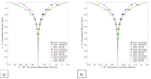
points through a water depth of 0.76 m for Wave 1, superimposed on a current, with the following properties: T = 1.218s, H = 0.058m, 𝑊̅ = 0.93m/s.
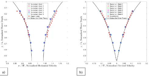
The difference between each numerical model and the equivalent theory were within 1% for the horizontal velocities and 25% for the vertical velocities. 25% may sound significant, however because the vertical velocities were so small, the differences were insignificant compared to the streamwise velocities. This was not an issue here as this study was looking at how comparable 6 different meshes were to theory and therefore the difference relative to theory is what was important here.
Looking into more detail, mesh 4 gave the closest agreement to theory for the horizontal velocity results as shown in Figure 5a. The maximum difference between
the numerical and theoretical horizontal velocities was 0.7%. Mesh 6 displayed the biggest differences with up to 1% which was similar to the errors seen in meshes 1 & 2. All the results had better agreement with theory towards the base of the tank, with bigger divergence seen towards the water surface.
Looking at the minimum vertical velocities shown in Figure 5b, mesh 3 gave the best agreement for all points through the water depth with a maximum difference between the numerical and theoretical minimum vertical velocities of 21%. Meshes 4, 5 and 6 all predicted the maximum vertical velocities extremely well, all being within 4% of one another.
After analysing all these results, meshes 1, 2 and 6 were outperformed by meshes 3, 4 and 5. Mesh 3 gave good
Figure 5. Normalised results for the numerical, theoretical and experimental maximum and minimum wave-induced: (a) horizontal and; (b) vertical velocities.
a)
b)
Figure 6. Final mesh selection using 120 cells per wavelength and 10 cells over the wave height: (a) in the XY plane; (b) in the YZ plane.
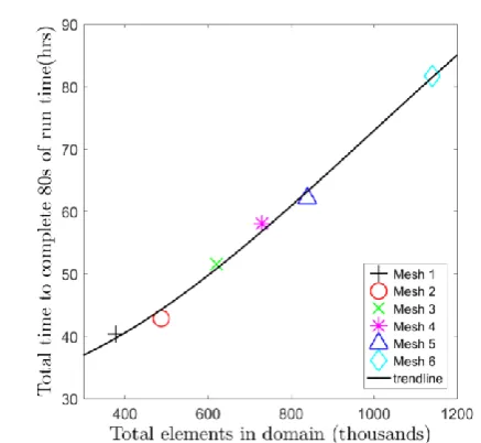
agreement for the vertical velocity results but performed less well with the more crucial horizontal velocity results. Meshes 4 and 5 had generally good agreement with the horizontal and vertical theoretical velocities, and realistically both would have performed well in the type of simulations they were required for. Figure 7 shows the total time taken to complete 80s of run time for each of the different meshes with different sized domains. Mesh 4 was computationally faster than mesh 5 by about 10%, and considering they gave marginal differences in accuracy, mesh 4 was chosen. This selection agreed with the findings shown in Table III.
Figure 6 shows the final mesh selection for Wave 1, using 10 cells over the wave height and 120 cells per wavelength. Table VII gives the specific size details for each mesh used based on the general specification previously detailed. The maximum aspect ratio of the mesh is defined as a measure of how much the mesh elements are stretched. Each mesh had a maximum aspect ratio of < 1000 which is the maximum value specified by [35], for models running in ‘double precision’ mode.
2) Time step study
The ANSYS CFX solver uses an implicit solution method and so it is recommended by [32] to resolve the physical timescales in the model by using a time step to control the simulation. It is not recommended to adopt the Courant number criterion as other CFD software might do [8], [19]. Therefore, a time step study was carried out, using the mesh description of mesh 4, to look at the effect it had on computational effort and accuracy. The time step was specified in terms of the wave period and by dividing this into a certain amount of divisions, eg. T/50. Divisions of 30, 50, 80 and 100 were investigated. Comparing the results for the horizontal velocity, as shown in Figure 9a, the models with divisions of T/50, T/80 and T/100 were all within 0.6% of each other, while T/30 showed bigger differences with a divergence of up to 2% from the theoretical velocity at the point nearest the water surface. Figure 9b shows the results for the vertical velocity comparison and T/80 gave the best agreement to theory with a maximum difference of 18% in comparison to T/30 with 33%. However, again, T/50 and T/100 were both within 3% of T/80 and so shows little difference in accuracy between these time steps.
TABLE VII. MESH SIZING PARAMETERS.
Wave Name Wave 1 Wave 2 Wave 3
Water depth (m) 0.76 2.5 0.76 2.5 0.76 2.5 Region around
air-water interface
∆𝒚 (m) 0.006 0.006 0.009 0.009 0.001 0.001
∆𝒛 (m) 0.019 0.019 0.017 0.017 0.019 0.019
∆𝒙 (m) 0.014 0.014 0.014 0.014 0.014 0.014 Mesh expansion from
interface towards the top
∆𝒚 (m) 0.010.07 0.010.18 0.010.07 0.010.12 0.010.07 0.010.16 Mesh expansion from
interface towards the base
∆𝒚 (m) 0.012 0.010.02 0.012 0.010.02 0.012 0.010.02 Mesh expansion in
beach region ∆𝒛 (m)
0.030.01
3 0.030.013 0.030.013 0.030.013 0.030.013 0.030.013 Maximum aspect ratio 21 22 16 16 127 114 Total elements (millions) 0.73 1.8 0.75 2.0 1.0 1.7
Figure 8. Computational speed of numerical model with different time steps.
It is clear to see that there was a considerable increase in accuracy between T/30 and T/50, however above 50 divisions little difference in accuracy was noted. Figure 8 shows the total time taken for the models to complete 80s of run time compared to the time step used. The smaller the time step used, the more computationally expensive the model was. This equated to a 60% increase in time between using T/50 and T/80, and 160% between T/50 and T/100. Therefore, a time step size of 50 divisions per wave period (T/50) was chosen. This agreed closely with the findings of [21] who used a time step size of T/100 , [14] who found T/40 was the maximum time step that could
be used before numerical instability occurred, and [11] who stated that the optimum time step interval was T/50.
3) Verification of reduced width NWT
The choice to use a restricted width of 0.1m instead of the full width of the experimental facility (1.4m) was made to simplify the model and increase the speed that each model would take to run. This decision was validated by measuring the horizontal and vertical velocities in the numerical model for current only conditions. The average horizontal and vertical velocities for the experimental testing results were 0.93 m/s and 0
Figure 9. Normalized results for the numerical, theoretical and experimental maximum and minimum wave-induced: (a) horizontal and; (b) vertical velocities for different time steps.
a)
b)
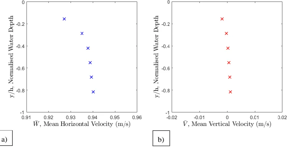
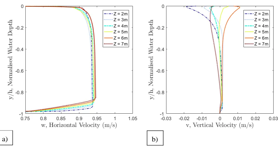
Figure 10. Averaged normalized: a) horizontal and; b) vertical velocities for current only flow through the water depth over 60s of converged run time.
m/s respectively for the Wave 1 case. Therefore, the numerical model was monitored to see if these same current conditions were being generated. Figure 10 shows the average horizontal and vertical velocities at 6 points through the water depth over 60 seconds of converged run time. The point nearest the surface deviates the most from the average horizontal and vertical experimental current velocity, showing a difference of 1% and 0.1% respectively. The depth averaged velocity of all the points gave 0.9376 m/s in the horizontal direction and 0.00016 m/s in the vertical direction. Figure 11 again shows the average horizontal and vertical velocities through the water depth, but instead for 6 different locations, a distance of 2 to 7m downstream of the inlet. A full depth profile can be seen here, with a reduction in velocity near the base of the tank and at the water surface. This is the standard profile that would be expected. Excluding the top and bottom 10% of the water depth, to find the average velocity in the main body of the flow, the average horizontal velocity was 0.9376 m/s and the average vertical velocity was -0.00015 m/s. These position averaged results agree with the time averaged velocities, showing that the average velocity was stationary, over time and in the area between 2 and 7m downstream of the inlet. Both sets of results were also within the ± 1% uncertainty of the experimental results, which is given when taking measurements using an Acoustic Doppler Velocimeter (ADV) [23]. Therefore, the decision to use a width of 0.1m instead of 1.4m was justified, to reduce computational run times without affecting the accuracy of the numerical simulations.
4) Deep water wave conditions
The following results are for deep water wave cases, modelled with a water depth of h = 2.5m. Figure 12 shows
that good agreement was found between the numerical and theoretical surface elevation for each wave case. The difference between the numerical and theoretical results for the wave height were 13%, 6% & 5% for Waves 1, 2 & 3 respectively. Marginally bigger differences occur in the trough region of the wave, in comparison to the peak. These percentages are relatively high, however, this study focusses on the sub surface conditions and accuracy of the surface elevation is not the primary concern. The average wave period (𝑇𝑎) of the numerical models were 0.818s (W1), 0.755s (W2) & 1.155s (W3) which agreed exactly with the theoretical values input to the model.
Figure 13 shows the horizontal and vertical velocities through the water depth for the numerical and theoretical results. Comparing the horizontal velocities, the maximum difference between the numerical results and theory was 1.3%. Wave 1 showed the smallest differences with a maximum of 0.8%. The numerical results for the vertical velocities showed a maximum difference to the
Figure 12. Surface elevation of Wave 1, 2 & 3 in deep water conditions at location 4m downstream of inlet.
Figure 11. Normalised: a) horizontal and; b) vertical velocities for current only flow through the water depth at 6 different locations on the z-axis at T=80s.
theory of 41%. This percentage seems high, however, the raw values at this point, nearest the base of the tank, gave -0.0026 m/s for the numerical model and -0.00438 m/s for theory. Therefore, the raw difference between these two values was 0.0018 m/s which is very small, but as a percentage of the theoretical value, has a greater magnitude. The raw difference observed between the theory and the numerical results near the water surface was in fact greater at 0.0113 m/s, but as a percentage of the theory gives 5.8% which is smaller. The magnitude of the velocity at the surface is greater than that towards the base even though the percentage difference demonstrates otherwise. So intuitively, care must be taken when studying these effects. Wave 2 showed the smallest differences in vertical velocity with a maximum of 19%.
These results have shown that there was very good agreement between the numerical velocity results and the theoretical data produced using S2OT. It is therefore reasonable to state that this type of NWT is capable of providing a good estimation of the sub surface velocities for deep water wave-current conditions.
Due to the relative depth (h/L) of these deep water wave cases, it can be seen that the velocity fluctuations are minimal half way down the water column, with oscillations decaying completely by the time they reach the bottom of the tank. Therefore, if a marine device was placed in the bottom half of the water depth it would encounter minimal velocity variations while still being able to extract energy from the dominating current flow. For certain deployment sites with devices positioned in an area of relatively uniform flow, this type of model could be used to gather information on the flow characteristics present in relatively steady flow regions.
For other sites with highly sheared flow conditions, a profiled flow model would be more appropriate [40].
5) Intermediate water wave conditions
The following results are for intermediate water wave cases, modelled with a water depth of h = 0.76m. All wave cases were compared to theory, with wave cases 1 & 2 also being compared to experimental results obtained by the University of Liverpool. The experimental results obtained by the University of Liverpool were collected over 250 wave cycles and averaged to determine the mean wave profiles. It was found that the wave height could vary by ±5% and the wave period by ±0.5%. The vertical and horizontal velocities were measured using an Acoustic Doppler Velocimeter (ADV), which gave the results an uncertainty of ±1%. The ADV covered a depth range from y = -0.12m to y = -0.42m with y = 0m being at the SWL [23].
Figure 13. The normalized a) horizontal and; b) vertical velocities at monitor points through the water depth at a location 4m downstream of the inlet for numerical results and S2OT.
a)
b)
Figure 14 shows the numerical and theoretical surface elevation for each wave case at an intermediate depth. The maximum difference between the experimental and theoretical wave height for Waves 1, 2 & 3 was 3%, 6% and 2% respectively. Waves 1 and 3 are therefore within the ±5% of the wave height variation found experimentally, with Wave 2 just outside this region. The overall wave height may agree with the experimental and theoretical wave heights, however, there is a slight shift vertically with the numerical results in comparison. As mentioned before, the sub surface velocities are of more interest as long as the surface elevation is reasonably accurate. The same errors are apparent when compared to the theoretical results as these average results are the same as the experimental. The average wave period (𝑇𝑎) of the numerical models was 0.81s (W1), 0.75s (W2) & 1.15s (W3) which again agreed precisely with the theoretical values input to the model. Again, the experimental results were the same as the theory and so these results also showed good agreement with the average wave period for each wave case.
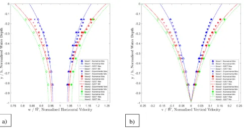
The horizontal and vertical velocities, at points through the water depth, given by the numerical model, theory and experimental testing are shown in Figure 15. The numerical results in the horizontal direction showed good agreement with both the experimental and theoretical data. The maximum % difference between the horizontal numerical results and theory was 1.5%, with a marginally higher difference of 2.2% between the numerical results and the experimental. The numerical horizontal velocity for Wave 1 showed better agreement with theory having a difference of < 0.7%, in comparison to the experimental results with < 2.2%. This was because, as the experimental results got closer to the water surface, the results diverged. Numerical horizontal velocities for
Waves 2 and 3 both showed < 1.5% difference to the theory, with these biggest differences shown towards the water surface where oscillatory motions induced by the wave were the greatest. Comparing numerical results for Wave 2 against the experimental data also showed differences of < 1.5% with similar greater differences shown near the water surface.
The maximum % differences between the vertical numerical results, with theory and experimental data, were 22% and 16% respectively. The biggest divergence observed with these results were seen near the water surface for the maximum vertical velocities, yet near the base of the tank for the minimum vertical velocities. Even still, these numerical results follow the main trends shown in the theoretical and experimental data, giving a good representation of the sub surface wave and current interactions for intermediate water depths.
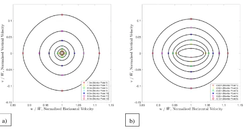
It was clear to see that the horizontal velocities of the intermediate water conditions still had a considerable oscillatory effect near the bottom of the tank in comparison to the vertical velocities, which tended to zero at the bottom of the tank. This causes the shape of the velocity orbitals to be more circular near the surface of the water and become elliptical towards the bottom of the tank. This can be seen in Figure 16 where the normalised maximum and minimum, horizontal and vertical velocities have been plotted for Wave 1, to give an estimation of the shapes and sizes of the Eulerian velocity history for different depths through the water column. This is different to the deep water wave conditions where both the horizontal and vertical velocities tended to zero at the bottom of the tank. It can be seen from Figure 16 that the orbitals are much more circular for the deep water wave case than the intermediate water wave case. These results are what
Figure 15. The normalised a) horizontal and; b) vertical velocities at monitor points through the water depth at a location 4m downstream of the inlet for numerical results, experimental results and S2OT.
would be expected for deep and intermediate water wave conditions.
The mesh selection was extremely important in enabling the numerical model to have good agreement with the theoretical and experimental results. This study, however, only looked at using a HEXA mesh to create the NWT and other meshing techniques could be further investigated. Validation of this NWT has been achieved using S2OT and experimental results using 3 different wave cases in 2 different depth tanks. The 6 tests were modelled over a broad area of theories as well as intermediate and deep water conditions. This model could be tested further by using Stokes 3rd, 4th or 5th Order Theories to test waves with larger amplitudes. Further work will build upon this set of guidelines for wave-current modelling and develop a profiled flow model giving a broader range of wave-current conditions that can be tested.
V. CONCLUSION
The aim of this study was to develop a NWT to simulate the wave-current interaction between regular waves and a uniform current velocity, but more specifically to study sub surface conditions. To do this, 6 simulations were carried out using 3 different wave characteristics and 2 different depth tanks. The regular wave cases were all within the S2OT and linear wave regions. Guidelines for the development of an optimum NWT have been established, detailing the importance of mesh development and model setup. For an engineering application, the optimum mesh size and time step was found to have 10 cells over the wave height and 120 cells per wavelength with a time step of T/50. The model was set up as a homogenous multiphase model using volume
fractions to differentiate between fluid phases. Numerical results for all 6 simulations were in good agreement with theoretical and experimental results. Finally, this study has shown that numerical models can effectively replicate wave and current experimental data, for the conditions shown, and therefore provides a valid contribution to literature, presenting a cheaper alternative to physical design and experimental testing.
The wave and current cases used in this study present a simplified case by using a uniform current flow and regular surface waves. Further development of the numerical model would look to emulate more realistic, ocean flow regimes by generating flow conditions with a higher complexity. This would include using sheared velocity profiles and modelling waves oblique to the current.
ACKNOWLEDGEMENTS
This work was carried out using the computational facilities of the Advanced Research Computing @ Cardiff (ARCCA) Division, Cardiff University. The authors would also like to thank the University of Liverpool for providing experimental data.
REFERENCES
[1] U.S Energy Information Administration, “International Energy Outlook 2017,” 2017.
[2] European Commission, Strategic Energy Technology Plan. 2017.
[3] M. Lewis et al., “Power variability of tidal-stream energy and implications for electricity supply,” Energy, vol. 183, pp. 1061–1074, Sep. 2019.
[4] The Crown Estate, “UK Wave and Tidal Key Resource Areas Project,” 2012.
[5] Ocean Energy Europe, “Ocean energy project spotlight: Investing in tidal and wave energy,” 2017.
Figure 16. Normalised maximum and minimum, horizontal and vertical velocities to give an idea of the shape and magnitude of the velocity orbitals for a) deep and; b) intermediate water wave conditions for Wave 1.
[6] A. Alberello, A. Chabchoub, O. Gramstad, A. V Babanin, and A. Toffoli, “Non-Gaussian properties of second-order wave orbital velocity,” Coast. Eng., vol. 110, pp. 42–49, 2016. [7] A. Lal and M. Elangovan, “CFD Simulation and Validation
of Flap Type Wave-Maker,” Int. J. Math. Comput. Sci., vol. 2, no. 10, pp. 708–714, 2008.
[8] N. Jacobsen, D. Fuhrman, and J. Fredsøe, “A wave generation toolbox for the open-source CFD library: OpenFoam,” Int. J. Numer. Methods Fluids, vol. 70, no. 9, pp. 1073–1088, 2012.
[9] A. Toffoli and E. M. Bitner-Gregersen, “Types of Ocean Surface Waves, Wave Classification,” Encycl. Marit. Offshore Eng., pp. 1–8, 2017.
[10] A. S. Iyer, S. J. Couch, G. P. Harrison, and A. R. Wallace, “Variability and phasing of tidal current energy around the United Kingdom,” Renew. Energy, 2013.
[11] W. Finnegan and J. Goggins, “Numerical Simulation of Linear Water Waves and Wave-Structure Interaction,” Ocean Eng., vol. 43, pp. 23–31, 2012.
[12] W. Finnegan and J. Goggins, “Linear irregular wave generation in a numerical wave tank,” Phys. Procedia, vol. 52, pp. 188–200, 2015.
[13] R. J. Lambert, “Development of a numerical wave tank using OpenFOAM,” University of Coimbra, 2012. [14] D. Ning and B. Teng, “Numerical simulation of fully
nonlinear irregular wave tank in three dimension,” Int. J. Numer. Methods Fluids, no. November 2006, pp. 1847–1862, 2007.
[15] X.-F. Liang, J.-M. Yang, J. Li, X. Long-Fei, and L. Xin, “Numerical Simulation of Irregular Wave - Simulating Irregular Wave Train,” J. Hydrodyn., vol. 22, no. 4, pp. 537– 545, 2010.
[16] P. Higuera, J. L. Lara, and I. J. Losada, “Realistic wave generation and active wave absorption for Navier-Stokes models Application to OpenFOAM®,” 2013.
[17] X. Tian, Q. Wang, G. Liu, W. Deng, and Z. Gao, “Numerical and experimental studies on a three-dimensional numerical wave tank,” IEEE Access, vol. 3536, no. c, pp. 1–1, 2018. [18] S.-Y. Kim, K.-M. Kim, J.-C. Park, G.-M. Jeon, and H.-H.
Chun, “Numerical simulation of wave and current interaction with a fixed offshore substructure-NC-ND license (http://creativecommons.org/licenses/by-nc-nd/4.0/),” 2016.
[19] H. Bihs, A. Kamath, A. Chella, A. Aggarwal, and Ø. A. Arntsen, “A new level set numerical wave tank with improved density interpolation for complex wave hydrodynamics,” Comput. Fluids, vol. 140, no. 7491, pp. 191–208, 2016.
[20] F. M. Marques Machado, A. M. Gameiro Lopes, and A. D. Ferreira, “Numerical simulation of regular waves: Optimization of a numerical wave tank,” Ocean Eng., vol. 170, pp. 89–99, Dec. 2018.
[21] M. C. Silva, M. A. Vitola, P. T. T. Esperanca, S. H. Sphaier, and C. A. Levi, “Numerical simulations of wave-current flow in an ocean basin,” Appl. Ocean Res., vol. 61, pp. 32–41, 2016.
[22] S. F. Sufian, M. Li, and B. A. O’Connor, “3D Modeling of Impacts from Waves on Tidal Turbine Wake Characteristics and Energy Output,” Renew. Energy, pp. 1–15, 2017. [23] T. D. J. Henriques, T. S. Hedges, I. Owen, and R. J. Poole,
“The influence of blade pitch angle on the performance of a model horizontal axis tidal stream turbine operating under wave-current interaction,” Energy, vol. 102, pp. 166–175, 2016.
[24] G. B. Airy, “Tides and Waves,” Encycl. Metrop., vol. 5, pp. 341–396, 1845.
[25] V. Sundar, Ocean Wave Mechanics: Applications in Marine Structures. London: Wiley, 2016.
[26] G. G. Stokes, “On the theory of oscillatory waves,” Trans. Cambridge Philos. Soc., vol. 8, pp. 441–455, 1847.
[27] T. S. Hedges, “Regions of validity of analytical wave theories,” Proc. Inst. Civ. Eng. - Water Marit. Eng., vol. 112, no. 2, pp. 111–114, 1995.
[28] R. Sorensen, Basic Coastal Engineering, 3rd ed. Pensylvania: John Wiley & Sons, 2006.
[29] J. S. Mani, Coastal Hydrodynamics. New Delhi: PHI Learning Private Limited, 2012.
[30] P. W. Galloway, L. E. Myers, and A. S. Bahaj, “Studies of a scale tidal turbine in close proximity to waves,” 3rd Int. Conf. Ocean Energy, Bilbao, Spain, 6 Oct 2010, no. 1, pp. 3–8, 2010.
[31] ANSYS Inc, “ANSYS ICEM.” Release 18.0. [32] ANSYS Inc, “ANSYS CFX.” Release 18.0.
[33] ANSYS Inc., “ANSYS Fluent Advanced Workshop: Simulation of Small Floating Objects in Wavy Environment with ANSYS Fluent,” 2016.
[34] A. Raval, “Numerical Simulation of Water Waves using Navier-Stokes Equations,” PhD Thesis, University of Leeds, 2008.
[35] ANSYS Inc, “ANSYS CFX Modelling Guide.” Release 18.0. [36] W. M. H.K.Versteeg, An Introduction to Computational Fluid
Dynamics, vol. M. 2007.
[37] A. Alberello, C. Pakodzi, F. Nelli, E. M. Bitner-Gregersen, and A. Toffoli, “Three Dimensional Velocity Field
Underneath a Breaking Rogue Wave,” Proc. ASME 36th Int. Conf. Ocean. Offshore Arct. Eng., no. June, p. V03AT02A009, 2017.
[38] ANSYS Inc, “Innovative Turbulence Modeling: SST Model in ANSYS CFX,” 2004.
[39] ANSYS Inc, “ANSYS CFX Theory Guide.” Release 18.0. [40] T. O’Doherty, A. Mason-Jones, D. M. O’Doherty, P. S.