Quantitative Methods for Teaching Review

Quantitative Methods for Teaching Review

Irina MILNIKOVA

Tamara SHIOSHVILI

Abstract

A new method of quantitative evaluation of teaching processes is elaborated. On the base of scores data, the method permits to evaluate efficiency of teaching within one group of students and comparative teaching efficiency in two or more groups. As basic characteristics of teaching efficiency heterogeneity, stability and total variability indices both for only one group and for comparing different groups are used. The method is easy to use and permits to rank results of teaching review which is the one of the most important parts of general quality control in education.

Keywords: teaching review, heterogeneity, stability and total variability indices, sums of squares, means of squares, degrees of freedom.

JEL Classification Codes: I29

IBSU Scientific Journal, 5(2): 93-102, ISSN: 1512-3731 print / 2233-3002 online

2011

1. Introduction

Quality control is a process undertaken to ensure that the standards and goals of an operation are both realistic and being met. In education, quality control is an important issue, as parents, students, and educators want to ensure that all students receive adequate training for the future. There are many methods of quality control in education, including standardized testing, teaching review, and training (El-Khawas, 1998; Harvey and Green, 1993; Harvey, 1999).

Standardized testing and teaching review can be performed by means of quantitative methods, especially by means of Statistical Quality Control (SQC). The problem of Standardized testing is considered in Milnikova (2011), whereas the present article is devoted to consideration of quantitative evaluation of teaching level.

Teacher review is important method of quality control in education. Teachers are periodically observed by quality control experts, colleagues, or school management in order to assess their success at meeting quality standards. In determining a teacher's performance, quality control officers may interview students, examine recent grades given, and judge whether the methods used in the classroom are truly contribute to education. No doubts, using many different tactics to determine teacher performance level is often considered very important. Among the tactics one of the most objective and reliable is quantitative evaluation of all kind of tests results during the semester.

Our work is devoted to the attempt to create foundations for the new quantitative reliable approach in solution of Teaching Review problem.

2. Indices for Evaluation of Teaching Process

We consider the following model of a group of students. Let us assume that number of students is n and number of evaluations per a semester (they may be mid-terms and final exams, quizzes, home works etc) is m. We assume that each student is evaluated equal number of times during the semester, namely m times. So we can represent the final table A of grades as a matrix with n columns and m rows: each row shows dynamic of a student learning activity, whereas columns represent grades of the whole group at the given evaluation of the semester:

, (1)

where entry g - represents a grade of a student number i in evaluation of ij

number j.

To encapsulate all different types of students' tests (mid-term and final exams,

nm n

n

m m

g

g

g

g

g

g

g

g

g

A

...

...

...

...

...

...

...

2 1

2 22

21

1 12

11

1

quizzes, home works etc) in one notion we introduce the statistical term sampling . So, hereafter we consider value m as number of samples and j – as a number of the current sample.

Let's consider two means of matrix (1) (Milnikova, 2009):

1. general mean of the entire group

; (1)

2. mean grade of a student

. (2)

It is obvious, that

(3)

We introduced sums of squares :

1. - total sum of squares.

2. - sum of squares defined by deviations of students

mean from general mean.

3. - sum of sums of squares is defined by the

deviation of each student's current grade g from the his/her mean grade , ij

where - sum of squares for a student I.

It is proved in [5] that

SS =mSS +SS .T H S (4)

The introduced Sums of Squares have the following Degrees of Freedom (DF):

SS – mn-1, SS – n-1 and SS – n(m-1). Note that (n-1)+ n(m-1)=mn-1. The values allow to T H S

introduce means sums of squares: MSS =SS /(mn-1); MSS =SS /(n-1) and T T H H

MSS =SS /(m(n-1)). Squares roots of these quantities are corresponding standard S M

deviations: σT= ; σH= and σS= . (Milnikova, 2009)

1

It should be noted, that unlike typical situations in statistics where parameters of general populations are usually unknown, a group of students under consideration represents general population, because in each case we are interested to evaluate only the given group of students.

mn

g

∑∑

=

µ

m

g

g

∑

=

n

g

∑

=

µ

∑∑

−

=

g

SS

)

(

µ

∑

∑

∑∑

−

=

=

j ij i

S

g

g

SS

SS

)

(

g

∑

−

=

j ij i

S

g

g

SS

)

(

They have the following pedagogical meaning.

2

1. Total sum of squares shows variability (heterogeneity)

of academic state in the group under consideration. Evidently the zero value of SS T

corresponds to the ideal case when all the students' academic progress is identical (high

or low, it depends on the value of µ). It is obvious as well that the last cannot occur in

reality, but, in any case, SS can be used as a measure of total heterogeneity of the class T

learning process.

2. Sum of squares defined by deviations of students mean

from general mean shows heterogeneity among students: high values of SS indicates H

that students' academic level is strongly different (heterogeneous) and that the given group can be exfoliated into several academically more homogeneous subgroups. We can interpret this value as indicator of the group's academic internal environment: the bigger the indicator, the more heterogenic is the internal academic environment that is as

bigger difference among students' academic levels. The value of the SS can also be used H

as a measure of the difficulty of teacher's work in the group under consideration: the more heterogenic of the group's internal academic levels are, the more problems it creates for a teacher.

3. - sum of sums of squares defined by the

deviation of each student's current grade g from the his/her mean grade . It consists of ij

the personal sums of squares of each student (i=1,2,…,n): - sum of squares for a student i. The last sum represents measure of the academic stability of a

student. Low values of indicates academic stability (of course, average value the

3

student's grade can be low or high, but it is stabile when is low ) of the student, and,

on the contrary, high values of this sum speak about non-stabile attitude of the student to his/her academic duties. Meanwhile - is a measure of academic stability of the entire group.

Apparently, clear, that the stability is closely connected with motivation of the student: student is strongly motivated when his/her average grade is high and his/her

is enough low.

The last sums of squares can be used in two ways: SS - provides valuable Si

information for the teacher, about a certain student's current academic state and in the case of high values of the criterion (comparatively with others) the teacher must influence the student to change his attitude towards studying process and to increase

his/her stability. At the same time SS can be used as an evaluation criterion of teacher's S

SS

SS

SS

Si

∑∑

−

=

g

SS

)

(

µ

Hereafter we shall use the last term, because we think that it exposes the pedagogical sense of sum of squares better than the traditional statistical term “variability”.

3

Important relationship between average grade and stability index of a student will be considered in subsequent publications.

∑

∑

∑∑

−

=

=

j ij i

S

g

g

SS

SS

)

(

g

∑

−

=

S

g

g

SS

)

(

∑

∑∑

−

=

=

j ij i

S

g

g

SS

work in the group of students under consideration: it provides quality assurance service (and, of course, the teacher for self evaluation purposes) with the information about teachers work in classes: high values of this criterion indicates that the entire class academic activity is non-stable (because of low average level of class motivation) and one of the reasons of it can be considered as the teacher's work disadvantage. So, we can

assert that and can be used as stability criterion: - as total group average

stability criterion and - personal (for each student) stability criterion.

3. Indices for Evaluation of Teaching Process within a group of students.

We can introduce relative measures, e.g. indices:

(5)

and

. (6)

Taking into consideration comments on introduced sums of squares we can call

k heterogenic index of the group and k - stability index of the group. Note, that: 1. 0H S ≤k , H

kS≤1 and 2. k +k =1 (the latter by virtue of (4) (mSS +SS )/SS =k +k =1)). Here proximity of H S H S T H S

both indices to 1 means low heterogeneity and high stability and vice verse. In turn,

stability index k can be represented as a sum of students' individual stability indexesS

, where - individual stability index of student

number i.

The elaborated indices are designate to evaluate teaching state only in one group of student. Different groups, in general, may have different number of students (n) and different number of tests (m). Meanwhile all sums of squares listed above are strongly dependent on the latter values. Thus, to provide correct comparison of teaching processes in different groups one has to introduce criteria independent of values n and m.

4. Indices to compare Teaching Processes in different groups.

In the role of such kind of comparative measures one can use mean sums of squares which are averaged with respect to their degrees of freedom, so they can be used for correct comparisons.

The introduced Sums of Squares have the following Degrees of Freedom (DF):

SS – mn-1, SS – n-1 and SS – n(m-1). Note that (n-1)+ n(m-1)=mn-1. The values allow to T H M

represent means sums of squares: MSS =SS /(mn-1); MSS =SS /(n-1) and T T H H

MSS =SS /(m(n-1)). Squares roots of these quantities are corresponding standard S S

deviations: ; and .

SS

SS

)

S

SS

SS

T H H

SS mSS k =1−

T S S

SS SS k =1−

)

1

(

k

k

1 n

1 i S S

∑

∑

=

=

=

−

=

i _T

S

SS

SS

T S S

SS

SS

k

i

=

1

−

T

T

MSS

Comparative (for groups i and j) heterogenic and stability indices can be written as follows and (7) and and . (8)

Analogically we can compare total variability of the group using the following ratio

and

(9)

The indices are nonnegative values and they show excess of corresponding characteristic total variability of the group i over the group j. Zero value indicates that both groups have the same total variability.

The listed coefficients appear to be efficient measures to provide objective comparison of teaching review of different groups of students.

5. Numerical Examples

a. One group

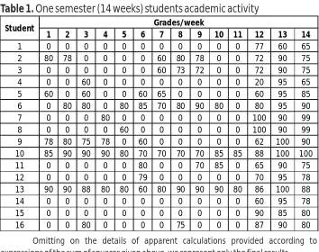
We consider usage of the suggested evaluation procedure with an example of a group of the first year students, who studied English Language during 1 Semester lasting for 14 weeks (International Black see University, Department of American Studies). Total number of evaluated students is 16 (so, m=14 and n=16). The corresponding data are given in the tab.1

j H i H j H i H ij

H

if

s

s

s

s

k

=

1

−

≤

i H j H i H j H ji

H

if

s

s

s

s

k

=

1

−

≤

j S i S j S i S ij

S

if

s

s

s

s

k

=

1

−

≤

i S j S i S j S ji

S

if

s

s

s

s

k

=

1

−

≤

j T i T j T i T ij

T

if

s

s

s

s

k

=

1

−

≤

i T j T i T j T ji

T

if

s

s

s

s

Table 1.

Omitting on the details of apparent calculations provided according to expressions of the sum of squares given above, we represent only the final results.

Sums of squares are as follows: SS =370,788.96; SS =264,165.21; T S

mSS =106,759.75. Corresponding indices' values are: k =0.71 and k =0.29. It means that H H S

the group under consideration can be characterized as academically moderately

homogeneous (k -close to 1) and at the same time, strongly unstable (low values of k ). H S

The last results in quite low value of the group total average grade µ =37.

Table 2. Stability Indices

One semester (14 weeks) students academic activity

Student Grades/week

1 2 3 4 5 6 7 8 9 10 11 12 13 14

1 0 0 0 0 0 0 0 0 0 0 0 77 60 65

2 80 78 0 0 0 0 60 80 78 0 0 72 90 75

3 0 0 0 0 0 0 60 73 72 0 0 72 90 75

4 0 0 60 0 0 0 0 0 0 0 0 20 95 65

5 60 0 60 0 0 60 65 0 0 0 0 60 95 85

6 0 80 80 0 80 85 70 80 90 80 0 80 95 90

7 0 0 0 80 0 0 0 0 0 0 0 100 90 99

8 0 0 0 0 60 0 0 0 0 0 0 100 90 99

9 78 80 75 78 0 60 0 0 0 0 0 62 100 90

10 85 90 90 90 80 70 70 70 70 85 85 88 100 100

11 0 0 0 0 0 80 0 0 70 85 0 65 90 75

12 0 0 0 0 0 79 0 0 0 0 0 70 95 78

13 90 90 88 80 80 60 80 90 90 90 80 86 100 88

14 0 0 0 0 0 0 0 0 0 0 0 60 95 78

15 0 0 0 0 0 0 0 0 0 0 0 90 85 80

16 0 0 80 0 0 0 0 75 0 0 0 87 90 80

Students Average

Grades

2

)

( ij i

M g g

SS _i = −

M M M

SS SS

k i

i = 1 −

1 2 2 3

1 14.43 10,839.43 0.96

2 43.79 20,636.36 0.92

3 31.57 19,067.43 0.93

4 17.14 13,135.71 0.95

5 34.64 18,073.21 0.93

6 65.00 16,600.00 0.94

7 26.36 24,575.21 0.91

8 24.93 22,800.93 0.91

Stability index clarifies the reason why the average grades of students 10 and 13 are incomparably higher than the others: the students are absolutely stable with stability indices 0.99 and 1.

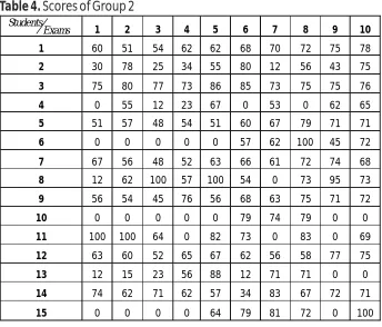
b. Comparison of two groups

Both groups comprise 15 students and 10 tests. Evaluation scale is 100 grades.

4

Grades are shown in tab.3 and 4 . In this case, according to (7),

Table 3. Scores of Group 1

10 83.79 1,438.36 0.99

11 33.21 21,030.36 0.92

12 23.00 18,844.00 0.93

13 85.14 1,093.71 1.00

14 16.64 14,831.21 0.94

15 18.21 17,080.36 0.94

16 29.43 21,969.43 0.92

375000 10

15 2500 2500

max = = ⋅ ⋅ =

mn SST

4

As correct comparison of results of different groups of students needs prior equating [4], data in tab. 3 and 4 have been preliminary equated.

Exams

Students _{1 2 3 4 5 6 7 8 9 10}

1 47 81 70 73 80 79 72 75 77 89

2 88 67 91 96 78 90 83 88 89 93

3 82 74 69 81 76 84 75 83 85 84

4 67 73 75 63 67 79 78 79 93 88

5 90 83 92 92 88 98 85 98 88 94

6 37 56 70 65 72 65 76 78 76 86

7 46 58 75 79 67 78 86 74 81 74

8 48 79 79 64 78 86 94 79 74 69

9 58 62 59 68 80 79 79 86 75 79

10 45 46 71 72 78 73 75 79 75 74

11 56 88 81 66 74 76 73 87 79 78

12 68 78 64 75 79 72 79 79 73 84

13 52 65 79 62 59 67 75 75 83 68

14 38 57 73 85 68 77 75 67 73 56

Table 4.

The results of calculation of basic Mean Sums of Squares and Comparative Indices (the latter are calculated according to (7), (8) and (9) formulas) are shown in tab.5

Table 5. Comparative sums and indices

From the first glance it is difficult to find difference among two sets of scores, but elaborated comparative methodology permits to discover quite significant difference between two groups of students under consideration. The second group has all characteristics better than the first one: total variability is less almost with 30%, heterogeneity -45% and stability – 23%. Clear that it means that teaching process in the second group should be evaluated as more efficient. The latter gives objective basis for final evaluation of teaching review.

Scores of Group 2

Exams Students

1 2 3 4 5 6 7 8 9 10

1 60 51 54 62 62 68 70 72 75 78

2 30 78 25 34 55 80 12 56 43 75

3 75 80 77 73 86 85 73 75 75 76

4 0 55 12 23 67 0 53 0 62 65

5 51 57 48 54 51 60 67 79 71 71

6 0 0 0 0 0 57 62 100 45 72

7 67 56 48 52 63 66 61 72 74 68

8 12 62 100 57 100 54 0 73 95 73

9 56 54 45 76 56 68 63 75 71 72

10 0 0 0 0 0 79 74 79 0 0

11 100 100 64 0 82 73 0 83 0 69

12 63 60 52 65 67 62 56 58 77 75

13 12 15 23 56 88 12 71 71 0 0

14 74 62 71 62 57 34 83 67 72 71

15 0 0 0 0 64 79 81 72 0 100

Sum of Squares (Group 1)

Sum of Squares (Group 2)

Comparative Indices

MSST=134.72 MSST=94.48

k

=

29

.

87

%

MSSS=103.10 MSSS=24.07

45

.

26

%

21

₌

H

k

6. Conclusion

A new method of quantitative evaluation for teaching processes review is elaborated. On the base of scores data, the method permits to evaluate efficiency of teaching within one group of students and comparative teaching efficiency in two or more groups. As basic characteristics of teaching efficiency heterogeneity, stability and total variability indices both for only one group and for comparing different groups are introduced. The method is easy to use and permits to rank results of teaching review which is the one of the most important parts of general quality control in education.

References

El-Khawas, E. (1998). Accreditation’s role in Quality Assurance in the United States. Higher Education Management, 10

Harvey, L., Green, D. (1993). Defining Quality. Assessment and Evaluation in Higher Education,18.

Harvey, L. (1999). An Assessment of Past and Current Approaches to Quality in Higher Education. Australian Journal of Education, 43(3).

Milnikova I. (2011). Basic Conceptions of statistical quality control in education. Scientific Journal of International Black Sea University, 5(2): 83-92.