E
E
F
F
F
F
I
I
C
C
I
I
E
E
N
N
C
C
Y
Y
O
O
F
F
D
D
A
A
T
T
A
A
T
T
R
R
A
A
N
N
S
S
F
F
O
O
R
R
M
M
A
A
T
T
I
I
O
O
N
N
A
A
N
N
D
D
C
C
O
O
R
R
R
R
E
E
C
C
T
T
I
I
O
O
N
N
F
F
A
A
C
C
T
T
O
O
R
R
M
M
E
E
T
T
H
H
O
O
D
D
S
S
O
O
N
N
T
T
H
H
E
E
C
C
O
O
R
R
R
R
E
E
C
C
T
T
I
I
O
O
N
N
O
O
F
F
E
E
X
X
T
T
R
R
E
E
M
M
E
E
V
V
A
A
L
L
U
U
E
E
E
E
F
F
F
F
E
E
C
C
T
T
I
I
N
N
S
S
A
A
M
M
P
P
L
L
E
E
S
S
U
U
R
R
V
V
E
E
Y
Y
T
T
H
H
E
E
O
O
R
R
Y
Y
P
P
e
e
t
t
e
e
r
r
I
I
.
.
O
O
g
g
u
u
n
n
y
y
i
i
n
n
k
k
a
a
11,
,
E
E
m
m
m
m
a
a
n
n
u
u
e
e
l
l
F
F
.
.
O
O
l
l
o
o
g
g
u
u
n
n
l
l
e
e
k
k
o
o
22,
,
B
B
.
.
T
T
.
.
E
E
f
f
u
u
w
w
a
a
p
p
e
e
11,
,
O
O
.
.
M
M
.
.
O
O
l
l
a
a
y
y
i
i
w
w
o
o
l
l
a
a
33,
,
D
D
a
a
w
w
u
u
d
d
A
A
.
.
A
A
g
g
u
u
n
n
b
b
i
i
a
a
d
d
e
e
111 Department of Mathematical Sciences, Olabisi Onabanjo University, Ago-Iwoye, Nigeria 2 Department of Statistics, University of Ibadan, Ibadan, Nigeria
3 Department of Statistics, Federal University of Agriculture, Abeokuta, Nigeria
Corresponding Author: Peter I. Ogunyinka, [email protected] ABSTRACT: Extreme value, in Sample Survey Theory, is
termed outlier in General Statistical Theory. Extreme value data analysis would yield over-estimation or under-estimation in statistical under-estimation process. Non-linear data transformation method and Sarndal’s correction factor method in Sample Survey Theory have been confirmed to correct extreme value effect in an estimate. However, since the two methods work towards the same objective, there is need to ascertain the efficient estimate between the two methods. This study has empirically compared the two extreme value correction methods. Results revealed that non-linear data transformation method, though associated with back transformation challenge, had lower Percentage Coefficient of Variation (PCV) over correction factor method. Hence, non-linear data transformation method proved efficient over correction factor method. It was recommended that Survey Statisticians should improve on the Sarndal’s developed correction factor method and/or developed new improved estimators for the correction of extreme value in Sample Survey Theory.
KEYWORDS: Extreme value, non-linear data transformation, correction factor, regression estimator, percentage coefficient of variation.
1.
INTRODUCTIONThe Survey Statisticians leverage on the presence of auxiliary information in any data set to improve on any concerned estimators. Single-phase sampling estimator like ratio ([Coc40)], regression ([Coc42]), product ([HHM53]) and difference ([Rob57]) estimators and two-phase sampling estimators ([Ney38] and [Kee05]) have used auxiliary information (either auxiliary variable or attribute) to produce different Uniformly Minimum Variance (UMV) estimators in Sample Survey Theory. The use of single-phase sampling requires positive and high correlation coefficient between the study variable (𝑦) and the auxiliary variable (𝑥) ([AO13]). Among the statistical assumptions required for the use of single-phase sampling estimator are linearity assumption between the study and the auxiliary
variable and the normality assumption. However, the violation of these assumptions will lead to over-estimation or under-over-estimation of the concerned parameter ([Sar72]), therefore, increasing the Mean Square Error (MSE) of the estimate. The presence of extreme value in a data set has been confirmed as the major source of the violation of statistical assumption ([A+18]).
Extreme value in Sample Survey Theory is also called outlier in General Statistics Theory. Extreme value could be identified in the data set as outrageously high observation(s) or outrageously low observation(s) in the data set. The prior detection of the presence of extreme value in the data set, to the application of estimators, is very germane to obtaining efficient estimate. Ratio, regression, difference and product estimators are also affected by the presence of extreme value in the data set which produce less efficient estimate. This study has identified two solutions for the correction of extreme value(s) in the data set. The use of non-linear data transformation on the data set prior to the estimation of the parameter and the use of correction factor in the estimator ([Sar72]) are the solutions considered in this study.
2. METHODOLOGY
2.1 The theory of data transformation and Sarndal’s correction factor
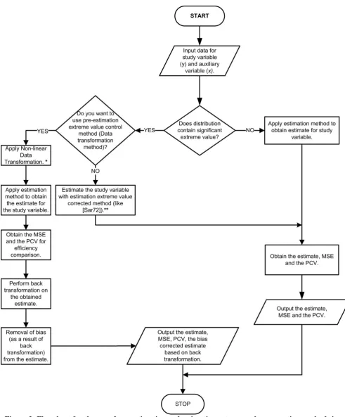
been ascertained by [TF07], some authors have reported the set-back or challenge of back transformation to be associated with non-linear data transformation. [OB14] has applied non-linear data transformation to the estimation of online software repository variables. Table 1 shows the varieties of non-linear transformation tools used by [OB14]. Those tools include exponential, quadratic, reciprocal, logarithm, power and square transformations. Back transformation is a major challenge associated with non-linear data transformation. Fortunately, while it cannot be avoided, it can be minimized. [Mil84] and [JR08] are among the major theoretical back transformation solutions that are recognized by authors to have reduced the bias introduced by back transformation. This study has classified data transformation as a pre-estimation extreme value control method since it is applied prior to the estimation of the parameter. [Sar72] had developed an improved estimator using optimum correction factor (𝐶𝑜𝑝𝑡) to minimize the effect of extreme value within the data set. Sarndal assumed that this correction factor (𝐶𝑜𝑝𝑡) should be added to the estimator if the extreme value causes under-estimation but subtracted if the extreme value causes over-estimation. This study has classified Sarndal’s correction factor method as estimation extreme value correction method since the correction factor is embedded in the estimator. Figure 2 shows the flowchart on the procedural application of data transformation and control factor methods. It also explains the pre-estimation and estimation extreme value correction methods. The flowchart illustration on the use of pre-estimation (non-linear data transformation) is also applicable to General Statistical Theory.
In a data set with 𝑦 as the unbiased estimator of the population mean, 𝑦𝑚𝑖𝑛 as the minimum extreme value and 𝑦𝑚𝑎𝑥 as the maximum extreme value, [Sar72] has suggested an efficient sample mean with the correction factor (𝐶𝑜𝑝𝑡) as
𝑦𝑠 = {
𝑦 + 𝑐 𝑖𝑓 𝑠𝑎𝑚𝑝𝑙𝑒 𝑐𝑜𝑛𝑡𝑎𝑖𝑛𝑠 𝑦𝑚𝑖𝑛 𝑜𝑛𝑙𝑦
𝑦 − 𝑐 𝑖𝑓 𝑠𝑎𝑚𝑝𝑙𝑒 𝑐𝑜𝑛𝑡𝑎𝑖𝑛𝑠 𝑦𝑚𝑎𝑥 𝑜𝑛𝑙𝑦
𝑦 𝑓𝑜𝑟 𝑎𝑙𝑙 𝑜𝑡ℎ𝑒𝑟 𝑠𝑎𝑚𝑝𝑙𝑒𝑠,
(1)
where 0 < 𝑐 < (𝑦𝑚𝑎𝑥− 𝑦𝑚𝑖𝑛) 𝑛⁄ and 𝑛 is the sample size.
The optimum value of 𝑐 is presented as 𝑐𝑜𝑝𝑡= (𝑦𝑚𝑎𝑥−𝑦𝑚𝑖𝑛)
2𝑛 and the optimum variance of 𝑦𝑠 is presented as
𝑉(𝑦𝑠)
𝑚𝑖𝑛= 𝑉(𝑦) −
𝜃∆𝑦2
2(𝑁−1). (2)
where 𝑉(𝑦) = 𝜃𝑆𝑦2, ∆𝑦= (𝑦𝑚𝑎𝑥− 𝑦𝑚𝑖𝑛), 𝜃 =
(𝑛1−𝑁1), 𝑁 = population size and 𝑛 = Sample size. [Coc42] developed regression estimator of the study variable (𝑦) in relationship with the auxiliary variable (𝑥) as
𝑦𝑙𝑟= 𝑦 + 𝑏(𝑋 − 𝑥). (3)
The corresponding minimized variance of 𝑦𝑙𝑟 is presented as:
𝑉(𝑦𝑙𝑟)
𝑚𝑖𝑛 = 𝜃𝑆𝑦
2(1 − 𝜌
𝑦𝑥2 ), (4)
where 𝜌𝑦𝑥 = Correlation coefficient.
[KS13] seems to be the first to improve regression estimators for estimating the population mean in the presence of extreme value in the data set using the correction factor of [Sar72]. The improved estimators is presented as
𝑦𝑙𝑟𝑐=
{
(𝑦 + 𝑐1) + 𝑏 (𝑋 − (𝑥 + 𝑐2)) , 𝑖𝑓 𝑠𝑎𝑚𝑝𝑙𝑒
𝑐𝑜𝑛𝑡𝑎𝑖𝑛𝑠 𝑦𝑚𝑖𝑛 𝑜𝑛𝑙𝑦;
(𝑦 − 𝑐1) + 𝑏 (𝑋 − (𝑥 − 𝑐2)) , 𝑖𝑓 𝑠𝑎𝑚𝑝𝑙𝑒
𝑐𝑜𝑛𝑡𝑎𝑖𝑛𝑠 𝑦𝑚𝑎𝑥 𝑜𝑛𝑙𝑦
𝑦 + 𝑏(𝑋 − 𝑥), 𝑓𝑜𝑟 𝑎𝑙𝑙 𝑜𝑡ℎ𝑒𝑟 𝑠𝑎𝑚𝑝𝑙𝑒𝑠.
(5)
The corresponding variance is presented as
𝑉(𝑦𝑙𝑟𝑐) = 𝑉(𝑦𝑙𝑟) −(𝑁−1)2𝜃𝑛 [(𝑐1− 𝛽𝑐2){∆𝑦− 𝛽∆𝑥−
2𝑛(𝑐1− 𝛽𝑐2)}]. (6)
The optimum values of 𝑐1 and 𝑐2 are presented as
𝑐1𝑜𝑝𝑡 =(𝑦𝑚𝑎𝑥
−𝑦𝑚𝑖𝑛)
2𝑛 and 𝑐2𝑜𝑝𝑡 =
(𝑥𝑚𝑎𝑥−𝑥𝑚𝑖𝑛) 2𝑛 . The minimized variance is presented as
𝑉(𝑦𝑙𝑟𝑐)
𝑚𝑖𝑛= 𝑉(𝑦𝑙𝑟) −
𝜃
2(𝑁−1)[∆𝑦− 𝛽∆𝑥] 2
, (7)
where ∆𝑦= (𝑦𝑚𝑎𝑥− 𝑦𝑚𝑖𝑛), ∆𝑥= (𝑥𝑚𝑎𝑥− 𝑥𝑚𝑖𝑛) and 𝛽 is the regression coefficient of 𝑦 on 𝑥.
theoretically unlike Sarndal’s correction method. Therefore, this study shall examine the efficiency of these two correction methods empirically.
Table 1 shows different transformation tools that will lead to different units of measurement of the study variable and the variance. Consequently, all
the estimates and variances that will be compared will be in different units of measurement. Hence, there is need for a statistical measure that can be used for comparison in this case. The Coefficient of Variation (CV) will be a better choice.
Table 1: Some of the mathematical tools used in non-linear data transformation (extracted from [OB14])
SN Dependent
Variable (𝑇)
Independent
Variable (𝐷) Linear Regression Model
Back Transformation
1 𝑇 𝑙𝑜𝑔10𝐷 = 𝐷∗ 𝑇 = 𝛼 + 𝛽𝐷∗ 𝑇̂ = 𝛼 + 𝛽𝐷∗
2 𝑙𝑜𝑔10𝐷 = 𝐷∗ 3√𝑇= 𝑇∗ 𝐷∗= 𝛼 + 𝛽𝑇∗ 𝐷̂ = 10(𝛼+𝛽𝑇
∗)
3 𝑙𝑜𝑔10𝑇 = 𝑇∗ 𝑙𝑜𝑔10𝐷 = 𝐷∗ 𝑇∗= 𝛼 + 𝛽𝐷∗ 𝑇̂ = 10(𝛼+𝛽𝐷
∗)
4 √𝐷 = 𝐷∗ √𝑇3 = 𝑇∗ 𝐷∗= 𝛼 + 𝛽𝑇∗ 𝐷̂ = (𝛼 + 𝛽𝑇∗)2
5 𝑙𝑜𝑔2𝑇 = 𝑇∗ 𝑙𝑜𝑔10𝐷 = 𝐷∗ 𝑇∗= 𝛼 + 𝛽𝐷∗ 𝑇̂ = 2(𝛼+𝛽𝐷
∗)
6 √𝐷 = 𝐷∗ 𝑇2= 𝑇∗ 𝐷∗= 𝛼 + 𝛽𝑇∗ 𝐷̂ = (𝛼 + 𝛽𝑇∗)2
7 𝑇 √𝐷 = 𝐷∗ 𝑇 = 𝛼 + 𝛽𝐷∗ 𝑇̂ = 𝛼 + 𝛽𝐷∗
8 √𝑇 = 𝑇∗ √𝐷 = 𝐷∗ 𝑇∗= 𝛼 + 𝛽𝐷∗ 𝑇̂ = (𝛼 + 𝛽𝐷∗)2
9 𝑙𝑜𝑔10𝑇 = 𝑇∗ 𝐷−1= 𝐷∗ 𝑇∗= 𝛼 + 𝛽𝐷∗ 𝑇̂ = 10(𝛼+𝛽𝐷
∗)
10 𝑇3= 𝑇∗ 𝐷 𝑇∗= 𝛼 + 𝛽𝐷 𝑇̂ = √(𝛼 + 𝛽𝐷)3
11 𝐷 𝑇2= 𝑇∗ 𝐷 = 𝛼 + 𝛽𝑇∗ 𝐷̂ = 𝛼 + 𝛽𝑇∗
12 𝑇3= 𝑇∗ √𝐷3 = 𝐷∗ 𝑇∗= 𝛼 + 𝛽𝐷∗ 𝑇̂ = √(𝛼 + 𝛽𝐷3 ∗)
13 𝑙𝑜𝑔10𝐷 = 𝐷∗ 𝑇−1= 𝑇∗ 𝐷∗= 𝛼 + 𝛽𝑇∗ 𝐷̂ = 10(𝛼+𝛽𝑇
∗)
14 𝑇−1= 𝑇∗ 𝐷−1= 𝐷∗ 𝑇∗= 𝛼 + 𝛽𝐷∗ 𝑇̂ = (𝛼 + 𝛽𝐷∗)−1
Coefficient of Variation (CV) is a statistical measure of variability for any experiment with different units of measurement. The CV has the major advantage because it converts experiment to a dimensionless output. Hence, it makes the comparison of experiment with different measurement of unit possible. [Man13] reported that [CCK67] developed coefficient of variation while [M+017] reported on the classification of CV. However, this study will not be concerned with the classification of CV. The lower the CV, the more efficient is the concerned estimate or estimator. The higher the CV, the least efficient is the concerned estimate or estimator. The Percentage Coefficient of Variation (PCV) is presented as
𝑃𝐶𝑉 = 𝑆𝐸
𝑀𝑒𝑎𝑛∗ 100%, (8)
where 𝑆𝐸= Standard error.
3. RESULTS AND DISCUSSION 3.1 Results
Table 2 explains the classification of correlation coefficient based on the recommendations of [AO13]. M represents Moderate correlation coefficient and H represents High correlation coefficient. Tables 3 through 7 show analysis results
for different population sizes (𝑁) and sample sizes
(𝑛). Table 3 has 𝑁 = 150 and 𝑛 = 30, table 4 has
𝑁 = 200 and 𝑛 = 30, table 5 has 𝑁 = 200 and 𝑛 =
50, table 6 has 𝑁 = 250 and 𝑛 = 70 and table 7 has
𝑁 = 250 and 𝑛 = 90. Analysis in table 3 through 7
shows the results of the correlation coefficient, the classification of the correlation coefficient, the confirmation of the outlier in the data set, confirmation of the violation of linearity assumption (represented in A1), independence assumption (represented in A2), normality assumption (represented in A3) and homoscedasticity assumption (represented in A4).
Table 2: Correlation Coefficient interpretation extracted from [AO13]
Size range of Correlation
Interpretation Notation
0.90 to 1.0 Very high Positive (Negative) Correlation
V 0.70 to <0.90 High Positive (Negative)
Correlation
H 0.50 to <0.70 Moderate Positive
(Negative) Correlation
M 0.30 to <0.50 Low Positive (Negative)
Correlation
They also show the population mean estimates obtained after applying non-linear data transformation and using correction factor in [KS13] regression estimator. Finally, the corresponding variance, Percentage Coefficient of Variation (PCV) and the rank of the PCV were presented in the five tables. The analyses measure the rank of correlation coefficient, confirmed the presence of outlier and the violation of statistical assumptions. The ranking results (in the last column of tables 3 through 7) ranked the correction method and estimators based on results of the PCV in ascending order since lower PCV signifies higher efficiency of the estimates or estimator and vice versa.
3.2 Discussion
In table 3, the outlier column confirms that the original data contains significant outlier, violated linearity, normality and homoscedasticity assumptions. However, it was, further, revealed that non-linear data transformation on both the study and auxiliary variables corrected the effects of outliers and the violation of statistical assumptions. This justifies the importance of data transformation to the correction of violation of statistical assumptions. [KS13] regression estimator used the original data for analysis. The ranking result (last column in the table) rated the estimate obtained from the original data analysis to be the least (8th with PCV of 11.389%). It was confirmed that estimates obtained from non-linearly transformed data analyses proved efficient (with 1st to 6th ranking of the PCV) over the estimate from the original data. This ascertained the importance of data transformation method in the correction of extreme value in the data set. Estimate from Khan and Shabbir ([KS13]) regression estimator was ranked efficient (7th with PCV of 11.037%) over estimate from the original data analysis (8th with PCV of 11.389%). This shows that Sarndal’s correction factor controls the extreme value effect. Contrarily, Khan and Shabbir ([KS13]) regression estimate proved least efficient (7th with PCV of 11.037%) over the estimates from the non-linear data transformation analysis (with 1st to 6th PCV ranking). This means that the extreme value effect (variability) control of [Sar72] correction
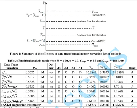
method was not efficient compared to non-linear data transformation extreme value effect control method. Analysis results in tables 4 through 7 confirmed the above emphased results. Hence, it was confirmed that pre-estimation extreme value correction (non-linear data transformation) method proved efficient in correcting the violation of statistical assumptions in the original data. It was also confirmed that non-linear data transformation proved efficient over the use of correction factor in the [KS13] regression estimator. The summary of this discovery is presented in figure 1.
In figure 1, 𝑌 is the parameter to be estimated. The over-estimated and under-estimated estimators,
Figure 1: Summary of the efficiency of data transformation over correction factor methods
Table 3: Empirical analysis result when 𝑵 = 𝟏𝟓𝟎, 𝒏 = 𝟑𝟎, 𝑪𝟏𝒐𝒑𝒕= 𝟎. 𝟖𝟖 and 𝑪𝟐𝒐𝒑𝒕= 𝟒𝟖𝟔𝟕. 𝟎𝟎
SN
Data
Trans-formation 𝝆𝒚𝒙
Out-
lier 𝑨𝟏 𝑨𝟐 𝑨𝟑 𝑨𝟒 𝑦𝑙𝑟 𝑉(𝑦𝑙𝑟) 𝐶𝑉(𝑦𝑙𝑟) Rank
1 𝒚 𝒙⁄ 0.5625 :M yes D O D D 16.1843 3.3973 11.389% 8
2 𝟑√𝒚⁄√𝒙 0.5812 :M no O O O O 2.3671 0.0082 3.818% 3
3 𝟑√𝒚⁄𝟑√𝒙 0.5828 :M no O O O O 2.3774 0.0081 3.796% 2
4 𝟑√𝒚⁄𝒍𝒐𝒈𝟏𝟎𝒙 0.5732 :M no O O O O 2.4002 0.0083 3.791% 1 5 𝒍𝒐𝒈𝟏𝟎𝒚 √𝒙⁄ 0.5580 :M no O O O O 2.5741 0.0116 4.186% 6 6 𝒍𝒐𝒈𝟏𝟎𝒚 √𝒙⁄𝟑 0.5586 :M no O O O O 2.5856 0.0116 4.165% 5
7 𝒍𝒐𝒈𝟏𝟎𝒚 𝒍𝒐𝒈⁄ 𝟏𝟎𝒙 0.5468 :M no O O O O 2.6110 0.0118 4.164% 4
8 [KS13] Regression Estimator 16.5777 3.3475 11.037% 7
Keys: A1 = Linearity assumption; A2 = Independence assumption; A3 = Normality assumption, 𝐴4 = Homoscedasticity assumption, O= Obey assumption, D= Disobey assumption, H= High Correlation Coefficient and M= Medium Correlation Coefficient
Table 4: Empirical analysis result when𝑵 = 𝟐𝟎𝟎, 𝒏 = 𝟑𝟎, 𝑪𝟏𝒐𝒑𝒕= 𝟎. 𝟖𝟓 and 𝑪𝟐𝒐𝒑𝒕= 𝟕𝟏𝟑𝟔. 𝟔
SN
Data
Trans-formation 𝝆𝒚𝒙
Out-
lier 𝑨𝟏 𝑨𝟐 𝑨𝟑 𝑨𝟒 𝑦𝑙𝑟 𝑉(𝑦𝑙𝑟) 𝐶𝑉(𝑦𝑙𝑟) Rank
1 𝒚 𝒙⁄ 0.6895 :M yes D O D D 18.0741 4.4840 11.716% 14
2 𝒚 √𝒙⁄ 0.7575 :H yes O O D O 17.7489 3.6428 10.753% 12
3 𝒚 √𝒙⁄𝟑 0.7713 :H yes O O D O 17.8234 3.4629 10.441% 11
4 𝒚 𝒍𝒐𝒈⁄ 𝟏𝟎𝒙 0.7742 :H yes O O D O 18.2639 3.4239 10.131% 10
5 √𝒚 √𝒙⁄ 0.7277 :H no O O O O 3.7904 0.0500 5.899% 9
6 √𝒚 √𝒙⁄𝟑 0.7447 :H no O O O O 3.7976 0.0473 5.728% 8
7 √𝒚 𝒍𝒐𝒈⁄ 𝟏𝟎𝒙 0.7547 :H no O O O O 3.8441 0.0457 5.563% 7
8 𝟑√𝒚⁄√𝒙 0.7105 :H no O O O O 2.3700 0.0091 4.035% 3
9 𝟑√𝒚⁄𝟑√𝒙 0.7281 :H no O O O O 2.3729 0.0087 3.925% 2
10 𝟑√𝒚⁄𝒍𝒐𝒈𝟏𝟎𝒙 0.7397 :H no O O O O 2.3917 0.0084 3.823% 1 11 𝒍𝒐𝒈𝟏𝟎𝒚 √𝒙⁄ 0.6779 :M no O O O O 2.5535 0.0127 4.410% 6 12 𝒍𝒐𝒈𝟏𝟎𝒚 √𝒙⁄𝟑 0.6962 :M no O O O O 2.5565 0.0121 4.302% 5
13 𝒍𝒐𝒈𝟏𝟎𝒚 𝒍𝒐𝒈⁄ 𝟏𝟎𝒙 0.7100 :H no O O O O 2.5766 0.0116 4.187% 4
14 [KS13] Regression Estimator 18.0851 4.4218 11.627% 13
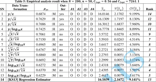
Table 5: Empirical analysis result when 𝑵 = 𝟐𝟎𝟎, 𝒏 = 𝟓𝟎, 𝑪𝟏𝒐𝒑𝒕= 𝟎. 𝟓𝟔 and 𝑪𝟐𝒐𝒑𝒕= 𝟕𝟐𝟔𝟏. 𝟏
SN
Data
Trans-formation 𝝆𝒚𝒙
Out-
lier 𝑨𝟏 𝑨𝟐 𝑨𝟑 𝑨𝟒 𝑦𝑙𝑟 𝑉(𝑦𝑙𝑟) 𝐶𝑉(𝑦𝑙𝑟) Rank
1 𝒚 𝒙⁄ 0.6874 :M yes D O D D 16.0146 2.1702 9.199% 14
2 𝒚 √𝒙⁄ 0.7629 :H yes O O D D 16.1309 1.7197 8.130% 12
3 𝒚 √𝒙⁄𝟑 0.7686 :H yes O O D D 16.3012 1.6837 7.960% 10
4 𝒚 𝒍𝒐𝒈⁄ 𝟏𝟎𝒙 0.7425 :H yes O O D D 16.7778 1.8465 8.099% 11
5 √𝒚 √𝒙⁄ 0.7061 :H no O O D O 3.5732 0.0270 4.595% 9
6 √𝒚 √𝒙⁄𝟑 0.7150 :H no O O D O 3.5910 0.0263 4.514% 7
7 √𝒚 𝒍𝒐𝒈⁄ 𝟏𝟎𝒙 0.6965 :M no O O D O 3.6417 0.0277 4.569% 8
8 𝟑√𝒚⁄√𝒙 0.6767 :M no O O O O 2.2721 0.0052 3.184% 3
9 𝟑√𝒚⁄√𝒙𝟑 0.6860 :M no O O O O 2.2793 0.0051 3.136% 1
10 𝟑√𝒚⁄𝒍𝒐𝒈𝟏𝟎𝒙 0.6692 :M no O O O O 2.2999 0.0053 3.174% 2 11 𝒍𝒐𝒈𝟏𝟎𝒚 √𝒙⁄ 0.6272 :M no O O O O 2.4318 0.0079 3.646% 6 12 𝒍𝒐𝒈𝟏𝟎𝒚 √𝒙⁄𝟑 0.6370 :M no O O O O 2.4395 0.0077 3.597% 4
13 𝒍𝒐𝒈𝟏𝟎𝒚 𝒍𝒐𝒈⁄ 𝟏𝟎𝒙 0.6229 :M no O O O O 2.4617 0.0079 3.617% 5
14 [KS13] Regression Estimator 16.1039 2.1672 9.141% 13
Keys: A1 = Linearity assumption; A2 = Independence assumption; A3 = Normality assumption, 𝐴4 = Homoscedasticity assumption, O= Obey assumption, D= Disobey assumption, H= High Correlation Coefficient and M= Medium Correlation Coefficient.
Table 6: Empirical analysis result when 𝑵 = 𝟐𝟓𝟎, 𝒏 = 𝟕𝟎, 𝑪𝟏𝒐𝒑𝒕= 𝟎. 𝟓𝟗𝟐𝟗 and 𝑪𝟐𝒐𝒑𝒕= 𝟕𝟎𝟔𝟗. 𝟓𝟑
SN
Data
Trans-formation 𝝆𝒚𝒙
Out-
lier 𝑨𝟏 𝑨𝟐 𝑨𝟑 𝑨𝟒 𝑦𝑙𝑟 𝑉(𝑦𝑙𝑟) 𝐶𝑉(𝑦𝑙𝑟) Rank
1 𝒚 𝒙⁄ 0.6163 :M yes D O D D 16.5025 2.6005 9.772% 14
2 𝒚 √𝒙⁄ 0.7612 :H yes O O D D 17.4438 1.7638 7.613% 12
3 𝒚 √𝒙⁄𝟑 0.7872 :H yes O O D D 17.2777 1.5950 7.310% 11
4 𝒚 𝒍𝒐𝒈⁄ 𝟏𝟎𝒙 0.7665 :H yes O O D D 18.1679 1.7293 7.238% 10
5 √𝒚 √𝒙⁄ 0.7455 :H no O O D O 3.6032 0.0193 3.853% 9
6 √𝒚 √𝒙⁄𝟑 0.7753 :H no O O D O 3.6398 0.0173 3.614% 8
7 √𝒚 𝒍𝒐𝒈⁄ 𝟏𝟎𝒙 0.7689 :H no O O D O 3.7298 0.0177 3.571% 7
8 𝟑√𝒚⁄√𝒙 0.7234 :H no O O D O 2.2787 0.0035 2.610% 3
9 𝟑√𝒚⁄√𝒙𝟑 0.7544 :H no O O D O 2.2934 0.0032 2.465% 2
10 𝟑√𝒚⁄𝒍𝒐𝒈𝟏𝟎𝒙 0.7542 :H no O O D O 2.3297 0.0032 2.428% 1 11 𝒍𝒐𝒈𝟏𝟎𝒚 √𝒙⁄ 0.6763 :M no O O O D 2.4319 0.0051 2.944% 6 12 𝒍𝒐𝒈𝟏𝟎𝒚 √𝒙⁄𝟑 0.7087 :H no O O O D 2.4473 0.0047 2.802% 5
13 𝒍𝒐𝒈𝟏𝟎𝒚 𝒍𝒐𝒈⁄ 𝟏𝟎𝒙 0.7182 :H no O O O O 2.4860 0.0046 2.721% 4
14 [KS13] Regression Estimator 16.5960 2.5969 9.710% 13
Keys: A1 = Linearity assumption; A2 = Independence assumption; A3 = Normality assumption, 𝐴4 = Homoscedasticity
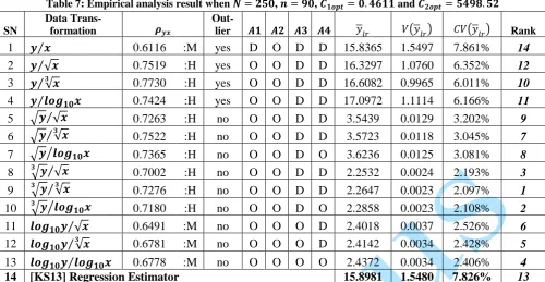
Table 7: Empirical analysis result when 𝑵 = 𝟐𝟓𝟎, 𝒏 = 𝟗𝟎, 𝑪𝟏𝒐𝒑𝒕= 𝟎. 𝟒𝟔𝟏𝟏 and 𝑪𝟐𝒐𝒑𝒕= 𝟓𝟒𝟗𝟖. 𝟓𝟐
SN
Data
Trans-formation 𝝆𝒚𝒙
Out-
lier 𝑨𝟏 𝑨𝟐 𝑨𝟑 𝑨𝟒 𝑦𝑙𝑟 𝑉(𝑦𝑙𝑟) 𝐶𝑉(𝑦𝑙𝑟) Rank
1 𝒚 𝒙⁄ 0.6116 :M yes D O D D 15.8365 1.5497 7.861% 14
2 𝒚 √𝒙⁄ 0.7519 :H yes O O D D 16.3297 1.0760 6.352% 12
3 𝒚 √𝒙⁄𝟑 0.7730 :H yes O O D D 16.6082 0.9965 6.011% 10
4 𝒚 𝒍𝒐𝒈⁄ 𝟏𝟎𝒙 0.7424 :H yes O O D D 17.0972 1.1114 6.166% 11
5 √𝒚 √𝒙⁄ 0.7263 :H no O O D D 3.5439 0.0129 3.202% 9
6 √𝒚 √𝒙⁄𝟑 0.7522 :H no O O D D 3.5723 0.0118 3.045% 7
7 √𝒚 𝒍𝒐𝒈⁄ 𝟏𝟎𝒙 0.7365 :H no O O D O 3.6236 0.0125 3.081% 8
8 𝟑√𝒚⁄√𝒙 0.7002 :H no O O D D 2.2532 0.0024 2.193% 3
9 𝟑√𝒚⁄√𝒙𝟑 0.7276 :H no O O D D 2.2647 0.0023 2.097% 1
10 𝟑√𝒚⁄𝒍𝒐𝒈𝟏𝟎𝒙 0.7180 :H no O O D O 2.2858 0.0023 2.108% 2 11 𝒍𝒐𝒈𝟏𝟎𝒚 √𝒙⁄ 0.6491 :M no O O O D 2.4018 0.0037 2.526% 6 12 𝒍𝒐𝒈𝟏𝟎𝒚 √𝒙⁄𝟑 0.6781 :M no O O O D 2.4142 0.0034 2.428% 5
13 𝒍𝒐𝒈𝟏𝟎𝒚 𝒍𝒐𝒈⁄ 𝟏𝟎𝒙 0.6778 :M no O O O O 2.4372 0.0034 2.406% 4
14 [KS13] Regression Estimator 15.8981 1.5480 7.826% 13
Keys: A1 = Linearity assumption; A2 = Independence assumption; A3 = Normality assumption, 𝐴4 = Homoscedasticity assumption, O= Obey assumption, D= Disobey assumption, H= High Correlation Coefficient and M= Medium Correlation Coefficient.
4. CONCLUSIONS
Attention had been called to the sequency of extreme value and outlier in both Sample Survey Theory and General Statistical Theory, respectively. The presence of extreme value in a data set would cause over-estimation or under-over-estimation which consequently increases the Mean Square Error of the estimate. This study has considered non-linear data transformation and [Sar72] correction factor for the reduction or removal of extreme value effect in Sample Survey Theory. Non-linear data transformation was classified as a pre-estimation extreme value control method and [Sar72] correction factor was defined as an estimation extreme value control method in Sample Survey Theory. This study has compared the efficiency of these two methods using in-depth empirical approach. It was discovered that while non-linear data transformation method is associated with back transformation challenge, estimates from non-linearly transformed data set would significantly reduce the effect of extreme value than estimators with [Sar72] correction factor method. It was empirically ascertained that non-linear data transformation method will produce efficient estimates over [Sar72] correction factor method but not without its associated back transformation bias challenge. Consequently, this study has recommended improvement on the [Sar72] extreme value effect correction method and/or the need to develop another improved estimation extreme value correction method in Sample Survey Theory.
REFERENCES
[AO13] D. A. Agunbiade, P. I. Ogunyinka – Effect of correlation level on the use of Auxiliary variable in Double sampling for regression estimation, Open Journal
of Statistics, Doi:
http//dx.doi.org/10.4236/ojs.2013.3503 7, 2013.
[A+18] N. Abbas, M. Abid, Tahir, M., Abbas, Z. Hussain – Enhancing ratio estimators for estimating population mean using maximum value of auxiliary variable, J. Natn. Sci. Foundation Sri Lanka, vol. 46(3): 453-463, 2018. [Coc40] W. G. Cochran – Sampling Technique,
3rd Edition, Wiley Eastern Limited, India, 1940.
[Coc42] W. G. Cochran – Sampling theory when the sampling units are of unequal sizes, J.Amer. Statistics Association, Vol. 37: 199-212, 1942.
Figure 2: Flowchart for the use of pre-estimation and estimation extreme value correction methods in Sample Survey Theory
Notes to Figure 2.0
* Non-linear data transformation is applied prior to the estimation of the parameters. This is termed pre-estimation extreme value correction method.
** Extreme value correction is coming at the estimation stage. This is termed as estimation extreme value correction method.
[HHM53] M. H. Hansen, W. N. Hurwitz, W. G. Madow – Sample Survey Methods and Theory, 2nd, Ed., New York: Wiley and Sons, 1953.
[JR08] S. Jai, S. Rathi – On predicting log-transformed linear models with heteroscedaticity, SAS Global Forum, Paper 370, 2008.
[Kee05] K. J. Keen – Two Phase Sampling. Encyclopedia of Bio-Statstics, 8, 1-4, 2005.
[KS13] M. Khan, J. Shabbir – Some improved ratio, product and regression estimators of finite population mean when using minimum and maximum values, The Scientific World Journal, Article ID: 431868, 1-7, 2013.
[Man13] M. Manuel – A Coefficient of variability, Journal of Mathematics and Statistics, vol. 9(11), 62-64, ISSN:
1549-3644, dou:
10.3844/jmssp.2013.62.64, 2013. [Mil84] D. Miller – Reducing transformation
bias in Curve fitting, The American Statistician, 30(2), 124-126, 1984. [M+17] A. B. V. Marcos, P. S. Pacheco, E. J.
Seidel, P. A. Angela – Classification of the coefficient of variation to variables in beef Cattle experiments. Ciencia Rural, Santa Maria, vol. 47(1), 1-4,
http://dx.doi.org/10.1590/0103-8478cr20160946, ISSNe: 1678-4596, 2017.
[Ney38] J. Neyman – Contribution to the theory of sampling human populations. J. Amer. Statist. Assoc., Vol. 33, 101-116, 1938.
[OB14] P. I. Ogunyinka, I. Badmus – Efficient linearity of online software repository variables. 5th Series of Proceedings. International Conference on science, Technology, Education, Arts, Management and Social Sciences. Isteams Research Nexus Conference, Afe Babalola University, Ado-Ekiti, Nigeria. Pp. 453-458, 2014.
[Rob57] D. Robson – Application of Multivariate Polykays to the Theory of unbiase Ratio Type Estimators. Journal of American Statistical Association 52: 511-522, 1957.
[Sar72] C. Sarndal – Sample Survey Theory Vs. General Statistical Theory: Estimation of the population mean. Int. Stat. Rev., 40(1), 1-12, 1972.
![Table 1: Some of the mathematical tools used in non-linear data transformation (extracted from [OB14]) Dependent Independent Back](https://thumb-us.123doks.com/thumbv2/123dok_us/8958714.1868082/3.595.51.532.166.418/table-mathematical-tools-linear-transformation-extracted-dependent-independent.webp)