1
IJMGE
Int. J. Min. & Geo-Eng. Vol.48, No.1, June 2014, pp.1-9.Calculation of One-dimensional Forward Modelling of
Helicopter-borne Electromagnetic Data and a Sensitivity Matrix Using Fast
Hankel Transforms
Abolfazl Asadian, Ali Moradzadeh
*, Alireza Arab-Amiri, Ali Nejati kalateh, Davood Rajabi
Faculty of Mining, Petroleum and Geophysics, Shahrood University, Shahrood, Iran
Received 19 February 2014; Received in revised form 22 May 2014; Accepted 30 May 2014 *Corresponding author: [email protected]
Abstract
The helicopter-borne electromagnetic (HEM) frequency-domain exploration method is an airborne electromagnetic (AEM) technique that is widely used for vast and rough areas for resistivity imaging. The vast amount of digitized data flowing from the HEM method requires an efficient and accurate inversion algorithm. Generally, the inverse modelling of HEM data in the first step requires a precise and efficient technique provided by a forward modelling algorithm. The exact calculation of the sensitivity matrix or Jacobian is also of the utmost importance. As such, the main objective of this study is to design an efficient algorithm for the forward modelling of HEM frequency-domain data for the configuration of horizontal coplanar (HCP) coils using fast Hankel transforms (FHTs). An attempt is also made to use an analytical approach to derive the required equations for the Jacobian matrix. To achieve these goals, an elaborated algorithm for the simultaneous calculation of the forward computation and sensitivity matrix is provided. Finally, using two synthetic models, the accuracy of the calculations of the proposed algorithm is verified. A comparison indicates that the obtained results of forward modelling are highly consistent with those reported in Simon et al. (2009) for a four-layer model. Furthermore, the comparison of the results for the sensitivity matrix for a two-layer model with those obtained from software is being used by the BGR Centre in Germany, showing that the proposed algorithm enjoys a high degree of accuracy in calculating this matrix.
Keywords: fast Hankel transforms, forward modelling, frequency domain data, HCP coils system, HEM method, sensitivity matrix.
1. Introduction
Helicopter-borne electromagnetic (HEM) methods are used in the exploration of subsurface resistivity distributions across wide areas. Under such methods, an alternating current within the transmitter coil generates an
2 which can be detected by a receiver coil. Finally, the real and imaginary components of these normalized secondary (with respect to the primary magnetic field, i.e., Z=Hs/Hp) magnetic fields are measured in parts per million (ppm) at several frequencies by receiver coils. By the processing and inversion of these data, some information regarding the resistivity distribution of the area can be gathered [1]. Many people have studied the inversion of multi-frequency HEM data, including the research work of Sengpiel and Siemon (2000), Zhang et al. (2000), Farquharson et al. (2003), Huang and Fraser (2003), Siemon et al. (2009a), Arab-Amiri et al. (2010), Shirzaditabar et al. (2010 and 2011) and Abedi et al. (2013) [2,3,4,5,6,7,8,9,10]. During the process of inverse modelling, the data will be converted to a model described by a set of unknown parameters. The main idea behind this process is to find a model whereby its responses (forward calculated data) fit the observed data in a least squares sense. Thus, the first step in this process involves finding an accurate and reliable tool for generating data from the proposed models. This condition is satisfied through forward modelling. If the forward calculation is not sufficiently accurate, then approaching the final model such that its response will fit adequately with the real field data will not be possible. Since forward modelling is needed in each iteration of inversion, so the high speed of its calculation is required to perform the inversion of data rapidly. Thus, the algorithm that is used for forward modelling must simultaneously exhibit an adequate speed and accurate computation.
The EM response of a layered half-space earth model for dipole source excitation is provided by Frischknecht (1967), Ward (1967), Wait (1982) and Ward and Hohmann (1997). The integral within the response of this model is solved numerically by the Laplace transform [11], an extension of the Bessel function [1] and the method of fast Hankel transforms (FHTs) [12]. The solution of this complex integral has been investigated by a few researchers using the above methods, although no comprehensive explanation of the methodology has been addressed in the published literature. In this study, the usage
and formulation of the FHTs method to solve this integral in order to acquire the secondary field components of the measurement is explicitly explained. As the relation of the observed data with the model parameters is nonlinear, the derivatives of the forward data with respect to the model parameters are required in an iterative solution. These derivatives form elements of a matrix (which is known as the ‘sensitivity matrix’) which again has not been explained comprehensively in the relevant published literature as regards how these elements are calculated. In this study, an attempt is made to comprehensively explain all the steps and details of the calculation of these derivatives. In attaining higher precision forward calculations, analytic differentiation is used to calculate the sensitivity matrix.
In addition to the greater speed of forward modelling, the computation of the integral and the sensitivity matrix are being done simultaneously. Ultimately, the precision of the forward calculation is evaluated with the synthetic data provided by a published paper [6] for a four-layered model. The sensitivity matrix for a two-layered model is also derived and is then compared with that obtained by the software used at the BGR1 Centre.
2. Forward modelling of HEM data
As was stated, the first step in converting the data into a model closely resembling the conditions underground is forward modelling. Under this process, a hypothetical model with known parameters will be used to find the synthetic data at any specific location of the receiver. The relation between the model’s parameters and the measured data can generally be obtained through the following relation.
( 1 ) d = f (m)
in which, assuming M data and P model parameters, d= (d1,d2,d3, …,dM) is the data
vector, m= (m1,m2,m3, …,mP) is the model
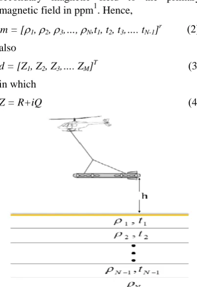
parameters vector, and f is the forward function under investigation. In one-dimensional modelling for a N-layered earth model, as can be seen in Figure 1, i and ti,
3 respectively, denote the resistivity (ohm. meter) and thickness of the earth layers (metres), comprising a model parameter vector. Thus, the number of the model’s parameters is P=2N-1. The data vector is also composed of the real part (R) and the imaginary part (Q) of the ratio of the secondary magnetic field to the primary magnetic field in ppm1. Hence,
( 2 ) m = [1, 2, 3,…, N,t1, t2, t3,…. tN-1]
r
also
( 3 ) d = [Z1, Z2, Z3,…. ZM]
T
in which
( 4 ) Z = R+iQ
Fig. 1. A basic diagram of a one-dimensional N-layer half-space earth model.
Among the various configurations of transmitter and receiver coils, three of them - namely horizontal coplanar (HCP), vertical coplanar (VCP) and vertical coaxial (VCA) systems - are frequently used in practical HEM surveys [13]. In this paper, however, the HCP coil system is considered as providing the most reliable modelling work on a multi-layered earth model (e.g., Huang and Fraser (2003) and Siemon et al. (2009a)) and as such this configuration is used. The EM response of a layered half-space earth model for dipole source excitation in the form of a HCP system at a height h above the layered half-space is given by the forward operator in the following relation [14].
1. Parts per million
0
s p
s 2 A h 3
0 0
0
0 Z
Z ( r )[ ppm ] R iQ
Z
r R ( , , ,t ) e J ( r )d
A
(5) in which Zs and Zp are secondary and primary
magnetic fields, respectively, at the receiver coil location, h is the bird’s height from the ground, R and Q are in-phase (real) and out-of-phase (imaginary) components of data,
i 1 is the imaginary number, r is the distance between the transmitter and the receiver coils, is the integral’s variable,J0 is
a zero-order Bessel function of the first kind, and is the angular frequency. A0 can be
calculating by the following formula.
( 6 )
2 2 1 / 2
0
0 0 0 r1
0 i
A ( )
in which 0 , 0, and 0, are, respectively, the
resistivity, magnetic permeability and electric permittivity of the free space, and r1=1/0is
the relative magnetic permeability of the first layer that has its own magnetic permeability (1) .If the area under investigation has no
noticeable magnetic anomaly, it can be assumed that 0 n or, in other words, that
the relative magnetic permeability of all the layers of the model is equal to one [5]. To find the parameters of the layered earth, we need the reflection coefficient R0, which can be
obtained through the following relation [14]. ( 7 )
0 1 1 0 1 r1 0
0
0 1 1 0 1 r1 0
B A B A
R
B A B A
The parameter B1 and - following that - the
reflection coefficient R0 are then given by the
following recursive relation.
( 8 )
2 1 1 1
1 1
1 2 1 1
B A tanh( A t )
B A
A B tanh( A t )
In addition, for the nth layer
( 9 )
n 1 n n n
n n
n n 1 n n
B A tanh( A t )
B A
A B tanh( A t )
( 10 ) 2 2 1 / 2
0
n 0 0
n i
A ( )
4 ( 11 ) 2 2 1 / 2 0
N N 0 0
N i
A B ( )
Using Relations 8-11, one can accurately determine the reflection coefficient R0 of
Relation 7. However, the forward equation in Relation 5 is a form of Hankel integral, which follows from the general form below [15].
( 12 ) n
0
f ( r )
k ( )J ( r )d In this integral, k() is the transformed kernel function and Jn(r) is the n
th
-order Bessel function of the first kind. Various numerical methods have been proposed for solving this integral form. In this study, the FHTs method with 120-fold weighted coefficients introduced by Guptasarma and Singh (1997) is used to solve Equation 5. Using these coefficients, the above-mentioned integral can be written as a sum of multiple products. ( 13 ) n i i i 1 1
f ( r ) k ( )W
r
Using this method, the forward equation in Relation 5 would become,
( 14 ) 120 2 i i 1
Z R iQ r k ( )W
By comparing Relation 13 with Relation 5, the kernel function k() is given as follows.
( 15 )
0
3 2 A h
0 0
k ( )
R
e
A
Next, using Relation 14, we will be able to find the forward modelling response of the model.
3. Sensitivity matrix calculations
In most geophysical problems, the relation between the data and the model’s parameters is a nonlinear one. In a problem with M data and P parameters, the relation between each datum di with the model’s parameters mi is
described using a nonlinear function fi .
( 16 ) di = fi (m1,m2,m3,…,mp) = fi(m)
Relation 5 shows that the forward equation under investigation is fully nonlinear. The
main idea in solving this kind of problem would be to use a Taylor series expansion of the forward function fi (m) around an initial
guess to linear the equation in the neighbourhood of this initial model. In the next step, by improving on this model and repeating a similar operation, we will obtain a model whose response fits with the observed data in a least squares sense. Thus, by neglecting derivatives of the second-order and higher, we will have the Taylor expansion of the following equation [16].
( 17 )
d = J.m
where d is a vector of difference between the measured (real) data and the response of the initial model, m is the model’s improvement in each iteration (i.e., the difference between the updated and initial model parameters) and is the Jacobian partial derivative or sensitivity matrix, which can be obtained through the following relation.
( 18 ) i ij j f ( m )
J , i 1, 2 ,3 ,...M , j 1, 2 ,3 ,...P m
Or, in other words
(
19
)
1 1 1
1 2 p
2 2 2
1 2 p
M P
M M M
1 2 p
f f f
...
m m m
f f f
...
m m m
J
f f f
...
m m m
5 higher accuracy. As an N-layer earth model (Fig. 1) is considered, all of fi s are the same
and are derived from Relation 5. By looking at this relation, it should be clear that the only term dependent on the model’s parameters is the reflection coefficient R0 Hence.
( 20 ) 0
3 2 A h
3 0
i
0 0
0
i i 0
R f
r ( ) e J ( r )d
m m A
Furthermore, with consideration to Relation 4, we have
( 21 )
0 0 1
j 1 j
R R B
.
m B m
( 22 ) 0 0 2
1 1 0
R 2 A
B ( B A )
in which mj could be either j or tj . Using
Relations 8-11 and the chain differentiation rule, we have
( 23 ) j 1 j j 3
1 1 2
j 2 3 4 j j j
B B A
B
B B B
. . ... . .
B B B B A
( 24 ) j 1 j 3
1 1 2
j 2 3 4 j j
B B
B
B B B
. . ... .
t B B B B t
For the calculation of the derivatives of type n
n 1 B B
that appear in the above relations,
and with respect to Relations 9 and 10, one can show that
( 25 ) 2
n n
2 2 2
n 1 n n n n n
B A
B cosh ( A t )[ A tanh ( A t )]
and also ( 26 ) 2 2
j j 1 j j j j j j j
j
2 j j 1 j j
2
B [ B 2 A tanh( A t ) A t sec h ( A t )]
A V
[1 t B sec h ( A t )]U
V where ( 27 ) V = Aj + Bj+1 Aj tanh(Ajtj)
( 28 ) 2
j j 1 j j j j
U A B A t tan( A t )
It must be noted that in the last layer BN=AN, and hence when j=N, we have
( 29 ) j j B 1 A
For calculating the last terms of Relations 23 and 24, using Relations 9 and 10, we have
( 30 )
j 0
j j j
A i 2 A ( 31 )
3 2 2
j j j j j 1 j j
1
2 j
[ A sec h ( A t )]V [ A B sec h ( A t )]U B t V
Finally, using the recursive Relations 21-31, 0
j R m
could be obtained and substituted in
Eq. 20. The integral in Relation 20 is also in the form of Hankel integrals of Relation 12. Hence, in calculating it, the FHTs with 120-fold weighted coefficients introduced by Guptasarma and Singh (1997) are used. With respect to Relation 13, we will have the following: ( 32 ) 120 2 i i j i 1
f
r k ( )W
m
where its Kernel function is
( 33 ) 0
3 2 A h 0
j 0 0 R
k ( ) e
m A
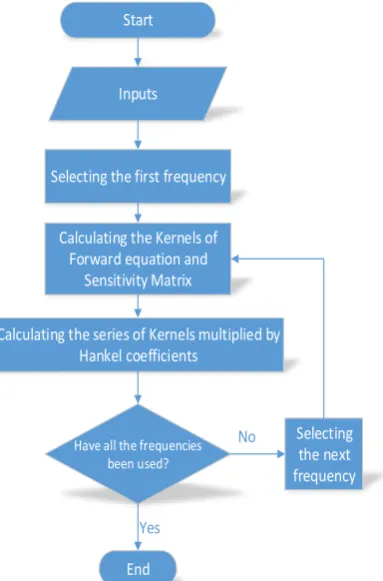
4. An algorithm for the simultaneous calculation of the forward modelling and sensitivity matrix
6 In this algorithm, as Figure 2 illustrates, first all of the required input parameters, including the number of layers, the resistivity and thickness of each layer, the frequencies being used, the flight altitude, the coils distance and the Hankel coefficients are recalled. Next, using Relations 15 and 33, the kernel functions must be calculated for the selected frequency. Finally, using the multiplication sigma of Relations 14 and 32, the values of the forward (synthetic) data and the elements of the sensitivity matrix will be computed and saved. The process will be applied to all the functional frequencies.
Start
Inputs
Selecting the first frequency
Calculating the Kernels of Forward equation and
Sensitivity Matrix
Calculating the series of Kernels multiplied by Hankel coefficients
Have all the frequencies been used?
Selecting the next frequency
No
End
Yes
Fig. 2. A simple flowchart of the proposed algorithm for the simultaneous calculation of the forward
modelling and sensitivity matrix.
5. Results and discussion
In this section, the results of the proposed algorithm are compared with those obtained by the BGR Centre’s software using two synthetic models. First, the results of the forward modelling for the model in Figure 3 will be investigated.
Fig. 3. A sketch of the layering of a four-layered synthetic model.
The synthetic data of this model has been considered by Siemon and his colleagues [6]. The aforementioned model is a four-layered model with a respective specific resistivity of 200, 100, 5 and 1,000 ohm-meter. The first, second and third layers have each a thickness of 20, 30 and 10 metres, respectively. The functional frequencies are 387, 1,820, 8,225, 41,550 and 133,200 Hz. The distance between the coils and the helicopter’s flight altitude, respectively, are 8 and 30 metres. In Table 1, we have outlined the results of 1D forward modelling for the proposed algorithm and those provided by the BGR Centre software [6] at a site located on the left part of the model.
Table 1. The results of 1D forward modelling for the proposed algorithm and those produced by the BGR
software.
Forward modeling
Data of the proposed algorithm
Data of the BGR Software Frequency(Hz) R(ppm) Q(ppm) R(ppm) Q(ppm)
387 21.8 68.36 21.8 68.36 1820 129.1 164.35 129.1 164.4 8225 280.42 291.45 280.4 291.5 41550 734.95 747.46 734.7 747.4 133200 1506.18 1046.81 1506 1047
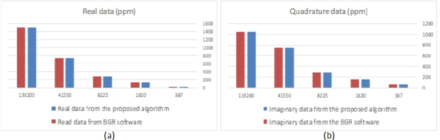
Figure 4 another way of comparing the real and imaginary components of the synthetic data which have been computed by the 1D forward modelling of the proposed algorithm and from the BGR Centre software.
With respect to Table 1 and Figure 4, one can conclude that the results of the proposed algorithm are in close agreement with those of the BGR Centre software.
7 layers, respectively, is 100 and 20 ohm-meter. The thickness of the first layer is 40 metres. The flight altitude and the distance between the coils have been set to 30 and 8 metres,
respectively. It has also been supposed that the data have been surveyed in five frequencies: 900, 1,800, 7,200, 57,600, 133,200 Hz.
Fig. 4. Comparison of the 1D forward data from the proposed algorithm and the BGR software: a) real data, and b) imaginary data.
Fig. 5. A sketch of the layering of the two-layered model.
The proposed algorithm produced the sensitivity matrix as Relation 34. In addition, the BGR Centre software gives the sensitivity matrix as Relation 35.
34 )
0.168630052 2.307556506 1.233126203
0.382572998 2.817244513 2.310850482
1.774434761 1.695683674 4.461238981
8.093572747 0.322332069 1.667932774
8.364728 0.045660611 0.093729348
0.622167035 0.83915142
J
1.505919931
1.076951435 0.126277744 1.711578762
2.75713792 1.796732719 0.562416015
1.942099699 0.155828341 0.53428438
0.24964686 0.028788255 0.387795832
( 35 )
0.168630043 2.307556368 1.233126056
0.38257298 2.817244316 2.310850236
1.774434695 1.695683537 4.461238644
8.09357294 0.322332169 1.667933246
8.364727538 0.04566057 0.093729256
0.622167018 0.83915147
J
5 1.505919817
1.076951407 0.126277799 1.711578662
2.757137865 1.796732616 0.56241588
1.942099815 0.155828423 0.534284438
0.249646814 0.02878823 0.387795493
8 Since there are 10 data in five frequencies (comprising five real and five imaginary components) and the number of parameters is three, the resulting matrix is a 10×3 matrix whose first and second columns are, respectively, the derivatives of each resistivity of 100 and 20 ohm-meter, and its third column is the derivative of the 40 metre thickness of the first layer. Furthermore, the first five rows of the matrix are the derivatives of the real parts, and the second five rows those of the imaginary parts. A comparison of the two resulting matrices shows that the results from the proposed algorithm are in high conformity with those of the BGR Centre software.
6. Conclusion
In this study, first, the relations of the 1D forward modelling of helicopter-borne frequency domain electromagnetic data were investigated. As there is no analytic solution for the integrals in these relations, the fast transforms using Guptasarma and Singh’s (1997) digital linear filter coefficients have been used to solve them numerically. Next, by the analytic calculation of the partial derivatives of the forward equation with respect to the model’s parameters and the FHTs method, the required relations for constructing the sensitivity matrix were obtained. Following this, an efficient algorithm for the simultaneous calculation of the two parts was elaborately designed to speed up the required computation. Finally, the obtained results of this study were compared with those of the BGR Centre software for two synthetic models. This comparison has shown that the results of the proposed algorithm for the 1D forward modelling and sensitivity matrix calculations are in strong agreement with those of the BGR software.
Acknowledgements
The authors are grateful to Dr Bernhard Siemon for providing the results of the BGR Centre software computations for the required models.
References
[1] Ward, S.H., and Hohmann, G.W. (1997).
Electromagnetic theory for geophysical
applications, Nabighian MN (ed) Electromagnetic methods in applied geophysics, 1, Theory: Soc. Exp. Geophys., pp. 130–311.
[2] Sengpiel, K. P. and Siemon, B. (2000). Advanced inversion methods for airborne
electromagnetic exploration. Geophysics,
65(6), pp. 1983–1992.
[3] Zhang, Z., Routh, P.S., Oldenburg, D.W., Alumbaugh, D.L. and Newman, G.A. (2000). Reconstruction of 1-D conductivity from dual-loop EM data, Geophysics, 65, pp. 492–501.
[4] Farquharson, C.G., Oldenburg, D.W. and Routh, P.S. (2003). Simultaneous 1D inversion
of loop-loop EM data for magnetic
susceptibility and electrical conductivity,
Geophysics, 68(6), pp. 1857–1869.
[5] Huang, H. and Fraser, D.C. (2003). Inversion of helicopter electromagnetic data to a magnetic conductive layered earth, Geophysics, 68(4), pp. 1211–1223.
[6] Siemon, B., Auken, E. and Christiansen, A.V. (2009a). Laterally constrained inversion of
helicopter-borne frequency-domain
electromagnetic data. Journal of Applied
Geophysics, 67(3), pp. 259–268.
[7] Arab-Amiri, A.R., Moradzadeh, A.,
Fathianpour, N. and Siemon, B. (2010a). Inverse modeling of HEM data using a new
inversion algorithm. Journal of Mining
Environment, 1, pp. 9–20.
[8] Shirzaditabar, F. and Oskooi, B. (2010). Recovering 1D conductivity from AEM data using Occam inversion, Journal of Earth Space Physics, 37(3), pp. 47–58.
[9] Shirzaditabar, F., Bastani, M. and Oskooi, B. (2011a). Imaging a 3D geological structure from HEM, airborne magnetic and ground ERT data in Kalat-e-Reshm area, Iran, Journal of Applied Geophysics, 75, pp. 513–522.
[10] Abedi, M., Norouzi, G.H., Fathianpour, N. and Gholami, A. (2013). Geological structure imaging from airborne electromagnetic and magnetic data, a case study in Kalat-e-Reshm area, Iran. Arabian Journal of Geosciences, pp. 1–11, DOI 10.1007/s12517-013-1143-7.
[11] Sengpiel, K.P. and Siemon, B., (1998). Examples of 1-D inversion of multifrequency HEM data from 3-D resistivity distributions, Exploration Geophysics, 29(2), pp. 133–141.
[12] Johansen, H.K. and Sorensen, K. (1979). Fast Hankel transforms, Geophysical Prospecting, 27, pp. 876– 901.
9
thesis, Department of Earth Sciences, University of Aarhus.
[14] Siemon, B., Christiansen, A.V. and Auken, E.
(2009b). A review of helicopter-borne
electromagnetic methods for groundwater exploration, Near Surface Geophysics, 7(5-6), pp. 629–646.
[15] Guptasarma, D. and Singh, B. (1997). New digital linear filters for Hankel J0 and J1 transforms, Geophysical prospecting, 45(5), pp. 745–762.