On the Estimation of Empty cell Probabilities in a Contingency Table

(1)

O

N

T

H

E

S

T

I

M

A

T

I

O

N

O

F

E

M

P

T

Y

C

E

L

P

R

O

B

A

B

I

L

I

T

I

E

S

I

N

A

C

O

N

T

I

N

G

E

N

C

Y

T

A

B

L

E

O

y

e

y

e

m

i

G

.

M

.

11

a

n

d

M

b

a

e

y

i

G

.

C

.

22

1

Department of Statistics, University of Ilorin, P. M. B. 1515, Ilorin, Kwara State, Nigeria

2

Department of Mathematics/Computer Science/Statistics/Informatics, Federal University Ndufu-Alike Ikwo, P. M. B. 1010, Abakaliki, Ebonyi State,Nigeria

Corresponding Author: Oyeyemi G. M., [email protected]

ABSTRACT: In this paper, an Independent Binary Model

(IBM) is proposed. It is aimed at estimating cell probabilities in an r x c contingency table when some of the cells have zero count. Existing methods in this situation are either subjective or based on arbitrary decision of the researcher. The IBM is applied to sets of simulated data for various combinations of categorical variables. It is pointed out that the IBM could be an alternative for such situations especially when the result is needed for further analysis.

KEYWORDS: Cell probabilities, Categorical variables, Independent Binary Model, Zero count.

1. INTRODUCTION

In dealing with contingency tables, one of the problems encountered is that of empty (or zero count) cell frequency. The empty cell could be as a result of sampling variability and the relative smallness of the cell probability. This is commonly referred to as sampling zero ([Fie70]). It may also be that observations for certain cells in a contingency table were missing or truncated ([BF69]; [LS85]) or that certain combinations of the variables are impossible and thus there is zero (no count) probability attached to these cells. This is known as apriori zero. Whereas increasing the sample size will take care of the sampling zero, it may or wouldn’t for the apriori zero.

The problem of zero cell frequency (and the corresponding zero probability) could be seen noticeably in the inability to obtain Odd ratio value, non-convergence in logistic regression, difficulty in the chi-square test for association, inability to perform test for proportion in two samples, and, ultimately, in classification and discriminant analysis.

Discriminant analysis involving c-categorical (including binary) variables requires setting up contingency table of multinomial cells arising from cross tabulation of the categorical variables thus defining unique patterns for all the cells of the contingency table. The probability of each pattern is determined by taking the proportion of observations

with such pattern. This is only possible when the frequencies of all the pattern (or observations in each cell) are non-zero. When this is not the case, desired analysis becomes difficult. Rather than resorting to intuitions, or arbitrary/non-consistent choice of methodology, it is worth to look for a way around this problem. This is what this work seeks to examine.

Dureh et al ([DCT16]) in solving the problem of non-convergence in logistic regression on contingency table tables with zero cell counts, suggested modifying the data by replacing the zero count by value 1 and doubling a corresponding non-zero count.

Agrestic ([Agr02]) in calculating the sample odd ratio or if any count is 0, the Agresti’s estimator of the Odd Ratio (OR)

where a, b, c, and d are cell counts. That is, 0.5 is added to every cell of the contingency table.

With the problem of zero cell in the chi-square test for association for a r x c contingency table, Watson ([Wat56]) noted that the observed cell frequencies are sample N from a multinomial population and then gave intuitively that a missing (or zero cell count) value x in a contingency table with R-rows and C-columns can be computed using

if and only if the zero count occurs in row and column or row column otherwise

where is the cell of the row and is the cell of the column in which the zero count occur.

(2)

obtaining this increased sample size is very difficult especially in the zero cell case.

Dobra et al ([DTW06]) in a Bayesian framework computed posterior distribution for unobserved (zero) cell counts and parameters underlying models for cell probabilities in tables with sets of fixed margins.

A popular literature ([Krz75]; [Krz80]; [Krz86]; [AK90]) for discriminant analysis with mixed variables uses the Iterative proportional fitting procedure ([Hab72]; [RS95]; [Fab14]).

The Iterative Proportional Fitting (IPF), sometimes referred to as “Raking” is used to adjust a table of data cells such that they add up to selected totals for both the columns and rows of a table. By this adjustment, cell probabilities are determined wherein cell counts are repeatedly and proportionally adjusted to equal margin totals until selected (or desired) level of convergence is reached. The IPF procedure employs a log-linear model while rescaling the cells of a contingency table. However, Norman ([Nor99]) noted that IPF cannot work if any of the marginal cell values are equal to zero. That is, if for the given margin, a cell has zero count then the IPF becomes impracticably inapplicable. If this occurs, Touloumis ([Tou14]) suggests making the value for such cells very small compared to all of the other cells in the marginal. This agrees with David ([Dav92]), Fabian ([Fab14]) and Xu et al ([XSS16]) who noted that the IPF needs adequate sample size in order to be reliable. In using the IPF, Eddie ([Edd08]) noted that, no adjustment will be made to cell with a value of zero. With these, the IPF as has been used in discriminant analysis of mixed variables may not have been a dependable in situation of zero cell count.

2. THE PROPOSED ESTIMATION PROCEDURE

Let be a p-dimensional random vector of Bernoulli variables. A particular value X, denoted by is called a response pattern. Each is defined by a unique pattern. This pattern consists of 0’s and 1’s. The 0’s and 1’s are used to indicate presence/absence of entity of interest or possession/non-possession of a particular attribute. Denote with the probability that has the response pattern . By writing in terms of the probability mass function (pmf) of Bernoulli distribution and combining the independent law of probability, the Independent Binary Model (IBM) is proposed as follows;

Where is the set of all patterns with . From the above, is the estimated probability of each response pattern which corresponds to the probability of any given observation falling into cell c of the contingency table. With the IBM, probability of each response pattern necessarily no longer depend on the proportion (obtained using the number of observations with such response pattern) of response pattern but the result obtained with the estimation procedure using the IBM. The IBM is related to the First Order Bahadur Model ([Bah61]). It was used by Moore ([Moo73]) and Asparoukhov & Stam ([AS96]) for classification using only binary variables, Fitzmaurice et al ([F+06]) estimating regression parameters for longitudinal binary data and was reviewed by Heumann ([Heu14]). Carefully written program will execute the estimation procedure with minimum computer time as such speed and accuracy is not lost.

2.1 Justification for using the IBM

Though it has been used by some authors in classification, none has used it for probability estimation purpose and hence the objective of this work; estimation of zero cells probabilities. It has only been used for binary variable case but this work will extend it to incorporate variables that have more than two states. It follows a known probability function and it is based on valid probability law.

3. SIMULATION AND APPLICATION

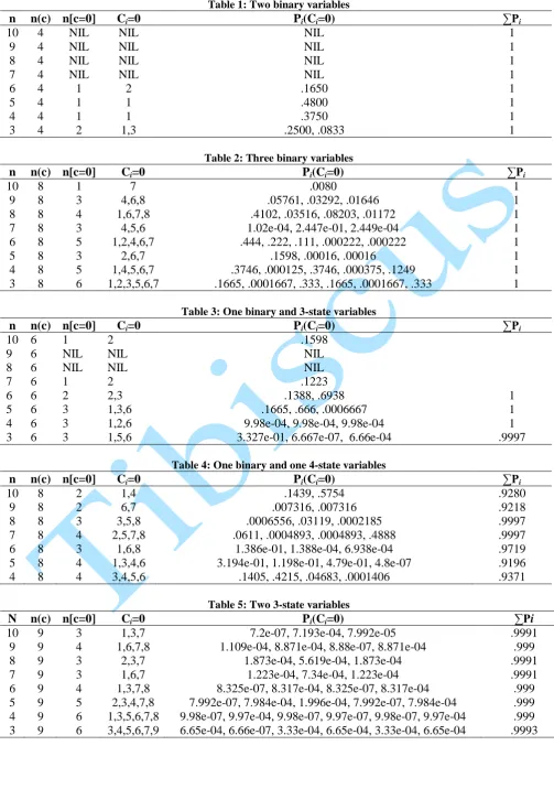
Categorical variables were simulated for various small sizes and cross classified into a contingency table. The essence of considering only small samples is to give room for occurrence of cells with zero count. The IBM was then used to estimate probabilities for the zero count cells and in that process adjust other cell probabilities by re-estimating them using the IBM. Results are presented in each table according to number of categorical variables cross-classified.

4. RESULTS AND DISCUSSION

4.1 Results

(3)

Table 1: Two binary variables

n n(c) n[c=0] Ci=0 Pi(Ci=0) ∑Pi 10 9 8 7 6 5 4 3 4 4 4 4 4 4 4 4 NIL NIL NIL NIL 1 1 1 2 NIL NIL NIL NIL 2 1 1 1,3 NIL NIL NIL NIL .1650 .4800 .3750 .2500, .0833 1 1 1 1 1 1 1 1

Table 2: Three binary variables

n n(c) n[c=0] Ci=0 Pi(Ci=0) ∑Pi 10 9 8 7 6 5 4 3 8 8 8 8 8 8 8 8 1 3 4 3 5 3 5 6 7 4,6,8 1,6,7,8 4,5,6 1,2,4,6,7 2,6,7 1,4,5,6,7 1,2,3,5,6,7 .0080

.05761, .03292, .01646 .4102, .03516, .08203, .01172 1.02e-04, 2.447e-01, 2.449e-04 .444, .222, .111, .000222, .000222

.1598, .00016, .00016

.3746, .000125, .3746, .000375, .1249 .1665, .0001667, .333, .1665, .0001667, .333

1 1 1 1 1 1 1 1

Table 3: One binary and 3-state variables

n n(c) n[c=0] Ci=0 Pi(Ci=0) ∑Pi 10 9 8 7 6 5 4 3 6 6 6 6 6 6 6 6 1 NIL NIL 1 2 3 3 3 2 NIL NIL 2 2,3 1,3,6 1,2,6 1,5,6 .1598 NIL NIL .1223 .1388, .6938 .1665, .666, .0006667 9.98e-04, 9.98e-04, 9.98e-04 3.327e-01, 6.667e-07, 6.66e-04

1 1 1 .9997

Table 4: One binary and one 4-state variables

n n(c) n[c=0] Ci=0 Pi(Ci=0) ∑Pi 10 9 8 7 6 5 4 8 8 8 8 8 8 8 2 2 3 4 3 4 4 1,4 6,7 3,5,8 2,5,7,8 1,6,8 1,3,4,6 3,4,5,6 .1439, .5754 .007316, .007316 .0006556, .03119, .0002185 .0611, .0004893, .0004893, .4888

1.386e-01, 1.388e-04, 6.938e-04 3.194e-01, 1.198e-01, 4.79e-01, 4.8e-07

.1405, .4215, .04683, .0001406

.9280 .9218 .9997 .9997 .9719 .9196 .9371

Table 5: Two 3-state variables

N n(c) n[c=0] Ci=0 Pi(Ci=0) ∑Pi 10 9 8 7 6 5 4 3 9 9 9 9 9 9 9 9 3 4 3 3 4 5 6 6 1,3,7 1,6,7,8 2,3,7 1,6,7 1,3,7,8 2,3,4,7,8 1,3,5,6,7,8 3,4,5,6,7,9

7.2e-07, 7.193e-04, 7.992e-05 1.109e-04, 8.871e-04, 8.88e-07, 8.871e-04

1.873e-04, 5.619e-04, 1.873e-04 1.223e-04, 7.34e-04, 1.223e-04 8.325e-07, 8.317e-04, 8.325e-07, 8.317e-04 7.992e-07, 7.984e-04, 1.996e-04, 7.992e-07, 7.984e-04 9.98e-07, 9.97e-04, 9.98e-07, 9.97e-07, 9.98e-07, 9.97e-04 6.65e-04, 6.66e-07, 3.33e-04, 6.65e-04, 3.33e-04, 6.65e-04

(4)

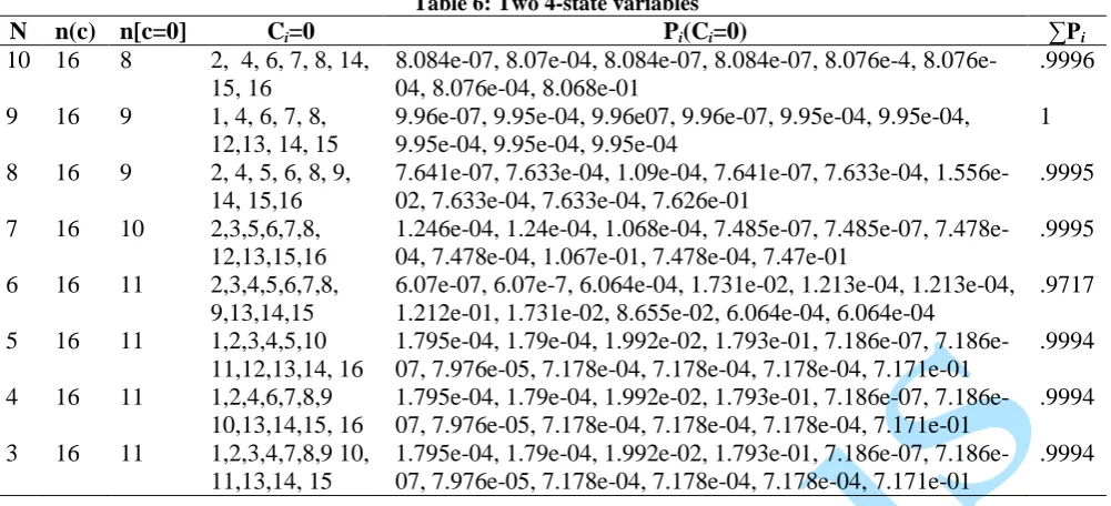
Table 6: Two 4-state variables

N n(c) n[c=0] Ci=0 Pi(Ci=0) ∑Pi 10

9

8

7

6

5

4

3 16

16

16 8

9

10

11

2, 4, 6, 7, 8, 14, 15, 16

1, 4, 6, 7, 8, 12,13, 14, 15 2, 4, 5, 6, 8, 9, 14, 15,16 2,3,5,6,7,8, 12,13,15,16 2,3,4,5,6,7,8, 9,13,14,15 1,2,3,4,5,10 11,12,13,14, 16 1,2,4,6,7,8,9 10,13,14,15, 16 1,2,3,4,7,8,9 10, 11,13,14, 15

8.084e-07, 8.07e-04, 8.084e-07, 8.084e-07, 4, 8.076e-04, 8.076e-8.076e-04, 8.068e-01

9.96e-07, 9.95e-04, 9.96e07, 9.96e-07, 9.95e-04, 9.95e-04, 9.95e-04, 9.95e-04, 9.95e-04

7.641e-07, 7.633e-04, 1.09e-04, 7.641e-07, 7.633e-04, 1.556e-02, 7.633e-04, 7.633e-04, 7.626e-01

1.246e-04, 1.24e-04, 1.068e-04, 7.485e-07, 7.485e-07, 7.478e-04, 7.478e-7.478e-04, 1.067e-01, 7.478e-7.478e-04, 7.47e-01

6.07e-07, 6.07e-7, 6.064e-04, 1.731e-02, 1.213e-04, 1.213e-04, 1.212e-01, 1.731e-02, 8.655e-02, 6.064e-04, 6.064e-04

1.795e-04, 1.79e-04, 1.992e-02, 1.793e-01, 07, 7.186e-07, 7.976e-05, 7.178e-04, 7.178e-04, 7.178e-04, 7.171e-01 1.795e-04, 1.79e-04, 1.992e-02, 1.793e-01, 07, 7.186e-07, 7.976e-05, 7.178e-04, 7.178e-04, 7.178e-04, 7.171e-01 1.795e-04, 1.79e-04, 1.992e-02, 1.793e-01, 07, 7.186e-07, 7.976e-05, 7.178e-04, 7.178e-04, 7.178e-04, 7.171e-01

.9996

1

.9995

.9717

.9994

4.2 Discussion

Tables 1 – 6 above present results of estimation using the IBM on various combinations of categorical variables. Note that the variables includes those with more than two states, as such, the IBM can be extended to incorporate not just binary but categorical variables with more than two states. Probability values decreases as we estimate cell down the rows. That is, higher probability values occurs at the first cell, the second row (by row) has the next highest, the third the next and so on. Some values seem to exhibit a pattern especially when the occurrence of the zero has a pattern. Due to truncation error, the probabilities may not always sum to exactly 1 but it will do when rounding up from 3-significant values. The IBM would be more effective in situation where numbers of empty cell resulting from the number of categorical (including binary) variables available are many. The more the empty cell, the less tendency of the estimated probabilities to sum to 1.Probabilities summed to exactly 1 for the 3-binary case but such was not the case for 1-binary and one 4-state categorical even though both have 8 cells. This implies that, with transforming 3 or more state categorical variable into binary, probabilities slowly sum to 1.For the 4-state variable, convergence (in terms of unchanging values of cell probabilities) was attained when observation was 5 or less.

5. CONCLUSION

It has been shown that for contingency tables having some zero count cells, the direct maximum likelihood estimation procedure becomes difficult. Unlike the iterative proportional fitting procedure

on the grand total and can be used for variables with more than two states. It is however similar with the IPF procedure in that it makes re-adjustment of the cell probabilities. As it is intended to use the IBM to estimate probabilities corresponding to cells with zero count, results obtained using the IBM attest to its importance.

REFERENCE

[Agr05] Agresti A. - Categorical Data Analysis. John Wiley & Sons, New York, USA. 70 -71, 2002.

[AK00] Asparoukhov O., Krzanowski W. J. -

Non-parametric smoothing of the

location model in mixed variable

discrimination. Statistics and

Computing, 10, 289 – 297, 2000.

[AS96] Asparoukhov O. K., Stam A.

-Mathematical Programming

formulations for Two-group

Classification with Binary Variables.

IIASA working paper, IIASA, Axenburg, Austria. WP-96-092, 1996. [Bah61] Bahadur R. R. - On classification

based on responses to n dichotomous items. H. Solomon (Ed.), Studies in Item Analysis, Stanford University Press, New York, 1961.

[BF69] Bishop Y. M. M., Fienberg S. E. -

Incomplete Two-Dimensional

(5)

[Dav92] David W. S. W. - The Reliability of using the Iterative Proportional Fitting

Procedure.The Professional

geographer, 3(44), 340 – 348.

Doi.org/10.1111/j:0033-0214.1992.00340.x, 1992.

[DCT16] Dureh N., Choonpradub C., Tongkumchum P. - An Alternative method for Logistics Regression on Contingency Tables with Zero Cell

Counts. Songklanakarin J. Sci.

Technol., 38(2), 171 – 176, 2016.

[DTW06] Dobra A., Tebaldi C., West M. - Data augmentation in multi-way contingency tables with fixed marginal totals.

Journal of Statistical Planning and Inference, 136, 355 – 372, 2006.

[Edd08] Eddie H. - Iterative Proportional Fitting for a Two-Dimensional Table.

Alaska Department of Labor and Workforce Development. Alaska, 2008.

[Fab14] Fabian P. R. - Termination of the

Iterative Proportional Fitting

Procedure.Statistics & Probability Letters. 92, 59 – 64, 2014.

[Fie70] Fienberg S. E. - Quasi-Independence and Maximum Likelihood Estimation in

Incomplete Contingency Tables.

Journal of the American Statistical Association, 332(65), 1610 – 1616.

[F+06] Fitzmaurice G. M., Lissitz S. R., Ibrahim J. G., Geller R., Lipshultz S. - Estimation in regression models for longitudinal binary data with outcome-dependent follow-up. Biostatistics, 3(7), 469 – 485, 2006.

[Hab72] Haberman S. J. - Log-Linear fit for Contingency Tables. Algorithm AS51.

Applied Statistics, 21, 218 – 225, 1972.

[Heu14] Heumann C. - The Bahadur Model.

Wiley StatsRef: Statistics Reference

Online. DOI:

10.1002/9781118445712.stat07877, 2014.

[Krz75] Krzanowski W. J. - Discrimination and Classification Using both Binary and Continuous Variables. Journal of

the American Statistical Association, 70, 782-790, 1975.

[Krz80] Krzanowski W. J. - Mixtures of Continuous and Categorical Variables in Discriminant Analysis. Biometrics, 36, 493-499, 1980.

[Krz86] Krzanowski W. J. - Multiple Discriminant Analysis in the presence of Mixed Continuous and Categorical Data. Comp.&Maths. With Appls., 2(12), 179 – 185, 1986.

[LS85] Little R. J. A., Schluchter M. D. -

Maximum Likelihood Estimation for Mixed Continuous and categorical Data with Missing Values. Biometrika,

3(72), 497 – 512, 1985.

[Moo73] Moore D. H. - Evaluation of Five Discrimination Procedure for Binary variables. Journal of the American Statistical Society, 68(342), 399 –404, 1973.

[Nor99] Norman P. - Putting Iterative

Proportional Fitting on the

Researcher’s Desk. Working paper 99/3. School of Geography, University of Leeds, Leeds, 1999.

[RS95] Radim J., Stanislav P. - On the effective implementation of the Iterative

Proportional fitting Procedure.

Computational Statistics & Data Analysis, 2(19), 177 – 189, 1995.

[Tou14] Touloumis A. - Nonparametric Stein-type shrinkage covariance matrix estimators in high-dimensional setting.

Computational Statistics and Data Analysis, 83, 251 – 261, 2014.

[Wat56] Watson G. S. - Missing and

“Mixed-Up” Frequencies in Contingency Tables. Biometrics, 12(1), 47 – 50, 1956.

[XSS16] Xu P. F., Sun J., Shan N. - Local

Computation of the Iterative