Comparative Study of Stability Range of Proposed PI Controllers for Tidal Current Turbine Driving DFIG

(1)

Published online March 10, 2013 (http://www.sciencepublishinggroup.com/j/ijrse) doi: 10.11648/j.ijrse.20130202.15

Comparative study of stability range of proposed PI

con-trollers for tidal current turbine driving DFIG

Hamed H. H. Aly, M. E. El-Hawary

Department of Electrical and Computer Engineering, Dalhousie University, Halifax, NS, B3H 4R2, Canada

Email address:

[email protected] (H. H. H. Aly), [email protected] (M. E. El-Hawary)

To cite this article:

Hamed H. H. Aly, M. E. El-Hawary. Comparative Study of Stability Range of Proposed PI Controllers for Tidal Current Turbine Driving DFIG. International Journal of Renewable and Sustainable Energy. Vol. 2, No. 2, 2013, pp. 51-62.

doi: 10.11648/j.ijrse.20130202.15

Abstract:

Renewable energy in the power grid system is one of the most important topics in electricity generating now and into the future. The increasing penetration of this type of energy makes it very important for researchers to put the spot on. Tidal current energy is one of the most rapidly growing technologies for generating electric energy. Within that frame, tidal current energy is surging to the fore. The doubly fed induction generator (DFIG) is one of the most commonly used generators associated with tidal current and offshore wind turbines. The aim of the present work is to dedicate control strat-egies for the DFIG, enabling the turbines to act as an active component in the power system. This paper describes the over-all dynamic models of tidal current turbine driving DFIG connected to a single machine infinite bus system and proposed two PI controllers used for improving the power system stability. DFIG is tested for small signal stability analysis. The overall system is verified. The system is tested using different values of controllers coefficients to determine the preferred ranges of values of the controllers coefficients for the system stability. The overall results are discussed and proved the importance of the proposed controllers.

Keywords:

Tidal Current Power, Direct Drive Permanent Magnet Synchronous Generator (DDPMSG), Doubly Fed In-duction Generator (DFIG), Power System Stability

1. Introduction

In recent years, conventional non-renewable electrical energy production has become an increasing concern due to its high costs, limited resources, and negative influence on global warming from CO2 emissions. In response to these challenges, scientists have begun to focus their re-search on renewable energy sources. Renewable energy is generally a clean source of supplying electrical loads, es-pecially in remote and rural areas. Wind energy is one of the most common and rapidly growing renewable energy sources. Wind energy is produced from air motion caused by the uneven heating of the earth’s surface by the sun. While wind turbines are associated with negative issues such as noise, visual impacts, erosion, birds and bats being killed, and radio interference, it is still an extremely useful form of energy in rural areas where access to utility trans-mission facilities is limited. Moreover, the use of wind energy reduces greenhouse gas emissions and positively impacts climate change due to fossil fuel replacement. Worldwide wind capacity is growing fast and may reach up

to 1 million MW by 2050. This means that wind energy integration will become an important factor in the stability of the electric grid. Thus, there is a need for a ‘smart’ grid that is able to work through any disturbance and supply high quality electric energy to consumers. To date, however, wind power as an energy source is intermittent, challenging to predict, and requires using some form of storage to inte-grate it into the electric grid. New control techniques and improved forecasting methods are helpful in establishing operating practices that will increase the reliability of wind energy supply [1, 2].

(2)

(the speed of the neap tides varies from 2 to 2.5m/s), which happens when the moon and the sun are at right angles and pull seawater in different directions. Nova Scotia’s Bay of Fundy is characterized by high tides that can reach up to 17 meters. The electrical-side layout and modeling approaches used in tidal in-stream systems are similar to those used for wind and offshore wind systems. The speed of water cur-rents is lower than wind speed, while the water density is higher than the air density and as a result wind turbines operate at higher rotational speeds and lower torque than tidal in-stream turbines which operate at lower rotational speed and high torque [1-5].

The easier predictability of the tidal in-stream energy re-source makes it easier to integrate in an electric power grid. Recognizing that future ocean energy resources are avail-able far from load centers and in areas with limited grid capacity will result in challenges and technical limitations. With the growing penetration of tidal current energy into the electric power grid system, it is very important to study the impact of tidal current turbines on the stability of the power system grid and to do that we should model the overall system. The model of the ocean energy system con-sists of three stages. The first stage contains the fluid me-chanical process. The second stage consists of the mechan-ical conversion and depends on the relative motion be-tween bodies. This motion may be mechanical transmission and then using mechanical gears or may be depending on the hydraulic pumps and hydraulic motors. The third stage consists of the electromechanical conversion to the elec-trical grid [4-8].

DFIG and DDPMSG are the most commonly used gene-rators with tidal current turbines. Different controllers are used for stabilization of DFIG and DDPMSG for both the grid side converter and the generator side converter for offshore wind turbines. Some of these controllers use the generator side converter controller to maintain the rotation-al speed of the generator at an optimrotation-al vrotation-alue, and minimize the core losses; and use the grid side converter controller to maintain the voltage of the DC-link, and control the output reactive power to a certain level. Other controllers use the generator side converter controller for controlling the out-put active power and reactive power, while using the grid side converter controller for controlling the DC-link vol-tage and the terminal volvol-tage of the turbine system [3, 9]. The following sections describe the dynamic model of the whole system including the proposed controllers and the state space representation of the whole system.

Nomenclature

Vtide Tidal current speeds.

Vnt Neap tide speed.

Vst Spring tide speed.

Cs Constant and equals 95 for spring, 45 for neap tide.

Pts Tidal in-stream power.

ρ Density of the water (1025 kg/m3₎

A Cross-sectional area perpendicular to the flow direction.

Tm Mechanical torque applied to the turbine.

A Cross-sectional area perpendicular to the flow direction.

Cp Marine turbine blade design constant in the range of

0.35-0.5.

ωs ,ωr , ωt Stator, rotor electrical angular velocities, and turbine

speed at hub height upstream the rotor.

Te Electrical torque of the generator.

Ds Shaft stiffness damping.

Ht ,Hg Turbine and generator inertia constants.

Ks Shaft stiffness coefficient.

Ɵt ,Ɵr Turbine and generator rotor angles.

β Tidal turbine pitch angle.

S Rotor slip.

d, q Indices for the direct and quadrature axis components.

s, r Indices of the stator and the rotor.

v, R, i, ψ Voltage, resistance, current, and flux linkage of the generator.

, Coefficients for the proportional-integral controller of the pitch controller.

Pg, PDC Active power of the AC terminal at the grid side

con-verter and DC link power respectively.

vDg , vQg D and Q axis voltages of the grid side converter.

iDg ,iQg D and Q axis currents of the grid side converter.

C Capacitance of the capacitor.

vDC , iDC Voltage and current of the capacitor.

Kp1, Kp2,

Kp3

Proportional controller constants for the generator side converter controller

Ki1, Ki2 ,Ki3 Integral controller constants for the generator side

con-verter controller.

iDg, iQg D and Q axis grid currents.

vDg, vQg D and Q axis grid voltages.

Kp4, Kp5,

Kp6

Proportional controller constants for the grid side con-verter.

Ki4, Ki5, Ki6 Integral controller constants for the grid side converter.

Xc Grid side smoothing reactance.

State variable

2. Tidal Current Model using DFIG

This section reviews the dynamic model of the tidal cur-rent turbine system, DFIG, the converter and the proposed controllers.

2.1. The Speed Signal Resource Model

The tidal current speed may be expressed as a function of the spring tide speed, neap tide speed and tides coeffi-cient (Cs). Hence knowing tides coefficoeffi-cient, it is easy to derive a simple and practical model for tidal current speeds as follows [3, 10]:

=

2.2. The Rotor Model

The power (Pts) may be found using: Pts = ½ ρA(Vtide)3.

The turbine harnesses a fraction of this power, hence the power output may be expressed as: Pt = ½ ρCpA(Vtide)3.

(3)

The shaft system may be represented by a two mass sys-tem one for the turbine and the other for the generator as shown:

0.5ρΠ !" #$

ω&

(1)

2Ht

'

= Tt – Ks(ſr-ſt) – Ds (ωr- ωt) ₍₂₎

2Hg

'(

= Te - Ks(ſr-ſt) – Ds (ωr- ωt) ₍₃₎

ſ_tr₌ſ_r_-ſ_t

(4)

ſſ_&)

= ωr- ωt ₍₅₎

There is a ratio for the torsion angles, damping and stiff-ness that need to be considered when one adds a gear box as all above calculations must be referred to the generator

side and calculated as : a= '_'( , *₊ '(

,

- ,

, - ,

a2 ., / =a2/ .. The same model used for the offshore wind is used for tidal in-stream turbines; however, there is a number of differences in the design and operation of marine turbines due to the changes in force loadings, immersion depth, and different stall characteristics. Since the extracted power from the tidal currents is proportional to the area and the cube of the velocity, hence narrow channels is preferred for tidal turbines to extract higher power as the velocity is higher.

2.3. Dynamic Model of DFIG

The DFIG model is developed using a synchronously ro-tating d-q reference frame with the direct-axis oriented along the stator flux position. The reference frame rotates at the same speed as the stator voltage. The stator and rotor active and reactive power are given by [4-10]:

Ps=3/2( vds ids + vqs iqs ) , Pr= 3/2(vdr idr + vqr iqr )

(6)

Pg= Ps + Pr (7)

Qs=3/2(vqs ids - vds iqs ) , Qr=3/2 (vqr idr - vdr iqr )

(8)

The model of the DFIG can be described as:

vds = -Rs ids - ωs ψqs +

0

0&ψ01 (9)

vqs = -Rs iqs + ωs ψds +

0

0&ψ21 (10)

vdr = -Rr idr - s ωs ψqr +

0

0&ψ0) (11)

vqr = -Rr iqr + s ωs ψdr +

0

0&ψ2) (12)

Ψds = -Lss ids - Lm idr , Ψqs = -Lss iqs - Lm iqr (13)

Ψdr = -Lrr idr - Lm ids , Ψqr = - Lrr iqr - Lm iqs (14)

s =( ωs –ωr )/ωs (15)

'(_{= -ω}

s (16)

Where, Lss= Ls+ Lm, Lrr= Lr+ Lm, Ls, Lrand Lmare

the stator leakage, rotor leakage and mutual inductances, respectively. The previous model may be reduced by ne-glecting stator transients and is described as follows:

vds = -Rs ids + Xˈ iqs + ed (17)

vqs = -Rs iqs - Xˈ ids + eq (18)

34

35 6

1

894 : 6 : ;< = > * 4<

6 * ?

?++#<+

(19)

34<

35 6

1

894<6 : 6 : ; = 6 > * 4

* ?

?₊₊# +

(20)

The components of the voltage behind the transient (the internal voltage components of the induction generator) are

4 6' @A

@(( B<+ and 4<

' @A

@(( B +. The stator

reac-tance X = ωs Lss = Xs +Xm, and the stator transient

reac-tance XƟ = ωs (Lss – Lm2/Lrr) = Xs + (Xr Xm)/ (Xr + Xm).

The transient open circuit time constant is To = Lrr/Rr = (Lr +Lm)/Rr, and the electrical torque is Te= (idsiqr-iqsidr)Xm/*.

2.4. The Pitch Controller Model

The pitch controller is used to adjust the tidal current turbine to achieve a high speed magnitude. This may be represented by a PI controller with a transfer function

+C_ED shown in Figure (1).

β=( +C_ED)ωt (21)

0F 0& =

G&

(4)

Figure 1. Pitch angle control block

2.5. The Converter Model

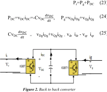
A converter feeds or takes power from the rotor circuit and gives a variable speed (a partial scale power converter used). The rotor side of the DFIG is connected to the grid via a back to back converter. The converter at the side connected to the grid is called the supply side converter (SSC) or grid side converter (GSC) while the converter connected to the rotor is the rotor side converter (RSC). The RSC operates in the stator flux reference frame. The direct axis component of the rotor current acts in the same way as the field current as in the synchronous generator and thus controls the reactive power change. The quadra-ture component of the rotor current is used to control the speed by controlling the torque and the active power change. Thus the RSC governs both the stator-side active and reactive powers independently. The GSC operates in the stator voltage reference frame. The d-axis current of the GSC controls the DC link voltage to a constant level, and the q-axis current is used for reactive power control. The GSC is used to supply or draw power from the grid accord-ing to the speed of the machine. If the speed is higher than synchronous speed it supplies power, otherwise it draws power from the grid but its main objective is to keep the dc-link voltage constant regardless of the magnitude and direction of the rotor power The back to back converter using a DC link is shown in Figure (2). The balanced power equation is given by [13, 14]:

Pr=Pg+PDC (23)

PDC=vDCiDC=-CvDC

HIJ_{, P}

g=vDgiDg+vQgiQg (24)

CvDC

HIJ

= vDgiDg+vQgiQg - vdr idr - vqr iqr (25)

Figure 2. Back to back converter

2.6. Rotor Side Converter Controller Model

The rotor side converter controller used here is repre-sented by four states ( _K, _!, _$and ), _K is related to the difference between the generated power of the stator and the reference power that is required at a certain time, _! is related to the difference between the quadrature axis

gen-erator rotor current and the reference current that is re-quired at a certain time, _$ is related to the difference be-tween the stator terminal voltage and the reference voltage that is required at a certain time, and is related to the difference between the direct axis generator rotor current and the reference current that is required at a certain time [13, 14]. Figure (3) shows the rotor side converter control-ler.

Figure 3. Generator side converter controller

This is described by equations (26-34).

K= Pref -Ps (26)

K= - Ki1/ Kp1x1 +1/ Kp1 iqr_ref (27)

!= iqr_ref -iqr (28)

!= Kp1 K+ Ki1 x1 - iqr (29)

! =- ! / !x2 +1/ ! vqr - ωsLm/ ! ids

-ωsLrr/ !idr + (Lm/ !) idsωr +(Lrr/ !)idrωr

(30)

$= vs_ref - vs (31)

$= - Ki3/ Kp3x3 +1/ Kp3 idr_ref (32)

= idr_ref - idr (33)

=- _! / _!x4 +1/ ! vdr - ωsLm/ ! iqs

-ωsLrr/ !iqr + (Lm/ !) iqsωr +(Lrr/ !)iqrωr

(34)

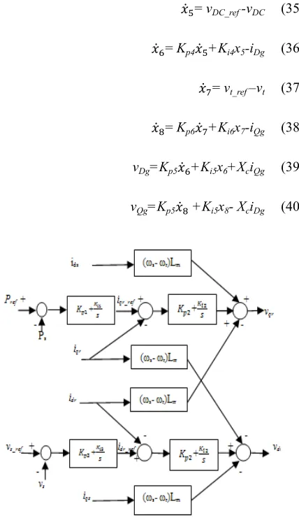
2.7. Grid Side Converter Controller Model

The grid side converter controller used here is repre-sented by four states ( , L, Mand N), x5 is related to the

(5)

differ-ence between the grid terminal voltage and the referdiffer-ence terminal voltage required at a certain time, x6 is a

combi-nation of x5 and direct axis grid current and x8 is a

combina-tion of x6 and quadrature axis grid current as shown in

equations (35-40). Figure (4) shows the grid side converter

controller.

= vDC_ref -vDC (35)

L= Kp4 +Ki4x5-iDg (36)

M= vt_ref –vt (37)

N= Kp6 _M+Ki6x7-iQg (38)

vDg=Kp5 L+Ki5x6+XciQg (39)

vQg=Kp5 _N +Ki5x8- XciDg (40)

Figure 4. Grid side converter controller

3. State Space Representation and

Small Signal Stability Analysis of The

System

In this section we describe the state space representation of the whole system and apply the small signal stability analysis of a single machine infinite bus system for tidal current turbine using DFIG. Small signal stability is the ability of the power systems to remain in synchronism un-der small disturbances. Small signal stability analysis for the power system determines the properties of operation of the system due to small disturbance in the system. This is done by finding the eigenvalues of the system for a small change that may have happened. In this section we perturb each state of the system by a small increment ∆, keeping in mind some assumptions [15]. These assumptions are: ∆2=0,

sin∆=0 and cos∆=1. Using these assumptions we can re-write the state space equations as:

∆ =Q∆ R∆S

∆ for DFIG [∆\ , ∆], ∆#^ , ∆ſ+, ∆4 , ∆4< , ∆ ^ ,

∆ K, ∆ !, ∆ $, ∆ , ∆ , ∆ L, ∆ M, ∆ N _T

The fifteen states of the DFIG are \ , ] , #_^ ,ˈ₊, 4 , 4_<, _^ , _K, _!,

$ , , , L, M and N. Equations (2), (3), and (5) are

used for the drive train. Equations (19) and (20) are used for the generator. Equations (23), (24), and (25) for the DC link give vDC state. Equations from (26) to (34) are used for

the generator side converter controller model and give the states x1 and x2. Equations from (35) to (40) are used for

the grid side converter controller.

4. Effect of Changing the Controllers

Coffecients Values

As the values of the controllers coefficients change, the stability will change. In this section we will try to change the values of the controllers coefficients independently and try to find the relation between the increasing or decreasing of these coefficients independently and the degree of the stability. Also we will try to rank the importance of these coefficients for the stability analysis.

4.1. DFIG Controllers Coefficient

In this section we try to do some computational work that compares the effects of specific parameters change on stability for DFIG. At the end of this section we discuss the preferred ranges of values of the controllers for the stability of the system. Table (1) gives the eigenvalues of the 15th order model of the whole system using DFIG for different values of the proportional coefficient controller Kp1. From

table (1) we conclude that the system is asymptotically stable. The eigenvalues related to the voltage states (ed, eq)

have imaginary parts equal to 50 and -50 and real parts equal to -1 and +1.

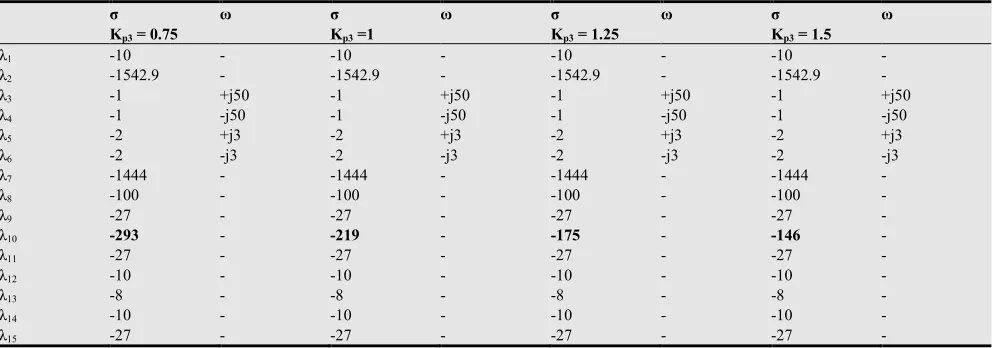
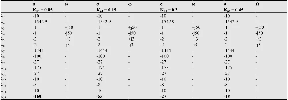
Tables (1- 6) show the effect of changing the values of the proportional controllers coefficients for DFIG on stabil-ity analysis. The coefficients may be ranked depending on its effects on the stability. The most effective proportional coefficient controller is Kp2. This coefficient affects on two

modes of states and made a huge change on the locations of these two poles. The six proportional coefficients may be ranked from the most effective to the least effective de-pending on the changed that they made on the eigenvalues compared to the change on their own values as Kp2, Kp3,

Kp1, Kp4, Kp6, Kp5.

(6)

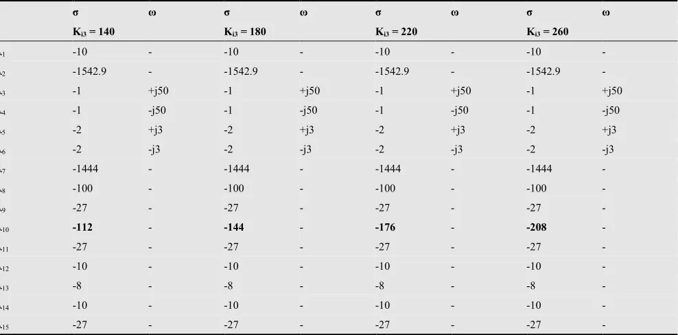
be ranked from the most effective to the least effective de-pending on the changed that they made on the eigenvalues compared to the change on their own values as Ki3, Ki1, Ki2,

Ki4, Ki5, Ki6. Table (13) shows the range of values for the

controllers coefficients for DFIG.

Table 1. Eigenvalues of the DFIG for changing the proportional coefficient value Kp1

σ ω σ ω σ ω σ ω

Kp1 = 0.5 Kp1 = 0.75 Kp1 = 1 Kp1 = 1.25

λ1 -10 - -10 - -10 - -10 -

λ2 -1542.9 - -1542.9 - -1542.9 - -1542.9 -

λ3 -1 +j50 -1 +j50 -1 +j50 -1 +j50

λ4 -1 -j50 -1 -j50 -1 -j50 -1 -j50

λ5 -2 +j3 -2 +j3 -2 +j3 -2 +j3

λ6 -2 -j3 -2 -j3 -2 -j3 -2 -j3

λ7 -1444 - -1444 - -1444 - -1444 -

λ8 -200 - -133 - -100 - -80 -

λ9 -27 - -27 - -27 - -27 -

λ10 -175 - -175 - -175 - -175 -

λ11 -27 - -27 - -27 - -27 -

λ12 -10 - -10 - -10 - -10 -

λ13 -8 - -8 - -8 - -8 -

λ14 -10 - -10 - -10 - -10 -

λ15 -27 - -27 - -27 - -27 -

σ ω σ ω σ ω σ Ω

Kp2 = 0.05 Kp2 = 0.15 Kp2 = 0.3 Kp2 = 0.45

λ1 -10 - -10 - -10 - -10 -

λ2 -1542.9 - -1542.9 - -1542.9 - -1542.9 -

λ3 -1 +j50 -1 +j50 -1 +j50 -1 +j50

λ4 -1 -j50 -1 -j50 -1 -j50 -1 -j50

λ5 -2 +j3 -2 +j3 -2 +j3 -2 +j3

λ6 -2 -j3 -2 -j3 -2 -j3 -2 -j3

λ7 -1444 - -1444 - -1444 - -1444 -

λ8 -100 - -100 - -100 - -100 -

λ9 -160 - -53 - -27 - -18 -

λ10 -175 - -175 - -175 - -175 -

λ11 -160 - -53 - -27 - -18 -

λ12 -10 - -10 - -10 - -10 -

λ13 -8 - -8 - -8 - -8 -

λ14 -10 - -10 - -10 - -10 -

λ15 -27 - -27 - -27 - -27 -

Kp3 = 0.75 Kp3 =1 Kp3 = 1.25 Kp3 = 1.5

λ1 -10 - -10 - -10 - -10 -

λ2 -1542.9 - -1542.9 - -1542.9 - -1542.9 -

λ3 -1 +j50 -1 +j50 -1 +j50 -1 +j50

λ4 -1 -j50 -1 -j50 -1 -j50 -1 -j50

λ5 -2 +j3 -2 +j3 -2 +j3 -2 +j3

λ6 -2 -j3 -2 -j3 -2 -j3 -2 -j3

λ7 -1444 - -1444 - -1444 - -1444 -

λ8 -100 - -100 - -100 - -100 -

λ9 -27 - -27 - -27 - -27 -

λ10 -293 - -219 - -175 - -146 -

λ11 -27 - -27 - -27 - -27 -

λ12 -10 - -10 - -10 - -10 -

λ13 -8 - -8 - -8 - -8 -

λ14 -10 - -10 - -10 - -10 -

(7)

Kp4 = 0.05 Kp4 = 0.15 Kp4 = 0.3 Kp4 = 0.45

λ1 -10 - -10 - -10 - -10 -

λ2 -1542.9 - -1542.9 - -1542.9 - -1542.9 -

λ3 -1 +j50 -1 +j50 -1 +j50 -1 +j50

λ4 -1 -j50 -1 -j50 -1 -j50 -1 -j50

λ5 -2 +j3 -2 +j3 -2 +j3 -2 +j3

λ6 -2 -j3 -2 -j3 -2 -j3 -2 -j3

λ7 -1444 - -1444 - -1444 - -1444 -

λ8 -100 - -100 - -100 - -100 -

λ9 -27 - -27 - -27 - -27 -

λ10 -175 - -175 - -175 - -175 -

λ11 -27 - -27 - -27 - -27 -

λ12 -10 - -10 - -10 - -10 -

λ13 -8 - -8 - -8 - -8 -

λ14 -10 - -10 - -10 - -10 -

λ15 -160 - -53 - -27 - -18 -

Kp5 = 5 Kp5 =7.5 Kp5 = 10 Kp5 =12.5

λ1 -10 - -10 - -10 - -10 -

λ2 -1542.9 - -1542.9 - -1542.9 - -1542.9 -

λ3 -1 +j50 -1 +j50 -1 +j50 -1 +j50

λ4 -1 -j50 -1 -j50 -1 -j50 -1 -j50

λ5 -2 +j3 -2 +j3 -2 +j3 -2 +j3

λ6 -2 -j3 -2 -j3 -2 -j3 -2 -j3

λ7 -1444 - -1444 - -1444 - -1444 -

λ8 -100 - -100 - -100 - -100 -

λ9 -27 - -27 - -27 - -27 -

λ10 -175 - -175 - -175 - -175 -

λ11 -27 - -27 - -27 - -27 -

λ12 -20 - -13 - -10 - -8 -

λ13 -8 - -8 - -8 - -8 -

λ14 -20 - -13 - -10 - -8 -

λ15 -27 - -27 - -27 - -27 -

Kp6= 5 Kp6 = 10 Kp6 = 15 Kp6 = 20

λ1 -10 - -10 - -10 - -10 -

λ2 -1542.9 - -1542.9 - -1542.9 - -1542.9 -

λ3 -1 +j50 -1 +j50 -1 +j50 -1 +j50

λ4 -1 -j50 -1 -j50 -1 -j50 -1 -j50

λ5 -2 +j3 -2 +j3 -2 +j3 -2 +j3

λ6 -2 -j3 -2 -j3 -2 -j3 -2 -j3

λ7 -1444 - -1444 - -1444 - -1444 -

λ8 -100 - -100 - -100 - -100 -

λ9 -27 - -27 - -27 - -27 -

λ10 -175 - -175 - -175 - -175 -

λ11 -27 - -27 - -27 - -27 -

λ12 -10 - -10 - -10 - -10 -

λ13 -24 - -12 - -8 - -6 -

λ14 -10 - -10 - -10 - -10 -

(8)

Table 7. Eigenvalues of the DFIG for changing the integral coefficient value Ki1

Ki1 = 50 Ki1 = 75 Ki1 = 100 Ki1 = 125

λ1 -10 - -10 - -10 - -10 -

λ2 -1542.9 - -1542.9 - -1542.9 - -1542.9 -

λ3 -1 +j50 -1 +j50 -1 +j50 -1 +j50

λ4 -1 -j50 -1 -j50 -1 -j50 -1 -j50

λ5 -2 +j3 -2 +j3 -2 +j3 -2 +j3

λ6 -2 -j3 -2 -j3 -2 -j3 -2 -j3

λ7 -1444 - -1444 - -1444 - -1444 -

λ8 -50 - -75 - -100 - -125 -

λ9 -27 - -27 - -27 - -27 -

λ10 -175 - -175 - -175 - -175 -

λ11 -27 - -27 - -27 - -27 -

λ12 -10 - -10 - -10 - -10 -

λ13 -8 - -8 - -8 - -8 -

λ14 -10 - -10 - -10 - -10 -

λ15 -27 - -27 - -27 - -27 -

Ki2 = 4 Ki2 = 6 Ki2 = 8 Ki2= 10

λ1 -10 - -10 - -10 - -10 -

λ2 -1542.9 - -1542.9 - -1542.9 - -1542.9 -

λ3 -1 +j50 -1 +j50 -1 +j50 -1 +j50

λ4 -1 -j50 -1 -j50 -1 -j50 -1 -j50

λ5 -2 +j3 -2 +j3 -2 +j3 -2 +j3

λ6 -2 -j3 -2 -j3 -2 -j3 -2 -j3

λ7 -1444 - -1444 - -1444 - -1444 -

λ8 -100 - -100 - -100 - -100 -

λ9 -13 - -20 - -27 - -33 -

λ10 -175 - -175 - -175 - -175 -

λ11 -27 - -27 - -27 - -27 -

λ12 -13 - -20 - -27 - -33 -

λ13 -8 - -8 - -8 - -8 -

λ14 -10 - -10 - -10 - -10 -

λ15 -27 - -27 - -27 - -27 -

Ki3 = 140 Ki3 = 180 Ki3 = 220 Ki3 = 260

λ1 -10 - -10 - -10 - -10 -

λ2 -1542.9 - -1542.9 - -1542.9 - -1542.9 -

λ3 -1 +j50 -1 +j50 -1 +j50 -1 +j50

λ4 -1 -j50 -1 -j50 -1 -j50 -1 -j50

λ5 -2 +j3 -2 +j3 -2 +j3 -2 +j3

λ6 -2 -j3 -2 -j3 -2 -j3 -2 -j3

λ7 -1444 - -1444 - -1444 - -1444 -

λ8 -100 - -100 - -100 - -100 -

λ9 -27 - -27 - -27 - -27 -

λ10 -112 - -144 - -176 - -208 -

λ11 -27 - -27 - -27 - -27 -

λ12 -10 - -10 - -10 - -10 -

λ13 -8 - -8 - -8 - -8 -

λ14 -10 - -10 - -10 - -10 -

(9)

Ki4= 4 Ki4 = 6 Ki4 = 8 Ki4 = 10

λ1 -10 - -10 - -10 - -10 -

λ2 -1542.9 - -1542.9 - -1542.9 - -1542.9 -

λ3 -1 +j50 -1 +j50 -1 +j50 -1 +j50

λ4 -1 -j50 -1 -j50 -1 -j50 -1 -j50

λ5 -2 +j3 -2 +j3 -2 +j3 -2 +j3

λ6 -2 -j3 -2 -j3 -2 -j3 -2 -j3

λ7 -1444 - -1444 - -1444 - -1444 -

λ8 -100 - -100 - -100 - -100 -

λ9 -27 - -27 - -27 - -27 -

λ10 -175 - -175 - -175 - -175 -

λ11 -13 - -20 - -27 - -33 -

λ12 -10 - -10 - -10 - -10 -

λ13 -8 - -8 - -8 - -8 -

λ14 -10 - -10 - -10 - -10 -

λ15 -27 - -27 - -27 - -27 -

Ki5 = 50 Ki5= 75 Ki5 = 100 Ki5 = 125

λ1 -10 - -10 - -10 - -10 -

λ2 -1542.9 - -1542.9 - -1542.9 - -1542.9 -

λ3 -1 +j50 -1 +j50 -1 +j50 -1 +j50

λ4 -1 -j50 -1 -j50 -1 -j50 -1 -j50

λ5 -2 +j3 -2 +j3 -2 +j3 -2 +j3

λ6 -2 -j3 -2 -j3 -2 -j3 -2 -j3

λ7 -1444 - -1444 - -1444 - -1444 -

λ8 -100 - -100 - -100 - -100 -

λ9 -27 - -27 - -27 - -27 -

λ10 -175 - -175 - -175 - -175 -

λ11 -27 - -27 - -27 - -27 -

λ12 -5 - -7 - -10 - -13 -

λ13 -8 - -8 - -8 - -8 -

λ14 -5 - -7 - -10 - -13 -

λ15 -27 - -27 - -27 - -27 -

Ki6= 80 Ki6=100 Ki6= 120 Ki6 = 140

λ1 -10 - -10 - -10 - -10 -

λ2 -1542.9 - -1542.9 - -1542.9 - -1542.9 -

λ3 -1 +j50 -1 +j50 -1 +j50 -1 +j50

λ4 -1 -j50 -1 -j50 -1 -j50 -1 -j50

λ5 -2 +j3 -2 +j3 -2 +j3 -2 +j3

λ6 -2 -j3 -2 -j3 -2 -j3 -2 -j3

λ7 -1444 - -1444 - -1444 - -1444 -

λ8 -100 - -100 - -100 - -100 -

λ9 -27 - -27 - -27 - -27 -

λ10 -175 - -175 - -175 - -175 -

λ11 -27 - -27 - -27 - -27 -

λ12 -10 - -10 - -10 - -10 -

λ13 -5 - -7 - -8 - -9 -

λ14 -10 - -10 - -10 - -10 -

λ15 -27 - -27 - -27 - -27 -

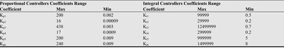
Table 13. The preferred range of values for the controllers coefficients for DFIG for the stability of the system.

Proportional Controllers Coefficients Range Integral Controllers Coefficients Range

Coefficient Max Min Coefficient Max Min

Kp1 200 0.002 Ki1 99999 0.5

Kp2 16 0.00009 Ki2 29999 0.2

Kp3 438 0.003 Ki3 12499999 0.7

Kp4 17 0.0009 Ki4 299999 0.2

Kp5 200 0.009 Ki5 999999 5

(10)

7. Effect of Changing the Generator

Parameters on the Stability

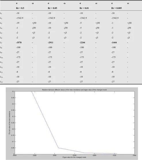
As the value of the resistance or inductance changes the stability degree will change. In this section we will try to find the relation between the increasing or decreasing these

values and the stability degree. Table (14) shows different values of the resistance and the corresponding eigenvalues. Figure (5) shows the relation between different values of the rotor resistance and the eigenvalues of the changed. From Figures (5) we conclude that as the resistance value of the rotor increase, the stability degree will increase.

Table 14. Eigenvalues of DFIG for different values of resistance.

Rr = 0.5 Rr = 0.05 Rr = 0.01 Rr = 0.005

λ1 -10 - -10 - -10 - -10 -

λ2 -1542.9 - -1542.9 - -1542.9 - -1542.9 -

λ3 -19 +j50 -10 +j50 -5 +j50 -1 +j50

λ4 -1 -j50 -10 -j50 -5 -j50 -1 -j50

λ5 -2 +j3 -2 +j3 -2 +j3 -2 +j3

λ6 -2 -j3 -2 -j3 -2 -j3 -2 -j3

λ7 -3578 - -2911 - -2244 - -1444 -

λ8 -100 - -100 - -100 - -100 -

λ9 -27 - -27 - -27 - -27 -

λ10 -175 - -175 - -175 - -175 -

λ11 -27 - -27 - -27 - -27 -

λ12 -10 - -10 - -10 - -10 -

λ13 -8 - -8 - -8 - -8 -

λ14 -10 - -10 - -10 - -10 -

λ15 -27 - -27 - -27 - -27 -

(11)

Table 15. Eigenvalues of DFIG for different values of inductance.

σ ω σ Ω σ ω σ ω

Ls = 0.01 Ls = 0.1 Ls = 1 Ls = 2

λ1 -10 - -10 - -10 - -10 -

λ2 -1542.9 - -1542.9 - -1542.9 - -1542.9 -

λ3 -1 +j50 -1 +j50 -1 +j50 -1 +j50

λ4 -1 -j50 -1 -j50 -1 -j50 -1 -j50

λ5 -2 +j3 -2 +j3 -2 +j3 -2 +j3

λ6 -2 -j3 -2 -j3 -2 -j3 -2 -j3

λ7 -1822 - -1750 - -1556 - -1444 -

λ8 -100 - -100 - -100 - -100 -

λ9 -27 - -27 - -27 - -27 -

λ10 -175 - -175 - -175 - -175 -

λ11 -27 - -27 - -27 - -27 -

λ12 -10 - -10 - -10 - -10 -

λ13 -8 - -8 - -8 - -8 -

λ14 -10 - -10 - -10 - -10 -

λ15 -27 - -27 - -27 - -27 -

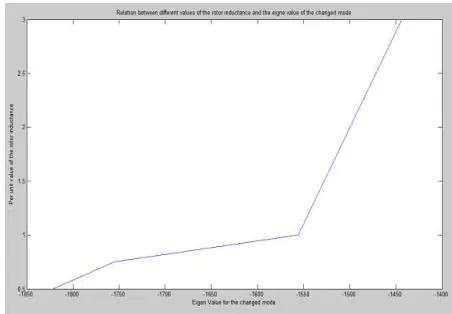
Table (15) shows different values of the inductance and the corresponding eigenvalues for DFIG. Figure (6) shows the relation between different values of the rotor induc-tance and the eigenvalues of the changed mode in case of DFIG. From Figures (9) we conclude that as the inductance value increase as the stability will decrease because of in-creasing the delay time.

Figure 6. The relation between different values of the rotor inductance and the eigenvalues of the changed mode in case of DFIG.

8. Conclusion

The use of tidal currents as a renewable source of energy is very effective as it relies on the same technologies used in offshore wind generation and it is a more predictable source of energy. The overall dynamic system of the tidal current turbine for a single machine infinite bus system and the controllers used for improving the power system sta-bility has been modeled. The equations for a small signal stability analysis for the generator has been formulated. Tidal current turbines without controllers do have the capa-bility to sustain a small disturbance for a long period but it is more beneficial to use PI controllers with the tidal cur-rent turbines to improve system stability. As the value of the coefficients of the PI controllers change, the stability degree will change. For DFIG the most effective propor-tional coefficient controller is Kp2 and the most effective

integral coefficient controller is Ki3. The preferred ranges

of the controllers coefficients values for the system stabili-ty are concluded in this work. As the resistance value in-creases, the stability degree will increase but the system efficiency will decrease. On the contrary, as the inductance value of the machine increases, the stability degree will decrease. The future work will be focused on the optimal values for these coefficients to enhance the system stability.

Appendix

Tidal current turbine parameters

R=18 m, Rs= 0.01 pu, Cp=0.46, Vtide=4 m/s,Ht=3 s, Hg= 0.5 s, Ks=0.171, Kpt=10, Kit=100, Ks= 10 pu, Ds= 3.14 pu.

Generator parameters

Lm=2.9pu, Lr=0.156 pu, Ls=0.171 pu, Rr=0.005pu.

Converter parameters

VDC=1.5 pu, C=0.0001 pu.

Controller parameters

Kp1=1 pu, Kp2=0.3 pu, Kp3=1.25 pu, Kp4=0.3 pu, Kp5=10 pu, Kp6=15 pu, Ki1=100 s-1, Ki2=8 s-1, Ki3=219 s-1, Ki4=8 s-1, Ki5=100 s-1, Ki6=120 s-1.

Hamed H. H. Aly received the B.Sc. and M.Sc. degrees in electrical engineering with distinction, in 1999 and 2005, respectively, from Zagazig University, Egypt and the Ph.D. degree from Dalhousie University, Halifax, NS, Canada, in 2012. His research interests include Forecasting, Modeling, Control, power system quality, integration of the renewable energy into the electrical grid, Smart Grid and power sys-tem stability. Dr. Aly is currently doing his postdoctoral fellowship and working as an instructor at Dalhousie Uni-versity in the Faculty of Engineering and the Faculty of Science.

M. E. El-Hawary (S’68–M’72–F’90) received the

(12)

1968 and the Ph.D. degree from the University of Alberta, Edmonton, AB, Canada, in 1972. He was a Killam Me-morial Fellow at the University of Alberta. He is now a Professor of electrical and computer engineering at Dalh-ousie University, Halifax, NS, Canada. He served on the faculty and was a Chair of the Electrical Engineering De-partment at Memorial University of Newfoundland for eight years. He was an Associate Professor of electrical engineering at the Federal University of Rio de Janeiro, Rio de Janeiro, Brazil, for two years and was an Instructor at the University of Alexandria. He pioneered many com-putational and artificial intelligence solutions to problems in economic/environmental operation of power systems. He has written ten textbooks and monographs and more than 122 refereed journal articles. He has consulted and taught for more than 42 years.

Dr. El-Hawary is a Fellow of the Engineering Institute of Canada (EIC) and the Canadian Academy of Engineering (CAE).

References

[1] ”Tidal Stream” Available online (January 2011), http://www.tidalstream.co.uk/html/background.html [2] ”Tidal Currents” Available online (April 2011),

http://science.howstuffworks.com/environmental/earth/ocea nography/ocean-current4.htm

[3] Hamed H. H. Aly, and M. E. El-Hawary “State of the Art for Tidal Currents Electrical Energy Resources”, 24th An-nual Canadian IEEE Conference on Electrical and Com-puter Engineering, Niagara Falls, Ontario, Canada, 2011. [4] Hamed H. Aly, and M. E. El-Hawary “An Overview of

Offshore Wind Electrical Energy Systems” 23rd Annual Ca-nadian IEEE Conference on Electrical and Computer Engi-neering, Calgary, Alberta, Canada, May 2-5, 2010.

[5] Marcus V. A. Nunes, J. A. Peças Lopes, Hans Helmut, Ubi-ratan H. Bezerra, and Rogério G. “Influence of the Variable-Speed Wind Generators in Transient Stability Margin of the Conventional Generators Integrated in Electrical Grids” IEEE Transactions on Energy Conversion, 2004.

[6] J.G. Slootweg, H.Polinder and W.L. Kling“Dynamic Mod-eling of a Wind Turbine with Doubly Fed Induction

Genera-tor” IEEE Power Engineering Society Summer Meeting, 2001.

[7] Janaka B. Ekanayake, Lee Holdsworth, XueGuang Wu, and Nicholas Jenkins” Dynamic Modeling of Doubly Fed In-duction Generator Wind Turbines” IEEE Transactions on Power Systems, Vol. 18, No. 2, May 2003.

[8] M.J.Khan, G. Bhuyan, A. Moshref, K. Morison, “An As-sessment of Variable Characteristics of the Pacific North-west Regions Wave and Tidal Current Power Resources, and their Interaction with Electricity Demand & Implica-tions for Large Scale Development Scenarios for the Re-gion,” Tech. Rep. 17485-21-00 (Rep 3), Jan. 2008.

[9] Lucian Mihet-Popa, Frede Blaabjerg, and Ion Boldea,” Wind Turbine Generator Modeling and Simulation Where Rotational Speed is the Controlled Variable” IEEE Transac-tions On Industry ApplicaTransac-tions, Vol. 58, No. 1, Janu-ary/February 2004.

[10] Seif Eddine Ben Elghali, Rémi Balme, Karine Le Saux, Mohamed El Hachemi Benbouzid, Jean Frédéric Charpen-tier, and Frédéric Hauville “A Simulation Model for the Evaluation of the Electrical Power Potential Harnessed by a Marine Current Turbine” IEEE Journal of Ocean Engineer-ing, October 2007.

[11] Hamed H. H. Aly, and M. E. El-Hawary, “Small Signal Stability Analysis of Tidal In-Stream Turbine Using DDPMSG with and without Controller” IEEE Annual Elec-trical Power and Energy Conference, Winnipeg, Canada, 2011.

[12] Yazhou Lei, Alan Mullane, Gordon Lightbody, and Robert Yacamini “Modeling of the Wind Turbine with a Doubly Fed Induction Generator for Grid Integration Studies” IEEE Transaction on Energy Conversion, Vol. 28, No. 1, March 2006.

[13] F. Wu, X.-P. Zhang, and P. Ju “Small signal stability analy-sis and control of the wind turbine with the direct-drive permanent magnet generator integrated to the grid” Journal of Electric Power and Engineering Research, 2009. [14] F. Wu, X.-P. Zhang, and P. Ju “Small signal stability

analy-sis and optimal control of a wind turbine with doubly fed induction generator” IET Journal of Generation, Transmis-sion and Distribution, 2007.