Active Imitation Learning: Formal and Practical Reductions
to I.I.D. Learning
Kshitij Judah [email protected]
Alan P. Fern [email protected]
Thomas G. Dietterich [email protected]
Prasad Tadepalli [email protected]
School of Electrical Engineering and Computer Science Oregon State University
1148 Kelley Engineering Center Corvallis, OR 97331-5501, USA
Editor:Joelle Pineau
Abstract
In standard passive imitation learning, the goal is to learn a policy that performs as well as a target policy by passively observing full execution trajectories of it. Unfortunately, generating such trajectories can require substantial expert effort and be impractical in some cases. In this paper, we consideractive imitation learning with the goal of reducing this effort by querying the expert about the desired action at individual states, which are selected based on answers to past queries and the learner’s interactions with an environment simulator. We introduce a new approach based on reducing active imitation learning to active i.i.d. learning, which can leverage progress in the i.i.d. setting. Our first contribution is to analyze reductions for both non-stationary and stationary policies, showing for the first time that the label complexity (number of queries) of active imitation learning can be less than that of passive learning. Our second contribution is to introduce a practical algorithm inspired by the reductions, which is shown to be highly effective in five test domains compared to a number of alternatives.
Keywords: imitation learning, active learning, active imitation learning, reductions
1. Introduction
Traditionally, passive imitation learning involves learning a policy that performs nearly as well as an expert’s policy based on a set of trajectories of that policy. However, generating such trajectories is often tedious or even impractical for an expert (e.g., real-time low-level control of multiple game agents). In order to address this issue, we consider active imitation learning where full trajectories are not required, but rather the learner asks queries about specific states, which the expert labels with the correct actions. The goal is to learn a policy that is nearly as good as the expert’s policy using as few queries as possible.
The active learning problem for i.i.d. supervised learning1 has received considerable
attention both in theory and in practice (Settles, 2012), which motivates leveraging that
work for active imitation learning. However, the direct application of i.i.d. approaches to active imitation learning can be problematic. This is because active i.i.d. learning algorithms assume access to either a target distribution over unlabeled input data (in our case states) or a large sample drawn from it. The goal then is to select the most informative query to ask, usually based on some combination of label (in our case actions) uncertainty and unlabeled data density. Unfortunately, in active imitation learning, the learner does not have direct access to the target state distribution, which is the state distribution induced by the unknown expert policy.
In principle, one could approach active imitation learning by assuming a uniform or an arbitrary distribution over the state space and then apply an existing active i.i.d. learner. However, such an approach can perform very poorly. This is because if the assumed dis-tribution is considerably different from that of the expert, then the learner is prone to ask queries in states rarely or even never visited by the expert. For example, consider a bicycle balancing problem. Clearly, asking queries in states where the bicycle has entered an un-avoidable fall is not very useful, because no action can prevent a crash. However, an active i.i.d. learning technique will tend to query in such uninformative states, leading to poor performance, as shown in our experiments. Furthermore, in the case of a human expert, a large number of such queries poses serious usability issues, since labeling such states is clearly wasted effort from the expert’s perspective.
In this paper, we consider the problem of reducing active imitation learning to active i.i.d. learning both in theory and practice. Our first contribution is to analyze the Probably Approximately Correct2 (PAC) label complexity (number of expert queries) of a reduction for learning non-stationary policies, which requires only minor modification to existing results for passive learning. Our second contribution is to introduce a reduction for learning stationary policies resulting in a new algorithm,Reduction-based Active Imitation Learning
(RAIL), and an analysis of the label complexity. The resulting complexities for active
imitation learning are expressed in terms of the label complexity for the i.i.d. case and show that there can be significant query savings compared to existing results for passive imitation learning. Our third contribution is to describe a new practical algorithm, RAIL-DA (for data aggregation), inspired by the RAIL algorithm, which makes a series of calls to an active i.i.d. learning algorithm. We evaluate RAIL-DA in five test domains and show that it is highly effective when used with an i.i.d. algorithm that takes the unlabeled data density into account.
The rest of the paper is organized as follows. We begin by reviewing the relevant related work in Section 2. In Section 3, we present the necessary background material and describe the active imitation learning problem setup. In Section 4, we present the proposed reductions for the cases of non-stationary and stationary policies. In Section 5, we present the RAIL-DA algorithm. In Section 6, experimental results are presented. In Section 7, we summarize and present some directions for future research.
2. Related Work
Active learning has been studied extensively in the i.i.d. supervised learning setting (Settles, 2012) but to a much lesser degree for sequential decision making, which is the focus of
active imitation learning. Several studies have considered active learning forreinforcement
learning (RL) (Clouse, 1996; Mihalkova and Mooney, 2006; Gil et al., 2009; Doshi et al.,
2008), where learning is based on both autonomous exploration and queries to an expert. In our imitation learning framework, in contrast, we do not assume a reward signal and learn only from expert queries. Other work (Shon et al., 2007) studies active imitation learning in a multiagent setting, where the expert is itself a reward seeking agent which acts to maximize its own reward, and hence is not necessarily helpful for learning. In the current setting, we only consider helpful experts.
One approach to imitation learning isinverse RL (IRL) (Ng and Russell, 2000), where a reward function is learned based on a set of target policy trajectories. The learned reward function and transition dynamics are then given to a planner to obtain a policy. There has been limited work on active IRL. This includes Active Sampling (Lopes et al., 2009), a Bayesian approach where the posterior over reward functions is used to select the state with maximum uncertainty over the actions. Another Bayesian approach (Cohn et al., 2010, 2011) models uncertainty about the entire MDP model and uses a decision-theoretic criterion, Expected Myopic Gain (EMG), to select various types of queries to pose to the expert, e.g., queries about transition dynamics, the reward function, or optimal action at a particular state. For autonomous navigation tasks, Silver proposed two active IRL techniques that request demonstrations from the expert on examples that are either novel (novelty reduction) or uncertain (uncertainty reduction) to the learner (Silver et al., 2012). Specifically, in novelty reduction, a start and goal location is selected such that the path that may most likely be demonstrated by the expert results in the learner seeing novel portions of the navigation terrain. This helps in learning behavior on previously unseen regions of the navigation terrain. In uncertainty reduction, a start and goal location is selected such that there is high uncertainty about the best path from start to goal.
While promising, the scalability of these approaches is hindered by the assumptions made by IRL, and these approaches have only been demonstrated on small problems. In particular, they require that the exact domain dynamics are provided or can be learned, which is often not realistic, for example, in the Wargus domain considered in this paper. Furthermore, even when a model is available, prior IRL approaches require an efficient planner for the MDP model. For the large domains considered in this paper, standard planning techniques for flat MDPs, which scale polynomially in the number of states, are not practical. While there has been substantial work on MDP planning for large domains via the use of factored representations (e.g., Boutilier et al. 1999) or simulators (e.g., Kocsis and Szepesvri 2006), robustness and scalability are still problematic in general.
To facilitate scalability, rather than following an IRL framework we consider a direct
imitation framework where we attempt to directly learn a policy instead of the reward
Active learning work in the direct imitation framework includes Confidence Based Au-tonomy (CBA) (Chernova and Veloso, 2009), and the related dogged learning framework (Grollman and Jenkins, 2007), where a policy is learned in an online manner as it is exe-cuted. When the learner is uncertain about what to do at the current state, the policy is paused and the expert is queried about what action to take, resulting in a policy update. The execution resumes from the current state with the learner taking the action suggested by the expert. One can roughly view CBA as a reduction of imitation learning to stream-based active learning where the learner receives unlabeled inputs (states) one at a time and must decide whether or not to request the label (action) of the current input. CBA makes this decision by estimating its uncertainty about the action to take at a given state and requesting an action label for states with uncertainty above a threshold. One difficulty in applying this approach is setting the uncertainty threshold for querying the expert. While an automated threshold selection approach is suggested by Chernova and Veloso (Chernova and Veloso, 2009), our experiments show that it is not always effective (See Section 6). In particular, we observed that the proposed threshold selection mechanism is quite sensitive to the initial training data supplied to the learner.
Recently, Ross et al. proposed novel algorithms for imitation learning that are able to actively query the expert on states encountered during the execution of the policy being trained (Ross and Bagnell, 2010; Ross et al., 2011). The motivation behind these algo-rithms is to eliminate the discrepancy between the training (expert’s) and test (learner’s) state distributions that arises in the traditional passive imitation learning approach when-ever the learned policy is unable to exactly mimic the expert’s policy. This discrepancy often leads to the poor performance of the traditional approach. Note that such an issue is not present in the i.i.d. learning setting, where mistakes made by the learner do not in-fluence the distribution of future test samples. They show that under certain assumptions their algorithms achieve better theoretical performance guarantees than traditional passive imitation learning.
However, because the primary goal of these algorithms is not to minimize the labeling effort of the expert, these algorithms query the expert quite aggressively, which makes them impractical for human experts or computationally expensive with automated experts. To see this, consider the first iteration of the DAGGER algorithm proposed by Ross et al. (Ross et al., 2011). In the first iteration, DAGGER trains a policy on a set of expert-generated trajectories, as in passive imitation learning. Thus, in practice the query complexity of the first iteration of DAGGER will be similar to that of passive imitation learning. In subsequent iterations, additional queries are asked by querying the expert on states along trajectories produced by learned policies in prior iterations. In contrast, our work focuses on active querying for the purpose of minimizing the expert’s labeling effort. In particular, we show that an active approach can achieve an improved query complexity over passive in theory (under certain assumptions) and in practice. Like our work, their approach also requires a dynamics simulator to help select queries.
(Khardon, 1999). He showed that for any policy class for which there exists a consistent learner, the class is efficiently learnable in the sense that only a polynomial number of expert trajectories are required by the learner to produce a policy as good as the expert’s policy. However, the result holds for only deterministic policies in the realizable setting and the generalizations to stochastic policies and the agnostic setting were left as future work.
More recently, Syed and Schapire performed theoretical analysis of passive imitation learning in a more general setting where the expert policy is allowed to be stochastic and the learning can be agnostic (Syed and Schapire, 2010). In their analysis, they take a reduction based approach, where the problem of passive imitation learning is reduced to classification, and they relate the performance of the learned policy to the accuracy of the classifier. Standard PAC analysis can then be used to show that only a polynomial number of expert trajectories are required to achieve the desired level of performance. A similar analysis was done by Ross and Bagnell (Ross and Bagnell, 2010). To our knowledge, no prior work has addressed the relative sample complexity of active versus passive imitation learning, which is one of the primary contributions of this paper. Some of the material in this paper appeared in an earlier version of the paper (Judah et al., 2012).
3. Problem Setup and Background
In this section, we present the necessary background material and formally set up the active imitation learning problem.
3.1 Markov Decision Processes
We consider imitation learning in the framework of Markov decision processes (MDPs). An MDP is a tuple hS, A, P, R, Ii, where S is the set of states, A is the finite set of actions,
P(s, a, s0) is the transition function denoting the probability of transitioning to state s0
upon taking actionain states,R(s, a)∈[0,1] is the reward function giving the immediate reward in statesupon taking action a, and I is the initial state distribution. A stationary policyπ:S 7→Ais a deterministic mapping from states to actions such thatπ(s) indicates the action to take in state s when executing π. A non-stationary policy is a tuple π = (π1, . . . , πT) of T stationary policies such thatπ(s, t) =πt(s) indicates the action to take in
statesat timetwhen executingπ, whereT is the time horizon. The expert’s policy, which we assume is deterministic, is denoted byπ∗.
A key concept used in this paper is the notion of a state distribution of a policy at a particular time step. We usedtπ :S 7→[0,1] to denote the state distribution induced at time step t by starting in s1 ∼I and then executing π. Note that d1π =I for all policies. We
usedπ = T1 PT
t=1dtπ to denote the state distribution induced by policyπ overT time steps.
To sample an (s, a) pair from dtπ, we start in s1 ∼ I, execute π to generate a trajectory
T = (s1, a1, . . . , sT, aT, sT+1) and set (s, a) = (st, at). Similarly, to sample fromdπ, we first
sample a random time step t ∈ {1, . . . , T}, and then sample an (s, a) pair from dtπ. Note that in order to sample from dπ∗ (or dtπ∗), we need to execute π∗. Throughout the paper,
The T-horizon value of a policy V(π) is the expected total reward of trajectories that start ins1 ∼I at timet= 1 and then executeπ forT steps. This can be expressed as
V(π) =T ·Es∼dπ[R(s, π(s))].
The regret of a policyπ with respect to an expert policyπ∗ is equal to V(π∗)−V(π).
3.2 Problem Setup
Passive Imitation Learning. In imitation learning, the goal is to learn a policy π with a
small regret with respect to the expert. In this work, we consider the direct imitation learn-ing settlearn-ing, where the learner directly selects a policy π from a hypothesis class Π (e.g., linear action classifiers). In thepassive imitation learning setup, the protocol is to provide the learner with a training set of full execution trajectories ofπ∗ and the state-action pairs (or a sample of them) are passed to a passive i.i.d. supervised learning algorithm Lp. The hypothesis π∈Π that is returned byLp is used as the learned policy.
Active Imitation Learning. To help avoid the cost of generating full trajectories, the active
imitation learning setup allows the learner to pose action queries. Each action query
in-volves presenting a state sto the expert and then obtaining the desired action π∗(s) from the expert. In addition to having access to the expert for answering queries, we assume that the learner has access to a simulator of the MDP. The input to the simulator is a policyπ
and a horizon T. The simulator output is a state trajectory that results from executing π
forT steps starting in the initial state. The learner is allowed to interact with this simulator as part of its query selection process. The simulator is not assumed to provide a reward signal, which means that the learner cannot find π by pure reinforcement learning. The only way for the learner to gain information about the target policy is through queries to the expert at selected states.
Given access to the expert and the simulator of the MDP, the goal in active imitation learning is to learn a policy π ∈ Π that has a small regret by posing as few queries to the expert as possible. Note that it is straightforward for the active learner to generate full expert trajectories by querying the expert at each state of the simulator it encounters. Thus, an important baseline active learning approach is to generate an appropriate number
N of expert trajectories for consumption by a passive learner. The number of queries for this baseline isN·T. A fundamental question that we seek to address is whether an active learner can achieve the same performance with significantly fewer queries both in theory and in practice.
3.3 Background on I.I.D. Learning
Since our analysis in the next two sections is based on reducing to active i.i.d. learning and comparing to passive i.i.d. learning, we briefly review the Probably Approximately Correct
(PAC) (Valiant, 1984) learning formulation for the i.i.d. setting. Here we consider the
re-alizable PAC setting, which will be the focus of our initial analysis. Section 4.3 extends to the non-realizable or agnostic setting.
from an unknown distribution DX over an input space X and are labeled according to an
unknown target classifierf :X 7→ Y, whereY denotes the label space. In the realizable PAC setting it is assumed thatf is an element of a known class of classifiersHand, given a set of
N examples, a learner outputs a hypothesis h ∈H. Let ef(h, DX) =Ex∼DX[h(x) 6=f(x)]
denote the generalization error of the returned classifier h. Standard PAC learning theory provides a bound on the number of labeled examples that is sufficient to guarantee that for any distribution DX, with probability at least 1−δ, the returned classifier h will satisfy ef(h, DX)≤. We will denote this bound byNp(, δ), which corresponds to the label/query
complexity of i.i.d. passive supervised learning for a class H. We will also denote a passive learner that achieves this label complexity asLp(, δ).
Active Learning. In active i.i.d. learning, the learner is given access to two resources rather
than just a set of training data: 1) A “cheap” resource (Sample) that can draw an unlabeled sample fromDX and provide it to the learner when requested, 2) An “expensive” resource
(Label) that can label a given unlabeled sample according to target concept f when re-quested. Given access to these two resources, an active learning algorithm is required to learn a hypothesis h∈H while posing as few queries to Label as possible. It can, however, pose a much larger number of queries to Sample (though still polynomial), as it is cheap.
Unlike passive i.i.d. learning, formal label/query complexity results for active i.i.d. learn-ing depend not only on the hypothesis class belearn-ing considered, but also on joint properties of the target hypothesis and data distribution (e.g., as measured by the disagreement co-efficient proposed by Hanneke, 2009). We use Na(, δ, DX) to denote the label complexity
(i.e., calls to Label) that is sufficient for an active learner to return an h that for distri-bution DX with probability at least 1−δ satisfies ef(h, DX) ≤. Note that here we did
not explicitly parameterizeNaby the target hypothesisf since, in the context of our work,
f will correspond to the expert policy and can be considered as fixed. We will denote an active learner that achieves this label complexity as La(, δ, D), where the final argument Dindicates that the Sample function used by La samples from distributionD.
It has been shown that for certain problem classes,Nacan be exponentially smaller than Np (Hanneke, 2009; Dasgupta, 2011). For example, in the realizable learning setting (i.e., the target concept is in the hypothesis space), for any active learning problem with finite VC-dimension and finite disagreement coefficient, the sample complexity is exponentially smaller for active learning compared to passive learning with respect to 1. That is, ignoring the dependence on δ, Np = O(1) whereas Na =O(log(1)). A concrete problem for which this is the case is when the data are uniformly distributed on a unit sphere in addimensional input spaceRd, and the hypothesis spaceH consists of homogeneous linear separators. As
an example active learning algorithm that achieves this performance, the algorithm of Cohn et al. (Cohn et al., 1994) simply samples a sequence of unlabeled examples and queries for the label of example x only when there are at least two hypotheses that disagree on the label ofx, but agree on all previously labeled examples.
asymptotically improve over passive learning across all problems with finite VC-dimension. However, despite the limited theoretical understanding, there is much empirical evidence that in practice active learning algorithms can often dramatically reduce the required amount of labeled data compared to passive learning. Further, there are active learning algorithms that in the worst case are guaranteed to achieve performance similar to passive learning in the worst case, while also showing exponential improvement in the best case (Beygelzimer et al., 2009a).3
4. Reductions for Active Imitation Learning
One approach to solving novel machine learning problems is via reduction to well-studied core problems. A key advantage of this reduction approach is that theoretical and empir-ical advances on the core problems can be translated to the more complex problem. For example, i.i.d. multi-class and cost-sensitive classification have been reduced to i.i.d. binary classification (Zadrozny et al., 2003; Beygelzimer et al., 2009b). In particular, these reduc-tions allow guarantees regarding binary classification to translate to the target problems. Further, the reduction-based algorithms have shown equal or better empirical performance compared to specialized algorithms. More closely related to our work, in the context of sequential decision making, both imitation learning and structured prediction have been re-duced to i.i.d. classification (Daum´e et al., 2009; Syed and Schapire, 2010; Ross and Bagnell, 2010).
In this section, we consider a reduction approach to active imitation learning. In par-ticular, we reduce to active i.i.d. learning, which is a core problem that has been the focus of much theoretical and empirical work. The key result is to relate the label complexity of active imitation learning to the label complexity of active i.i.d. learning. In doing so, we can assess when improved label complexity (either empirical or theoretical) of active i.i.d. learning over passive i.i.d. learning can translate to improved label complexity of active imi-tation learning over passive imiimi-tation learning. In what follows, we first present a reduction for the case of deterministic non-stationary policies. Next, we give a reduction for the more difficult case of deterministic stationary policies.
4.1 Non-Stationary Policies
Syed and Schapire analyze the traditional reduction from passive imitation learning to passive i.i.d. learning for non-stationary policies (Syed and Schapire, 2010). The algorithm receives N expert trajectories as input, noting that the state-action pairs at time t across trajectories can be viewed as i.i.d. draws from distributiondtπ∗. The algorithm, then returns
the non-stationary policy ˆπ = (ˆπ1, . . . ,πˆT), where ˆπt is the policy returned by running the
learner Lp on examples from time t.
Let t = eπ∗
t(ˆπt, d
t
π∗) be the generalization error of ˆπt at time t. Syed and Schapire
(Syed and Schapire, 2010, Lemma 3)4 show that if at each time step t ≤0, then V(ˆπ)≥
V(π∗)−0T2. Hence, if we are interested in learning a ˆπwhose regret is no more thanwith high probability, then we must simultaneously guarantee that with high probabilityt≤ T2 at all time steps. This can be achieved by calling the passive learner Lp at each time step withNp(T2,Tδ) examples. Thus, the overall passive label complexity of this algorithm (i.e., the number of actions provided by the expert) isT ·Np(T2,Tδ). To our knowledge, this is the best known label complexity for passive imitation learning of non-stationary policies.
Our goal now is to provide a reduction from active imitation learning to active i.i.d. learning that can achieve an improved label complexity. A naive way to do this would simply replace calls to Lp in the above approach with calls to an active learner La. Note,
however, that in order to do this the active learner at time step t requires the ability to sample from the unlabeled distributiondtπ∗. Generating each such unlabeled sample requires
executing the expert policy fort steps from the initial state, which in turn requirest label queries to the expert. Thus, the label complexity of this naive approach will be at least linearly related to the number of unlabeled examples required by the active i.i.d. learning algorithm. Typically, this number is similar to the passive label complexity rather than the potentially much smaller active label complexity. Thus, the naive reduction does not yield an advantage over passive imitation learning.
It turns out that for a slightly more sophisticated reduction to passive i.i.d. learning, introduced by Ross and Bagnell (Ross and Bagnell, 2010), it is possible to simply replaceLp
withLaand maintain the potential benefit of active learning. Ross and Bagnell introduced
the forward training algorithm for non-stationary policies, which trains a non-stationary policy in a series of T iterations. In particular, iteration t trains policy ˆπt by calling a passive learnerLp on a labeled data set drawn from the state distribution induced at time t by the non-stationary policy ˆπt−1 = (ˆπ
1, . . . ,πˆt−1), where ˆπ1 is learned on states drawn
from the initial distribution I. The motivation for this approach is to train the policy at time steptbased on the same state-distribution that it will encounter when being run after learning. By doing this, they show that the algorithm has a worst case regret of T2 and
under certain assumptions can achieve a regret as low as O(T).
Importantly, the state-distribution used to train ˆπtgiven bydtπˆt−1 is easy for the learner to sample from without making queries to the expert. In particular, to generate a sample the learner can simply simulate ˆπt−1, which is available from previous iterations, from a random initial state and return the state at timet. Thus, we can simply replace the call to
Lp at iteration t with a call to La with unlabeled state distribution dtˆπt−1 as input. More formally, theactive forward training algorithm is presented in Algorithm 1.
Ross and Bagnell (Ross and Bagnell, 2010, Theorem 3.1) give the worst case bound on the regret of the forward training algorithm which assumes the generalization error at each iteration is bounded by. Since we also maintain that assumption when replacingLp with
La (the active variant) we immediately inherit that bound.
Algorithm 1 Active Forward Training
Input: active i.i.d. learning algorithm La, ,δ Output: non-stationary policy ˆπ = (ˆπ1, . . . ,πˆT)
1: Initialize ˆπ1 =La(,Tδ, I) .queries by La answered by expert; unlabeled data
is generated from initial state distributionI. 2: for t = 2 toT do
3: πˆt−1 = (ˆπ1, . . . ,πˆt−1)
4: πˆt =La(,Tδ, dπtˆt−1) . queries byLa answered by expert; unlabeled data is
generated using simulator and ˆπt−1 as described in the main text.
5: end for
6: return πˆ= (ˆπ1, ...,πˆT)
Proposition 1 Given a PAC active i.i.d. learning algorithm La, if active forward training
is run by giving La parameters and Tδ at each step, then with probability at least 1−δ it
will return a non-stationary policy ˆπ such that V(ˆπ)≥V(π∗)−T2.
Note that La is run with Tδ as the reliability parameter to ensure that all T iterations
succeed with probability at least 1−δ.
We can apply Proposition 1 to obtain the overall label complexity of active forward training required to achieve a regret of less than with probability at least 1−δ. In particular, we must run the active learner at each of the T iterations with parameters T2 and Tδ, giving an overall label complexity ofPT
t=1Na(T2,Tδ, dπtˆt−1), whered1πˆ0 =I and the ˆ
πt−1 are random variables in this expression. Recall, from above, that the best known label complexity of passive imitation learning is T·Np(T2,Tδ).
Comparing these quantities we see that if we use an active learning algorithm whose sample complexity is no worse than that of passive, i.e., Na(T2,Tδ, dtπˆt−1) is no worse than
Np(T2,Tδ) for any t, then the expected sample complexity of active imitation learning will be no worse than the passive case. As mentioned in the previous section, such i.i.d. active learning algorithms can be realized. Further, if in addition, for some iterations the expected value ofNa(T2,Tδ, dtˆπt−1) for some values oftis better than the passive complexity, then there will be an overall expected improvement over passive imitation learning. While this additional condition cannot be verified in general, we know that such cases can exist, including cases of exponential improvement. Further, empirical experience in the i.i.d. setting also suggests that in practiceNa can often be expected to be substantially smaller thanNp and rarely worse. The above result suggests that those empirical gains will be able
to transfer to the imitation learning setting.
4.2 Stationary Policies
A drawback of active forward training is that it is impractical for largeT and the resulting policy cannot be run indefinitely. We now consider the case of learning stationary policies; first we review the existing results for passive imitation learning.
In the traditional approach, a stationary policy ˆπ is trained on the expert state distribu-tiondπ∗using a passive learning algorithmLp and returning a stationary policy ˆπ. Ross and
Algorithm 2 RAIL
Input: active i.i.d. learning algorithm La, ,δ Output: stationary policy ˆπ
1: Initialize ˆπ0 to arbitrary policy or based on prior knowledge 2: for t = 1 toT do
3: πˆt=La(, δ
T, dˆπt−1) . queries by La answered by expert; unlabeled data is
generated using simulator as described in Section 3 4: end for
5: return πˆT
with respect to the i.i.d. distributiondπ∗ is bounded by0 thenV(ˆπ)≥V(π∗)−0T2. Since
generating i.i.d. samples from dπ∗ can require up to T queries (see Section 3) the passive
label complexity of this approach for guaranteeing a regret less than with probability at least 1−δ isT·Np(T2, δ). Again, to our knowledge, this is the best known label complexity for passive imitation learning. Further, Ross and Bagnell (Ross and Bagnell, 2010) show that there are imitation learning problems where this bound is tight, showing that in the worst case, the traditional approach cannot be shown to do better.
The above approach cannot be converted into an active imitation learner by simply re-placing the call toLp withLa, since again we cannot sample from the unlabeled distribution
dπ∗ without querying the expert. To address this issue, we introduce a new algorithm called
RAIL (Reduction-based Active Imitation Learning) which makes a sequence of T calls to
an active i.i.d. learner, noting that it is likely to find a useful stationary policy well before all T calls are issued. RAIL is an idealized algorithm intended for analysis, which achieves the theoretical goals but has a number of inefficiencies from a practical perspective. Later in Section 5, we describe the practical instantiation that is used in our experiments.
RAIL is similar in spirit to active forward training, though its analysis is quite different and more involved. Like forward-training, RAIL iterates for T iterations, but on each iteration, RAIL learns a new stationary policy ˆπt that can be applied across all time steps
t = 1. . . T. Note that T denotes the length of the horizon as well as the total number of iterations that RAIL runs for. Similarly t denotes a single time step as well as a single iteration of RAIL. Iterationt+ 1 of RAIL learns a new policy ˆπt+1 that achieves a low error
rate at predicting the expert’s actions with respect to the state distribution of the previous policydˆπt. More formally, Algorithm 2 gives pseudocode for RAIL. The initial policy ˆπ0 is arbitrary and could be based on prior knowledge and the algorithm returns the final policy ˆ
The complication faced by RAIL, however, compared to forward training, is that the distribution used to train ˆπt+1 differs from the state distribution of the expert policydπ∗.
This is particularly true in early iterations of RAIL, since ˆπ0 is initialized arbitrarily. Intu-itively, however, we might expect that as the iterations proceed, the unlabeled distributions used for training dπt will become similar to dπ∗. To see this, consider the first iteration.
While dπˆ0 need not be at all similar to dπ∗ overall, we know that they will agree on the
initial state distribution. That is, we have that d1πˆ0 =d1π∗ =I. Because of this, the policy
ˆ
π1 learned on dπˆ0 can be expected to agree with the expert on the first step. This implies that the states encountered after the first action of the expert and learned policy will tend to be similar. That is d2πˆ1 will be similar tod2π∗. In this same fashion we might expectdt+1πˆt to be similar todt+1π∗ after iterationt. We now show that this intuition can be formalized in
order to bound the disparity betweendπˆT anddπ∗, which will allow us to bound the regret
of the learned policy. We first state the main result, which we prove below.
Theorem 2 Given a PAC active i.i.d. learning algorithmLa, if RAIL is run with
parame-tersand Tδ passed toLaat each iteration, then with probability at least 1−δ it will return
a stationary policy πˆ such that V(ˆπ)≥V(π∗)−T3.
Recall that the corresponding regret for active forward training of non-stationary policies was T2. From this we see that the impact of moving from non-stationary to stationary policies in the worst case is a factor of T in the regret bound. Similarly the bound is a factor of T worse than the comparable result above for passive imitation learning, which suffered a worst-case regret of T2. From this we see that the total label complexity for RAIL required to guarantee a regret of with probability 1−δ is PT
t=1Na(
T3,Tδ, dπˆt−1) compared to the above label complexity of passive learning T·Np(T2, δ).
We first compare these quantities in the worst case. If, in each iteration, the active i.i.d. label complexity is the same as the passive complexity, then active imitation learning via RAIL can ask more queries than passive. That is, the active complexity would scale as
T ·Np(T3,Tδ) versusT ·Np(T2, δ), which is dominated by the factor of T1 difference in the accuracy parameters. In the realizable setting with finite VC-dimension, RAIL’s complexity could be a factor ofT higher than passive in this worst-case scenario.
However, if across the iterations the expected active i.i.d. label complexityNa(T3,Tδ, dπˆt−1) is substantially better than Np(T3,Tδ), then RAIL will leverage those savings. For exam-ple, in the realizable setting with finite VC-dimension, if all distributionsdπˆt−1 result in a finite disagreement coefficient, then we can get exponential savings. In particular, ignor-ing the dependence on δ (which is only logarithmic), we get an active label complexity of
O(TlogT3) versus the corresponding passive complexity of O(T3).
The above analysis points to an interesting open problem. Is there an active imitation learning algorithm that can guarantee to never perform worse than passive, while at the same time showing exponential improvement in the best case?
state two lemmas, that are useful for the final proof. First, we bound the regret of a policy in terms ofPπT(M).
Lemma 3 For any policy π, ifPT
π(M)≥1−, then V(π)≥V(π∗)−T.
Proof Let Γ∗ and Γ be all state-action sequences of length T that are consistent with π∗
and π respectively. If R(T) is the total reward for a sequenceT then we get the following
V(π) = X
T ∈Γ
Pr(T |M, π)R(T)
≥ X
T ∈Γ∩Γ∗
Pr(T |M, π)R(T)
= X
T ∈Γ∗
Pr(T |M, π∗)R(T)− X
T ∈Γ∗−Γ
Pr(T |M, π∗)R(T)
= V(π∗)− X
T ∈Γ∗−Γ
Pr(T |M, π∗)R(T)
≥ V(π∗)−T · X
T ∈Γ∗−Γ
Pr(T |M, π∗)
≥ V(π∗)−T.
The last two inequalities follow since the reward for a sequence must be no more than T, and due to our assumption aboutPπT(M).
Next, we show how the value of Pπt(M) changes across one iteration of RAIL. We show that if we learn a policy ˆπ on state distribution dπ(M) of policy π whose error rate
eπ∗(ˆπ, dπ(M)) (see Section 3.3) w.r.t. to the expert’s policy π∗ is no more than , then Pˆπt+1(M) is at least as large as Pπt(M)−T . Whenπ and ˆπ correspond to policies learned at iterationtand (t+ 1) respectively, then Lemma 4 describes change in the value ofPπt(M) across one iteration.
Lemma 4 For any policies π andπˆ and 1≤t < T, ifeπ∗(ˆπ, dπ(M))≤, thenPt+1 ˆ
π (M)≥ Pπt(M)−T .
Proof We define ˆΓ to be all sequences of state-action pairs of lengtht+1 that are consistent with ˆπ. Also define Γ to be all length t+ 1 state-action sequences that are consistent with
π on the first t state-action pairs (so need not be consistent on the final pair). We also define M0 to be an MDP that is identical to M, except that the transition distribution of any state-action pair (s, a) is equal to the transition distribution of action π(s) in state s. That is, all actions taken in a state sbehave like the action selected byπ ins.
We start by arguing that ifeπ∗(ˆπ, dπ(M))≤thenPt+1 ˆ π (M
0)≥1−T , which relates our
error assumption to the MDPM0. To see this, note that for MDPM0, all policies, including
π∗, have state distribution given bydπ. Thus by the union bound 1−Pπˆt+1(M0)≤Pt+1
i=1i,
sinceeπ∗(ˆπ, dπ(M)) = 1 T
PT
i=1i. Using this fact we can now derive the following
Pπˆt+1(M) = X
T ∈Γˆ
Pr(T |M, π∗)
≥ X
T ∈Γ∩Γˆ
Pr(T |M, π∗)
= X
T ∈Γ
Pr(T |M, π∗)− X
T ∈Γ−Γˆ
Pr(T |M, π∗)
= Pπt(M)− X
T ∈Γ−ˆΓ
Pr(T |M, π∗)
= Pπt(M)− X
T ∈Γ−ˆΓ
Pr(T |M0, π∗)
≥ Pπt(M)−X
T 6∈Γˆ
Pr(T |M0, π∗)
≥ Pπt(M)−(1−Pπˆt+1(M0)) ≥ Pπt(M)−T .
The equality of the fourth line follows because Γ contains all sequences whose firsttactions are consistent withπwith all possible combinations of the remaining action and state tran-sition. Thus, summing over all such sequences yields the probability thatπ∗ agrees with the first tsteps. The equality of the fifth line follows because Pr(T |M, π∗) = Pr(T |M0, π∗) for any T that is in Γ and for which π∗ is consistent (has non-zero probability underπ∗). The final line follows from the above observation thatPˆπt+1(M0)≥1−T .
We can now complete the proof of the main theorem.
Proof [Proof of Theorem 2] Using failure parameter Tδ in the call toLa in each iteration of RAIL ensures that with at least probability (1−δ) that for all 1≤t≤T, we will have
eπ∗(ˆπt, dπˆt−1(M))≤, wheredπˆ0(M) denotes the state distribution of the initial policy ˆπ0. This can be easily shown using the union bound. Next, we show using induction that for 1≤t≤T, we havePπˆtt ≥1−tT . As a base case for iterationt= 1, we havePπˆ11 ≥1−T , since the the error rate of ˆπ1 relative to the initial state distribution at time step t= 1 is at most T (this is the worst case when all errors are committed at time step 1). Assume that the inequality holds for t=k, i.e.,Pˆπkk ≥1−kT . Consider ˆπk+1 trained ondˆπk(M). By the union bound argument above, we know that eπ∗(ˆπk+1, dπˆk(M))≤ . Hence, ˆπk+1 and ˆπk satisfy the precondition of Lemma 4. Therefore we have
Pπˆk+1k+1 ≥ P
k ˆ
πk−T (by Lemma 4)
≥ 1−kT −T (by inductive argument)
≥ 1−(k+ 1)T .
Hence, for 1 ≤ t ≤ T, we have Pπˆtt ≥ 1−tT . In particular, when t = T, we have
4.3 Agnostic Case
Above we considered the realizable setting, where the expert’s policy was assumed to be in a known hypothesis classH. In the agnostic case, we do not make such an assumption. The learner still outputs a hypothesis from a classH, but the unknown policy is not necessarily inH. The agnostic i.i.d. PAC learning setting is defined similarly to the realizable setting, except that rather than achieving a specified error bound ofwith high probability, a learner must guarantee an error bound of infπ∈Hef(π, DX)+with high probability (wheref is the
target), whereDX is the unknown data distribution. That is, the learner is able to achieve
close to the best possible accuracy given class H. In the agnostic case, it has been shown that exponential improvement in label complexity with respect to 1 is achievable when infπ∈Hef(π, DX) is relatively small compared to (Dasgupta, 2011). Further, there are
many empirical results for practical active learning algorithms that demonstrate improved label complexity compared to passive learning.
It is straightforward to extend our above results for non-stationary and stationary poli-cies to the agnostic case by using agnostic PAC learners for Lp and La. Here we outline
the extension for RAIL. Note that the RAIL algorithm will call La using a sequence of
unlabeled data distributions, where each distribution is of the form dπ for some π ∈ H
and each of which may yield a different minimum error given H. For this purpose, we define ∗ = supπ∈Hinfπˆ∈Heπ∗(ˆπ, dπ) to be the minimum generalization error achievable
in the worst case considering all possible state distributions dπ that RAIL might possibly encounter. With minimal changes to the proof of Theorem 1, we can get an identical result, except that the regret is (∗+)T3 rather than just T3. A similar change in regret holds for passive imitation learning. This shows that in the agnostic setting we can get significant improvements in label complexity via active imitation learning when there are significant savings in the i.i.d. case.
5. RAIL-DA: A Practical Variant of RAIL
Despite the theoretical guarantees, there are at least two potential drawbacks of the RAIL algorithm from a practical perspective. First, RAIL does not share labeled data across iterations which is potentially wasteful in practice, though important for our analysis. In practice, we might expect that aggregating labeled data across iterations would be beneficial due to the larger amount of data. This is somewhat confirmed by the empirical success of the DAGGER algorithm (Ross et al., 2011) and motivates evaluating the use of data aggregation within RAIL. Incorporating data aggregation into RAIL, however, complicates the theoretical analysis, which we leave for future work. The second practical inefficiency of RAIL is that the unlabeled state distributions used at early iterations may be quite different fromdπ∗. In particular, the state distribution of policy ˆπt, which is used to train the policy
Algorithm 3 RAIL+
Input: L0,n,AccumData,N,K . L0 : initial set of labeled data
. n : no. of queries per iteration
. AccumData : accumulate data across iterations or not
. N : committee size for DWQBC
. K : # trajectories used to generate unlabeled data Output: stationary policy ˆπ
1: Initialize L=L0
2: whilequery budget remaining do
3: U =SampleUnlabeledData(K,L) .generates pool of unlabeled data
4: if !AccumData then 5: Initialize L=L0
6: end if
7: for i= 1 to ndo . selectn queries from poolU
8: s=DWQBC(L,U,N) . density-weighted QBC is used as active i.i.d. learner
9: L=L∪ {(s,Label(s))} . obtain label from expert
10: end for
11: end while
12: return ˆπ =SupervisedLearn(L)
We now describe a parameterized practical instantiation of RAIL used in our experi-ments, which is intended to address the above issues and also specify certain other imple-mentation details. Algorithm 3 gives pseudocode for this algorithm, which we call RAIL+ to distinguish it from the idealized version of RAIL in our analysis. In Section 6, we will compare different instances of RAIL+, including parameterizations corresponding to pure RAIL and RAIL-DA (for data aggregation), which is the primary algorithm in our empirical study. We note that our description assumes the use of a pool-based active learner, which is a common active learning setting, meaning that the learner requires as input a pool of unlabeled examples U that represents the unlabeled target distribution.
5.1 Data Aggregation and Incremental Querying
The first major difference compared to RAIL is that RAIL+ can aggregate data across iterations when the Boolean parameter AccumData is set to true. In this case, during each iteration the newly labeled data is added to the set of labeled data from previous iterations (lines 7-10). Otherwise, the labeled data from previous iterations is discarded after generating unlabeled dataU (lines 4-6).
The second major difference is that RAIL+ may ask fewer queries per iteration than RAIL as specified by the parameter n. RAIL corresponds to a version of RAIL+ that does not use data aggregation and has n = Na. Because RAIL+ can aggregates data, it
Algorithm 4 Density-Weighted Query-By-Committee Algorithm
1: procedure DWQBC(L,U,N)
2: C =SampleCommittee(N,L) . committee represents posterior over policies
3: dˆL=EstimateDensity(U) . estimate density of states inU (see text)
4: s∗ = argmax{V E(s, C)∗dˆL(s) :s∈U} .selection heuristic (see text)
5: return s∗
6: end procedure
(lines 2-11). Each iteration starts with the current set of labeled examples L, which have been accumulated across all previous iterations by RAIL+. This set of examples is used to generate a pool U of unlabeled examples/states (see details below) intended to represent the unlabeled target distribution. A pool-based active learner, DWQBC (explained later), is then calledntimes to selectnqueries from this pool. Each query is labeled by the expert and added to the growing set of labeled training data L. After the n queries have been issued andL is updated, the next iteration begins.
This incremental version of RAIL allows for rapid updating of the unlabeled state dis-tributions used for learning (represented via U) and prevents RAIL from using its query budget on earlier less accurate distributions. In our experiments, we find that using n= 1 is most effective compared to larger values, which facilitates the most rapid update of the distribution. In this case, each query selected by the active i.i.d. learner is based on the most up-to-date state distribution, which takes all prior data into account. We refer to this best performing variant of RAIL+ with n= 1 and data aggregation as RAIL-DA.
An interesting variation to RAIL+is when queries take a non-trivial amount of real-time to answer and there arekexperts available that can answer queries in parallel. In this case, it can be beneficial to askksimultaneous queries per iteration in order to reduce the amount of real-time required to learn a policy. The problem of selecting ksuch queries is known as
batch active learning, and a variety of approaches are available for the i.i.d. setting (Brinker,
2003; Xu et al., 2007; Hoi et al., 2006a,b; Guo and Schuurmans, 2008; Azimi et al., 2012). An advantage of our reduction-based approach to active imitation learning is that we can directly plug in the i.i.d. batch active learner in our framework without requiring any other changes to be made.
5.2 Density Weighted QBC
Algorithm 5 Procedure SampleUnlabeledData
1: procedure SampleUnlabeledData(K,L)
2: C =SampleCommittee(K,L) . committee represents posterior over policies
3: U ={} .initialize multi-set of unlabeled data
4: for π∈C do
5: S= SimulateTrajectory(π) . states generated on trajectory ofπ
6: U =U∪S
7: end for
8: return U
9: end procedure
Intuitively, the selection heuristic of DWQBC attempts to trade off the uncertainty about what to do at a state (measured by VE) with the likelihood that the state is relevant to learning the target policy (measured by the density).
5.3 Bayesian Learner
The final choice we make while implementing RAIL+ (and hence RAIL-DA) is again mo-tivated by the goal of arriving at an accurate unlabeled data distribution as quickly as possible. Recall that at iteration t+ 1, RAIL learns using an unlabeled data distribution
dˆπt, where ˆπt is a point estimate of the policy based on the labeled data from iteration t. In order to help improve the accuracy of this unlabeled distribution (with respect to dπ∗),
instead of using a point estimate, we adopt a Bayesian approach in RAIL+. In particular,
at iteration t let L be the set of state-action pairs collected from the previous iteration (or from all previous iterations if data is accumulated). We use this to define a posterior
P(ˆπ|L) over policies in our policy class H. This distribution, in turn, defines a posterior unlabeled state distribution dL =Eπˆ∼P(ˆπ|L)[dˆπ(s)] that RAIL+ effectively uses in place of dˆπt as used in RAIL. Note that we can sample states fromdL by first sampling a policy ˆπ and then sampling a state fromdπˆ, all of which can be done without interaction with the
expert.
Our implementation of this idea uses bootstrap aggregation (Breiman, 1996) in order to approximate dL by an unlabeled data pool U via a call to the procedure Sample-UnlabeledData in Algorithm 3 (line 3). Our implementation assumes a class of linear parametric policies with a zero-mean Gaussian prior over the parameters. The procedure first uses bootstrap aggregation to approximate sampling a set of policies from the posterior (Algorithm 5, line 2) forming a “committee” C of K policies. We view C as an empirical distribution representing the posterior over policies. In particular, each policy is the result of first generating a bootstrap sample of the current labeled data and then calling a super-vised learner on the sampled data. Each member of the committee is then simulated to form a state trajectory, and the states on those trajectories are aggregated to produce the unlabeled data pool U (Algorithm 5, lines 4-7). Our implementation uses K = 5.
Algorithm 6 Procedure SampleCommittee
1: procedure SampleCommittee(K,L) 2: C ={} . initialize the committee 3: for i= 1 to K do
4: L0 =BootstrapSample(L) .create a bootstrap sample of L
5: π0 =SupervisedLearn(L0) .learn a classifier(policy) using L0
6: C=C∪π0
7: end for
8: return C
9: end procedure
In practice, dL is a significantly more useful estimate of dπ∗ than the point estimate
with respect to learning a policy. This is because it places more weight on states that are more frequently visited by policies drawn from the posterior rather than just a single policy. As an extreme example of the advantage of usingdL in practice, consider active imitation learning in an MDP with deterministic dynamics and a single start state. At iteration t, RAIL will use the state distribution of the point estimate ˆπt−1, which for our assumed
MDP will be uniform over the deterministic state sequence generated by ˆπt−1. Thus, active learning will place equal emphasis on learning among that set of states. This is despite the fact that, in early iterations, we should expect that states appearing later in the trajectory are less likely to be relevant to learning π∗. This is because inaccuracies in ˆπt−1 lead to error propagation as the trajectory unfolds. In contrast, dL will weigh states according to
the trajectories produced by all policies, weighted by the posterior. The practical effect is a non-uniform distribution over states in those trajectories, roughly weighted by how many policies visit the states. Thus, states at the tail end of trajectories in early iterations will generally carry very little weight, since they are only visited by one or a small number of policies.
6. Experiments
compare it with a number of baseline approaches to active imitation learning in our last set of experiments. Finally, we provide some overall observations.
For all the learners in the experiments that are presented in this section, we employed the SimpleLogistic classifier from Weka (Hall et al., 2009) to learn policies over the set of features that were provided for each domain.
6.1 Domain Details
In this subsection, we give the details of all the domains used in our experiments.
6.1.1 Cart-Pole
Cart-pole is a well-known RL benchmark. In this domain, there is a cart on which rests a vertical pole. The objective is to keep the attached pole balanced by applying left or right force to the cart. An episode ends when either the pole falls or the cart goes out of bounds. There are two actions, left and right, and four state variables (x,x, θ,˙ θ˙) describing the position and velocity of the cart and the angle and angular velocity of the pole. We made slight modifications to the usual setting where we allow the pole to fall down and become horizontal and the cart to go out of bounds (we used [-2.4, 2.4] as the in bounds region). We let each episode run for a fixed length of 5000 time steps. This opens up the possibility of generating several “undesirable” states where either the pole has fallen or the cart is out of bounds that are rarely or never generated by the expert’s state distribution.
For all the experiments in cart-pole, the learner’s policy is represented via a linear logistic regression classifier using features of state-action pairs where features correspond to state variables. The expert policy was a hand-coded policy that can balance the pole indefinitely. For each learner, we ran experiments from 150 random initial states close to the equilibrium start state ((x,x, θ,˙ θ˙) = (0.0,0.0,0.0,0.0)). For each start state a policy is learned and a learning curve is generated measuring the performance as function of number of queries posed to the expert. To measure performance, we use a reward function (unknown to the learner) that gives +1 reward for each time step where the pole is kept balanced and the cart is within bounds and −1 otherwise. The final learning curve is the average of the individual curves.
6.1.2 Bicycle Balancing
This domain is a variant of the RL benchmark of bicycle balancing and riding (Randløv and Alstrøm, 1998). The goal is to balance a bicycle moving at a constant speed for 1000 time steps. If the bicycle falls, it remains fallen for the rest of the episode. Similar to the cart-pole domain, in bicycle balancing there is a huge possibility of spending significant amount of time in “undesirable” states where the bicycle has fallen down. The state space is described using nine variables (ω,ω, θ,˙ θ, ψ, x˙ f, yf, xb, yb), where ω and ˙ω are the vertical angle and
angular velocity of the bicycle,θand ˙θare the angle and angular velocity of the handlebar,ψ
is the angle of the bicycle to the goal,xf andyf are x and y coordinates of the front tire and
As in the cart-pole domain, for all experiments in bicycle balancing, the learner’s policy is represented as a linear logistic regression classifier over features of state-action pairs. A feature vector for a state-action pair is defined as follows: Given a states, a vector consisting of following 20 basis functions is computed:
(1, ω, ω, ω˙ 2, ω˙2, ωω, θ,˙ θ, θ˙ 2, θ˙2, θθ, ωθ, ωθ˙ 2, ω2θ, ψ, ψ2, ψθ, ψ,¯ ψ¯2, ψθ¯ )T,
where ¯ψ = π−ψ if ψ > 0 and ¯ψ = −π −ψ if ψ < 0. This vector of basis functions is repeated for each of the 5 actions giving a feature vector of length 100. The expert policy was hand-coded and can balance the bicycle for up to 26K time steps. We used a similar evaluation procedure as for cart-pole where we generated 150 random start states and for each start state, a policy was learned using each of the learning algorithms and a learning curve was generated measuring total reward as function of number of queries posed to the expert. We give a +1 reward for each time step where the bicycle is kept balanced and a −1 reward otherwise.
6.1.3 Wargus
We consider controlling a group of 5 friendly close-range military units against a group of 5 enemy units in the real-time strategy game Wargus, similar to the setup used by Judah et al. (Judah et al., 2010). The objective is to win the battle while minimizing the loss in total health of friendly units. The set of actions available to each friendly unit is to attack any one of the remaining units present in the battle (including other friendly units, which is always a bad choice). In our setup, we allow the learner to control one of the units throughout the battle, whereas the other friendly units are controlled by a fixed “reasonably good” policy. This situation would arise when training the group via coordinate ascent on the performance of individual units. The expert policy corresponds to the same policy used by the other units. Note that poor behavior from even a single unit generally results in a huge loss.
The learner’s policy is represented using 27 state-action features that capture different information about the current battle situation such as the distance between the friendly agent and the target of attack, whether the target is already under attack by other friendly units, health of the target relative to friendly unit, whether the target is actually a friendly unit, etc. Providing full demonstrations in real time in such tactical battles is very difficult for human players and quite time consuming if demonstrations are done in slow motion, which motivates state-based active learning for this domain. For experiments, we designed 21 battle maps differing in the initial unit positions, using 5 for training and 16 for testing. We report results in the form of learning curves showing the performance metric as a function of number of queries posed to the expert. We use the difference in the total health of friendly and enemy units at the end of the battle as the performance metric (which is positive for a win). Due to the slow pace of the experiments running on the Wargus infrastructure, we average results across at most 20 trials.
6.1.4 Driving Domain
Figure 1: Screenshot of the driving simulator.
bed used to evaluate the confidence based autonomy (CBA) learner in prior work (Chernova and Veloso, 2009). Here we evaluate RAIL-DA on a particular implementation of the driving domain used by Cohn et al. (Cohn et al., 2011). In this domain, the goal is to successfully navigate a car through traffic on a busy five lane highway. The highway consists of three traffic lanes and two shoulder lanes (see Figure 1). The learner controls the black car, which moves at a constant speed. The other cars move at a randomly chosen continuous-valued constant speed, and they don’t change lanes. At each discrete time step, the learner controls the car by taking one of the three actions: 1)Left, which moves the car to the adjacent left lane, 2)Right, which moves the car to the adjacent right lane, and 3)Stay, which keeps the car in the current lane. The agent is allowed to drive on the shoulder lane but cannot move off the shoulder lanes.
The learner’s policy is represented as a linear logistic regression classifier that maps a given state to one of the three actions. The state space is represented using 68 features. The first 5 features are binary features that specify the learner’s current lane. The next 3 binary features specify whether the learner is colliding with, tailgating or trailing another car. The remaining 60 features, consisting of three parts, one for the learner’s current lane and two for the two adjacent lanes, which are binary features that specify whether the learner’s car will collide with or pass another car in 2X time steps, where X ranges from 0 to 19. This captures the agent’s view of the traffic while taking car velocities into account.
6.1.5 Structured Prediction
We evaluate RAIL-DA on two structured prediction tasks, stress prediction and phoneme prediction, both based on the NETtalk data set (Dietterich et al., 2008). In stress prediction, given a word, the goal is to assign one of the 5 stress labels to each letter of the word in left-to-right order so that the word is pronounced correctly. The output labels are ‘2’ (strong stress), ‘1’ (medium stress), ‘0’ (light stress), ‘<’ (unstressed consonant, center of syllable to the left), and ‘>’ (unstressed consonant, center of syllable to the right). In phoneme prediction, the task is to assign one of the 51 phoneme labels to each letter of the word. It is straightforward to view structured prediction as imitation learning (see for example Ross et al., 2011,Daum´e et al., 2009) where at each time step (letter location), the learner has to execute the correct action (i.e., predict correct label) given the current state. The state consists of features describing the input (the current letter and its immediate neighbors) and the previousLpredictions made by the learner (the prediction context). In our experiments, we useL= 1,2.
The NETtalk data set consists of 2000 words divided into 1000 training words and 1000 test words. Each method is allowed to select a state located on any of the words in the training data and pose it as a query. The expert reveals the correct label at that location. We use character accuracy as a measure of performance. The details of how in each learning trial RAIL-DA and other baselines select a query from the set of training words will be described when we present our results in the following subsections. We report final performance in the form of learning curves averaged across 50 learning trials.
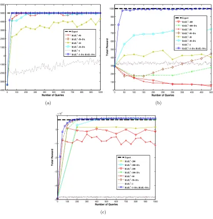
6.2 Experiment 1: Evaluation of the Effects of Data Aggregation and Query Size
We compare different versions of RAIL+, by varying the parametersAccumData and nin Algorithm 3, in order to observe the impact of data aggregation and query size. We use the notationRAIL+-n-DAfor versions that aggregate data and ask nqueries per iteration and
useRAIL+-n to denote variants that askn queries per iteration without data aggregation. Note that RAIL+-1-DA is the same as RAIL-DA and that RAIL+-n with a large value ofn
corresponds to the original version of RAIL from our analysis. Note that all these variants use the DWQBC active i.i.d. learner as described in Section 5.
For this experiment, we focus on three domains: 1) Cart-Pole, 2) Bicycle Balancing, and 3) Driving Domain. In each domain, we evaluated RAIL+-n-DA and RAIL+-n for values of nstarting atn= 1 in increments until some maximum value. The maximum value ofn
in each domain was selected to be a value where i.i.d. active learning from the true expert state distribution reliably converged to a near perfect policy. For each RAIL+ variant and domain, we show the averaged learning curve as described earlier.
0 100 200 300 400 500 600 700 800 900 1000 −4000 −3000 −2000 −1000 0 1000 2000 3000 4000 5000 6000
Number of Queries
Total Reward
Expert RAIL+−50 RAIL+−50−DA RAIL+−10 RAIL+−10−DA RAIL+−1 RAIL+−1−DA (RAIL−DA)
(a)
0 50 100 150 200 250 300 350 400 450 500 0 100 200 300 400 500 600 700 800 900 1000
Number of Queries
Total Reward
Expert RAIL+−100 RAIL+−100−DA RAIL+−50 RAIL+−50−DA RAIL+−10 RAIL+−10−DA RAIL+−1 RAIL+−1−DA (RAIL−DA)
(b)
0 100 200 300 400 500 600 700 800 900 1000 −5 −4 −3 −2 −1 0 1x 10
4
Number of Queries
Total Reward
Expert
RAIL+−200 RAIL+−200−DA RAIL+−100 RAIL+−100−DA RAIL+−50 RAIL+−50−DA RAIL+−1 RAIL+−1−DA (RAIL−DA)
(c)
particularly important for small values of n, such as n = 1 and n = 10, where without aggregation each iteration is learning from only a small amount of data (the small amount of initial data +n).
Now consider the impact of varying n with the use of aggregation in Bicycle. The clear trend is that when aggregation is being used the performance improves significantly as n decreases from n = 100 to n = 1. That is, the more incremental variants of RAIL+ dominate, withn= 1 (i.e. the RAIL-DA algorithm) dominating all others by a large margin. The main reason for this particularly striking trend is that in Bicycle the distributions being learned from in early iterations are quite distant from that of the expert. In particular, the early iterations involve learning from state distributions of policies that result in early crashes, and hence many useless states from the point of view of learning. This means that when using n = 100, the first 100 queries are selected from such a distribution and not much is learned. In fact, we see a downward trend, indicating that learning from those distributions hurts performance. On the other hand, asndecreases fewer queries are spent on those early inaccurate distributions, and the data from a small number of queries per iteration accumulates, resulting in policies that have better state distributions to learn from. Indeed, forn= 1, only one query is asked for each distribution, and we see very rapid improvement until reaching expert performance after just over 50 queries.
Figure 2(a) shows results for Cart-Pole. The target concept in this domain is simpler, and hence the learning curves improve more quickly compared to Bicycle. However, we see the same general trends as for Bicycle. Aggregation is beneficial and we get the best performance for small values ofnwhen using aggregation. Again we see that RAIL+-1-DA (i.e., RAIL-DA) is the top performer. These same trends are observed in Figure 2(c) for Driving.
Overall, these experiments provide strong evidence that in practice aggregation is an important enhancement to RAIL+ over RAIL, and that more incremental variants are preferable. Thus, for the remainder of the paper we will use the RAIL-DA algorithm which uses aggregation and n= 1.
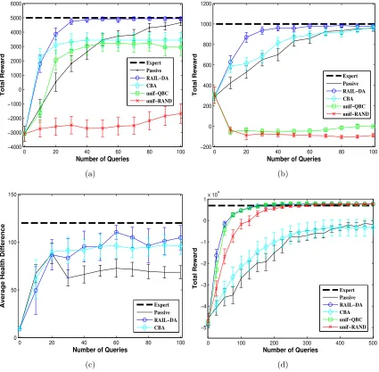
6.3 Experiment 2: Evaluation of RAIL-DA with Different Base Active Learners
In Section 5, we mentioned that it is important that the active i.i.d. learner used with RAIL be sensitive to the unlabeled data distribution. To test this hypothesis, we conducted experiments to study the effects of using active i.i.d. learners that take data distribution into consideration against active learners that ignore the data distribution altogether in RAIL-DA. We compare the performance of three different versions of RAIL-DA: 1)RAIL-DA, the RAIL-DA algorithm from the previous experiment that uses density-weighted QBC as the base active learner, 2)RAIL-DA-QBC, RAIL-DA but with density-weighted QBC replaced with the standard QBC (without density weighting), and 3) RAIL-DA-RAND, which uses random selection of unlabeled data points.
0 10 20 30 40 50 60 70 80 90 100 −4000 −3000 −2000 −1000 0 1000 2000 3000 4000 5000 6000
Number of Queries
Total Reward Expert RAIL−DA RAIL−DA−QBC RAIL−DA−RAND (a)
0 10 20 30 40 50 60 70 80 90 100
−200 0 200 400 600 800 1000 1200
Number of Queries
Total Reward Expert RAIL−DA RAIL−DA−QBC RAIL−DA−RAND (b)
0 10 20 30 40 50 60 70 80 90 100
−20 0 20 40 60 80 100 120 140
Number of Queries
Total Reward Expert RAIL−DA RAIL−DA−QBC RAIL−DA−RAND (c)
0 50 100 150 200 250 300 350 400 450 500
−5 −4 −3 −2 −1 0 1x 10
4
Number of Queries
Total Reward Expert RAIL−DA RAIL−DA−QBC RAIL−DA−RAND (d)
0 50 100 150 200 250 300 0.35
0.4 0.45 0.5 0.55 0.6 0.65 0.7 0.75
Number of Queries
Prediction Accuracy per Character
RAIL−DA RAIL−DA−QBC RAIL−DA−RAND
(a)
0 50 100 150 200 250 300
0.35 0.4 0.45 0.5 0.55 0.6 0.65 0.7 0.75
Number of Queries
Prediction Accuracy per Character
RAIL−DA RAIL−DA−QBC RAIL−DA−RAND
(b)
0 50 100 150 200 250 300
0.1 0.2 0.3 0.4 0.5 0.6 0.7 0.8
Number of Queries
Prediction Accuracy per Character
RAIL−DA RAIL−DA−QBC RAIL−DA−RAND
(c)
0 50 100 150 200 250 300
0.1 0.2 0.3 0.4 0.5 0.6 0.7 0.8
Number of Queries
Prediction Accuracy per Character
RAIL−DA RAIL−DA−QBC RAIL−DA−RAND
(d)
Figure 4: Performance of RAIL-DA with different base active learners on NETtalk: (a) Stress prediction, L = 1 (b) Stress prediction, L = 2 (c) Phoneme prediction,