Consistency and Localizability
Alon Zakai [email protected]
Interdisciplinary Center for Neural Computation Hebrew University of Jerusalem
Jerusalem, Israel 91904
Ya’acov Ritov [email protected]
Department of Statistics
Interdisciplinary Center for Neural Computation and Center for the Study of Rationality Hebrew University of Jerusalem
Jerusalem, Israel 91905
Editor: Gabor Lugosi
Abstract
We show that all consistent learning methods—that is, that asymptotically achieve the lowest pos-sible expected loss for any distribution on(X,Y)—are necessarily localizable, by which we mean that they do not significantly change their response at a particular point when we show them only the part of the training set that is close to that point. This is true in particular for methods that appear to be defined in a non-local manner, such as support vector machines in classification and least-squares estimators in regression. Aside from showing that consistency implies a specific form of localizability, we also show that consistency is logically equivalent to the combination of two properties: (1) a form of localizability, and (2) that the method’s global mean (over the entire X distribution) correctly estimates the true mean. Consistency can therefore be seen as comprised of two aspects, one local and one global.
Keywords: consistency, local learning, regression, classification
1. Introduction
In a supervised learning problem we are given an i.i.d sample Sn={(xi,yi)}i=1..n of size n from
some distribution P; then a new pair(x,y)is drawn from the same P and our goal is to predict y when shown only x. Our prediction (also called estimate, or guess) of y is written f(Sn,x), some
function that depends on the training set and the point at which we estimate (note that it is slightly atypical to have both the training set and point as inputs to f , but this will be very convenient in our setting). We call f a learning method; in the context of regression we will also use the term estimator, and in the context of classification we will use the term classifier. In both of these settings, if f achieves the lowest possible expected loss as n→∞, for every distribution, then we call
f consistent (we will formalize all of these definitions later on; for now we just sketch the general
ideas). Consistent estimators are of obvious interest due to their capability to learn without knowing in advance anything about the actual distribution.
guesses the class of a point x based on its nearest neighbors in the training set, thus, this classifier behaves in a ‘local’ way: only close-by points affect the estimate. More generally, by a locally-behaving method we mean one that, given a training set Sn and a point x at which to estimate
the value of y, in some way treats the close-by part of the training set as the most important. A second type of consistent learning method is defined in a global manner, for example, support vector machines (see Vapnik, 1998; Steinwart, 2002, for a description and proof of consistency, respectively). It is not clear from the definition of support vector machines whether they behave locally or not: The separating hyperplane is determined based on the entire training set Sn, and
furthermore does not depend on the specific point x at which we classify, perhaps leading us to expect that support vector machines do not behave locally. Thus, on an intuitive level we might think that some consistent methods behave locally and some do not.
This intuition also appears relevant when we consider regression: The k-NN regression estima-tor appears to behave locally, while on the other hand support vecestima-tor regression (see, e.g., Smola and Schoelkopf, 1998), kernel ridge regression (Saunders et al., 1998), etc., seem not to have that property. Another example is that of orthogonal series estimation, that is, of using a weighted sum of fixed harmonic functions (Lugosi and Zeger, 1995); this method appears to not behave locally both because the harmonic functions are non-local and because the coefficients are determined in a way based on all of the data.
Despite the intuition that some consistent methods might not behave locally, we will see that in fact all of them necessarily behave in that manner. As mentioned before, we already know that some locally-behaving methods are consistent, since some are in fact defined in a local manner, for example, k-NN. What we will see is that all other consistent methods must also behave locally. In classification, this implies that, in particular, (properly regularized) support vector machines and boosting (Freund and Schapire, 1999; Zhang, 2004; Bartlett and Traskin, 2007) must behave locally, despite being defined in a way that appears global. In the area of regression, our results show that neural network estimators, orthogonal series estimators, etc., must behave locally if they are consistent, again, despite their being defined in a way that does not indicate such behavior.
In the rest of this introductory section we will present a summary of our approach and results as well as background regarding related work. While doing so we focus on regression problems since that setting allows for simpler and clearer definitions. For the same reasons we will also focus on regression in the main part of this paper; in a later section we will show how to apply our results to classification.
Our goal in regression is to estimate f∗(x) =E(y|x), that is, the expected value of y conditioned on x, or the regression of y on x. Our hope is that f(Sn,x) is close to f∗(x). We say that f is
consistent on a distribution P iff
Ln(f)≡E|f(Sn,x)−f∗(x)|−→ n→∞0
where the expected value is taken over training sets Snand observations x both distributed according
to P (which is suppressed in the notation). If a method is consistent on all P then we call it consistent (this is sometimes called universal consistency). Note that there are stronger notions of consistency, such as requiring that the loss converge to 0 with probability 1 (see, e.g., Gyorfi et al., 2002), but we will focus on the loss as just described. Note also that the Lnloss is ‘global’ in that we average over
The notion of local behavior that we will consider will be called localizability, and it entails that the method returns a similar estimate for x when shown Snin comparison to the estimate it would
have returned when shown only the part of Snthat is close to x. In other words, if we define
Sn(x,r) ={(xi,yi)∈Sn : ||xi−x|| ≤r}
then a localizable method has the property that
f(Sn,x)≈ f(Sn(x,r),x)
for some small r>0 (the formal definitions of all of these concepts will be given in later sections). More specifically, for any sequence Rnց0 we can see g(Sn,x) = f Sn x,Rn
,xas a ‘localization’ of f , since it applies f to the close-by part of the training set for the particular point at which we estimate. In other words, a localizable method is one that behaves similarly to a localization of itself. (Note the convenience of the f(Sn,x)notation here, that is, of seeing f as a function of both
Snand x.)
Why is the concept of localizability of interest? The main motivation for us is that, as we will see later, consistency implies a form of localizability. That is, even an estimator defined in what seems to be a global manner, for example, by minimizing a global loss of the general form
1
ni=
∑
1..nl f(xi),yi
+λc(f)
where l is, for example, least-squares, and c is (optional) complexity penalization—then even such an estimator must be in some sense localizable, if it is consistent. Thus, our first motivation is to point out that not only locally-defined methods like k-NN behave locally, but also all other consistent methods as well.
Aside from this main motivation for investigating localizability, another reason is that it allows us to answer questions such as, “What might happen if we localize a support vector machine?” That is, we can apply a support vector machine (or some other useful method) to only the close-by part of the training set, perhaps motivated close-by the fact that training on this smaller set is more computationally efficient, at least if all we need is to generate estimates at a small number of points. If support vector machines are localizable, then we in fact know that such an approach can be consistent; and if they are not localizable, then we may end up with a non-consistent method with poor performance. Thus, localizability can have practical applications.
Note that one can consider other ways to define local behaviour than localizability. In one such approach, we can evaluate the behavior of a method when altering the far-off part of the training set, as opposed to removing it (which is what we do with localizability). Work along those lines (Zakai and Ritov, 2008) arrives at similar conclusions to the ones presented here. Comparing the two approaches, localizability has the advantage of relevance to practical applications, as mentioned in the previous paragraph.
differ from these approaches in that we work in a more general context: Our approach is applicable to all learning methods, and not just those that are based on minimizing a loss function that can be re-weighted. Another difference is that we consider consistency in the sense of asymptotically arriving at the lowest possible loss achievable by any measurable function, and not in the sense of minimizing the loss within a set of finite VC dimension.
Another related work is that of Bengio et al. (2006), in which it was shown that kernel machines behave locally, in the sense of requiring a large number of examples in order to learn complex functions (because each local area must be learned separately). Our approach differs from this work in the way we define local behavior, and in that we are interested in all (consistent) learning methods, not just kernel machines. However, our conclusion is in agreement with theirs, that even methods that may appear to be global like support vector machines in fact behave locally.
We now sketch our main result, which is that consistency is logically equivalent to the combi-nation of two properties (which will be given later, in Definitions 2 and 5): Uniform Approximate
Localizability (UAL), which is a form of localizability, and Weak Consistency in Mean (WCM),
which deals with the mean E f(Sn,x)estimating the true mean E f∗(x)reasonably well, where the
expected values are taken over Sn and x. It will be easy to see that the UAL and WCM properties
are ‘independent’ in the sense that neither implies the other, and therefore we can see consistency as comprised of two independent aspects, which might be presented as
Consistency ⇐⇒ UAL⊕WCM.
This can be seen as describing consistency in terms of local (UAL) and global (WCM) aspects (WCM is ‘global’ in the sense of only comparing scalar values averaged over x).
Note that there are two issues here which might be surprising, the first of which has already been mentioned—that all consistent methods must behave locally. The second important issue is that WCM is sufficient, when combined with UAL, to imply consistency. That is, if our goal is to be consistent,
E|f(Sn,x)−f∗(x)| −→0 (1)
then it is interesting that all that is needed in addition to behaving locally is a property close to
|E f(Sn,x)−E f∗(x)| −→0.
Note that the latter condition is very weak. For example, it is fulfilled by g(Sn,x) =1n∑iyi, the simple
empirical mean of the y values in the sample Sn(ignoring the xs completely), since1n∑iyi−→Ey=
E f∗(x)a.s., where Ey is the mean of y. On the other hand, g does not fulfill the stronger property (1) except on trivial distributions.
Our main result, which has just been described, will also be generalized to settings other than that of methods consistent on the set of all distributions. This will lead to peculiar consequences: Consider, for example, the following two sets of distributions:
P1=P : y= f∗(x) +ε,Eε=0,εis independent of x , P2=P : Ey=0
(note thatP1is simply regression with additive noise). It turns out that a method consistent onP1
must behave locally on that set (just as with the set of all distributions), but the same is not true forP2, where a consistent method does not necessarily behave locally. The reason for this will be
The rest of this work is as follows. In Section 2 we present the formal setting and other pre-liminary matters. In Section 3 we present definitions of local properties (and specifically UAL) as well as some results concerning them. In Section 4 we define the global concepts that we need, specifically WCM. In Section 5 we present our main result, the equivalence of consistency to the combination of UAL and WCM. In Section 6 we extend our results to various sets of distributions. In Section 7 we use results from previous sections in order to derive consequences for classification. In Section 8 we summarize our results and discuss some directions for future work. Finally, proofs of our results appear in the Appendices.
2. Preliminaries
We now complete the description of the formal setting in which we work, as well as lay out notation useful later. Most of this section deals with the context of regression; details specific to classification will appear in Section 7.
We consider distributions P on(X,Y)where X⊂Rd,Y ⊂R. We assume that X,Y are bounded,
supx∈X||x||,supy∈Y|y| ≤M1for some M1>0 which is the same for all distributions. Thus, when we
say ‘all distributions’ we mean all distributions bounded by the same value of M1. We also assume
that our learning methods return bounded responses,∀S,x |f(S,x)| ≤M2.1 Let M be a constant fulfilling M≥M1,M2. Importantly, note that while these boundedness assumptions are non-trivial in the context of regression, they do not limit us when we consider classification, as we will see in Section 7.
Note that we wrote f(S,x)instead of f(Sn,x)in the previous paragraph. The reason is that n will
always denote the size of the original training set, which in turn will always be written as Sn. Since
we will also apply f to to other training sets (in particular, subsets of Sn), for clarity of notation
we will therefore write S for a general (finite) set of pairs(xi,yi)and define learning methods via
f(S,x).
Formally speaking, a learning method f(S,x)is defined as a sequence of measurable functions
{fk}k∈N, where each fkis a function on training sets of size k, that is,
fk:(X×Y)k×X−→Y.
For brevity, we will continue to write f instead of fk since which fk is used is determined by the
size of the training set that we pass to f , that is, f(S,x) = f|S|(S,x). For example, we will often
denote byS a subset of the original training set Se n. Then in an expression of the form f(Se,x)the
actual function used is fm, where m=|Se|, and in this example we expect to have m≤n (where, as
mentioned before, n is the size of the original training set Sn).
For any distribution P on(X,Y), we write f∗(x) =E(y|x), as already mentioned, and we denote the marginal distribution on X by µ. We write fP∗,µPinstead of f∗,µ to make explicit the dependence
on P when necessary. Denote by suppX(P) =supp(µP)the support of µP. The measure of sets B⊆X
will be written in the form µ(B).
1. Note that this is a minor assumption since for most methods we have supx|f(S,x)| ≤C·maxi|yi|for some C>0, and
the yivalues are already assumed to be bounded. If this does not hold, then we might in any case want to consider
enforcing boundedness based on the sample, that is, to truncate values larger in absolute value than maxi|yi|, and in
We denote random variables by, for example,(x,y)∼P and Sn∼P where in the latter case we
intend a random i.i.d sample of n elements from the distribution P. We will often abbreviate and write x,y∼P instead of(x,y)∼P; also, we will write x∼P where we mean x∼µP. To prevent
confusion we always use x and y to indicate a pair(x,y)sampled from P.
We will write the mean and variance of random variables v as E(v) =Ev andσ2(v), respectively. More generally, expected values will be denoted by Ev∼VH(v) =EvH(v)where v is a random
vari-able distributed according to V and H(v) is some function of v; we may write EH(v) when the random variables are clear from the context. The conditional expected value of H(v)given w will be written in the form Ev|w(H(v)).
We will work mainly with the
L
1loss, which we can now write formally as Ln,P(f)≡ESn,x∼P|f(Sn,x)−fP∗(x)|,or, more briefly,
Ln(f)≡ESn,x|f(Sn,x)−f∗(x)|.
Note that for purposes of consistency (i.e., Ln(f)→0) all
L
plosses are equivalent, since∀0<p<q E|z|p≤(E|z|q)p/q≤(2M)p(q−p)/q(E|z|p)p/q
where z= f(Sn,x)−f∗(x). Thus, if one
L
p loss converges to 0, so do all the others. Hence ourresults apply to all
L
pnorms; we work mainly with theL
1norm for convenience.For any set B⊆X , denote by PB the conditioning of P on B, that is, the conditioning of µP
on B (and leaving unchanged the behavior of y given x). Denote the ball of radius r around x by
Bx,r={x′∈Rd : ||x−x′|| ≤r}. Let Px,r=PBx,r.
Finally, we mention two useful conventions. Note that we defined consistency on a single distribution, and then consistency in general as the property of being consistent on all distributions. More specifically, for any property A that can hold for a method f on particular distributions, we say that f has property A on a set of distributionsP when f has property A on all P∈P. We
also say that f has property A (without specifying P orP) when it has property A on the set of all
distributions (with bounded support). This convention will be used for consistency as well as for UAL and other properties.
Similarly, when we start by defining a property A on the set of all distributions, we then use the convention that f has property A on a set Pwhen we simply replace ∀P with∀P∈P. This
convention will be used with the WCM property.
3. Local Behavior
In this section we consider local properties of learning methods. We will present a series of defini-tions, leading up to a definition of Uniform Approximate Localizability (UAL).
We start with some introductory definitions. For any two learning methods f,g, we say that they
are mutually consistent iff
Dn(f,g)≡ESn,x|f(Sn,x)−g(Sn,x)|−→n
→∞0.
formally define f∗(S,x) = f∗(x)), that is, being mutually consistent with f∗is equivalent to being consistent. Thus, mutual consistency is a natural extension of consistency. Note that Dnobeys the
triangle inequality,
∀f,g,h Dn(f,g)≤Dn(f,h) +Dn(h,g)
which will be convenient later.
We now define some useful notation for the topic of locality. For any training set S and r≥0, we call
S(x,r) ={(xi,yi)∈S : ||xi−x|| ≤r}
a local training set for x within S, of radius r. For every learning method f and r≥0, let
f|r(S,x) = f(S(x,r),x).
Note that, as mentioned previously, if f ={fk}k∈Nthen in the expression f(Sn(x,r),x)(where Snis,
as always, the original training set of size n), we are passing Sn(x,r),x to fm, where m=|Sn(x,r)|,
which will in general be smaller than n=|Sn|. Thus, formally speaking we might write
f|r(S,x) = f|S(x,r)|(S(x,r),x)
but for simplicity we will continue to drop the lower index on f . Note that f|rcan also be formally
defined as a series of functions{f|r,k}k∈N, but again, for simplicity we avoid this.
In words, f|r is a learning method that results from forcing f to only work on local training
sets of radius r around x, when estimating the value at x. For example, if f is a linear regression estimator then we can see f|ras performing local linear regression (Cleveland and Loader, 1995).
Continuing in our definitions, for any sequence{Rk}k∈N,Rk≥0,Rk→0, we call f|{R
k}a local
version, or a localization of f ; by this notation, we mean
f|{Rk}(S,x) = f S x,R|S|,x
—that is, which Rkis used from the sequence{Rk}depends on the size of the training set passed to
f|{Rk}. In particular, for the original training set Snwe have
f|{Rk}(Sn,x) = f Sn x,Rn
,x.
Note that, as a consequence, local versions are indeed ‘local’ in the limit since we have Rn→0.
We can now define one form of local behavior: Call a method f localizable on a distribution P iff there exists a local version f|{Rk}of f with which f is mutually consistent, that is,
Dn f|{Rk},f
−→
n→∞0.
Thus, a localizable method is one that is similar, in the sense of mutual consistency, to a local version of it, which implies that it gives similar results when seeing the entire training set versus only the local part of it; we can localize the method without changing the estimates significantly. Note once more that the requirement Rn→0 is what makes this definition truly define local behavior.
We will also need a notion of a method that, when localized, is consistent. Call a method f
locally consistent on a distribution P iff there exists a local version f|{Rk}of f which is consistent,
Ln f|{Rk}
=Dn f|{Rk},f
∗−→
That is, there is a way to localize f so that it becomes consistent.
Are all consistent learning methods localizable and locally consistent? Consider the latter prop-erty: It appears as if any consistent method must be locally consistent, since a consistent method can successfully ‘learn’ given any underlying distribution, and when we localize such a method we are in effect applying that same useful behavior in every local area. Thus, it seems reasonable to expect a localization of a consistent method to be consistent as well, and if this were true then it might have useful practical applications, as mentioned in the introduction. Yet this intuition turns out to be false, and a similar failure occurs for localizability:
Proposition 1 A learning method exists which is consistent but neither localizable nor locally con-sistent.
The proof of Proposition 1 (appearing in Appendix A) is mainly technical, and consists in con-structing a method f ={fk}which becomes less smooth as n rises, and asymptotically considerably
less smooth than the true f∗. That is, the issue is that we have required merely that the functions fk
be measurable, and it turns out that without additional assumptions they can behave erratically in a manner that renders f not locally consistent. The specific example that we construct in the proof involves functions fkthat behave oddly on an area close to Ex but otherwise perform well. It is then
possible to show that the ‘problematic area’ near Ex can be large enough so that all local versions of the method behave poorly, but small enough so that the original method is consistent.
Now, the counterexample constructed in the proof of Proposition 1 might rightfully be called a ‘fringe case’. Yet, it suffices to show that not all consistent methods are localizable, contrary perhaps to intuition. There is therefore the question of what to do. One solution to this matter is to work with a property stronger than consistency, one that includes an additional smoothness requirement. The disadvantage of such an approach is that we cannot immediately derive consequences for the various methods known to be consistent, unless we also prove that they have the stronger property.
Instead, the approach that we will follow is to define more complex notions of local behavior which can be used to arrive at properties equivalent to consistency. Thus, one major goal of this paper is to arrive at suitable definitions for the topic of local behavior, that on the one hand capture the intuition correctly and on the other allow useful results to be proven. The simple definitions given before fail in the second matter; we will now give definitions that remedy that problem.
In order to formulate our improved definitions we first require some preparation. For any r,q≥0 and distribution P, let
¯
f|qr(S,x) =Ex′∼Px,q·rf(S(x,r),x′). (2)
Compared to f|r, ¯f|qradds a smoothing operation performed around the x at which we estimate. Note
that if q=0 then we interpret the expected value as a delta function and we get ¯f|0r = f|r. Note
also that we require the actual unknown distribution P in the definition of ¯f|qr, that is, ¯f|qr cannot
be directly implemented in practice— ¯f|qr is a construction useful mainly for theoretical purposes.
However, we can implement an approximate version of ¯f|qr(S,x)by replacing the true expectation
with the empirical one. We will return to this matter later. We define the following set of sequences:
T
=n{Tk} : Tkց0 strictly o.
For any sequence T ={Tk}, let T={Tk : k∈N}, that is, the set containing the elements in the
selection functions on them by
R
(T) =nR={Rk} : R⊆T,Rkց0 o,
Q
(T) =nQ : T→T : Q(Tk)ց0 o.
For any T ∈
T
and{Rk} ∈R
(T), Q∈Q
(T), we call ¯f|{{QRk(}Rk)}a smoothed local version of f ;by this notation, we mean to replace the q,r values in (2) in an appropriate manner, that is,
¯
f|{Q(Rk)}
{Rk} (S,x) =Ex′∼Px,Q(R|S|)·R|S|f S x,R|S|
,x′.
Note that on the original training set Snwe get
¯
f|{Q(Rk)}
{Rk} (Sn,x) =Ex′∼Px,Q(Rn)·Rnf S x,Rn
,x′.
We now elaborate on these definitions. T is the set of possible values that Q(Rn),Rn can take;
these values must approach 0 as our goal is to consider local behavior.
R
(T)contains sequences of radii of local training sets; we require that Rn ց0, as we are interested in behavior on localtraining sets with radius descending to 0, that is, that become truly ‘local’ asymptotically.
Q
(T)contains functions that become small when Tk is small; the values Q(Rn)determine radii on which
to smooth, via Q(Rn)·Rn. Since Q(Rn)·Rn=o(Rn), the smoothing is done on radii much smaller
(asymptotically negligibly small) than the radii of the local training sets Rn, and therefore this is a
minor operation. In conclusion, a smoothed local version is similar to a local version, but adds an averaging operation on small radii.
We now start with our main definitions. The idea behind them is not overly complex, but their description is necessarily somewhat technical.
Definition 2 Call a learning method f Uniformly Approximately Localizable (UAL) iff ∀P ∀T ∈
T
∃Q∈
Q
(T)∀Q′∈
Q
(T),Q′≥Q ∃{Rk} ∈R
(T)∀{R′k} ∈
R
(T),{R′k} ≥ {Rk}Dn
¯
f|{Q′(R′k)}
{R′k} ,f
−→
n→∞0.
(Here the expression{R′k} ≥ {Rk}simply implies an inequality for the entire series, that is, for all
k. Q′≥Q implies Q′(Tk)≥Q(Tk)for all k.)
In essence, a UAL learning method is one for whom, for any choice of T , all large-enough choices of Q and{Rk}are suitable in order to get similar behavior between f and a smoothed local
version of f . That is, if we take{Rk}and Q slowly enough to 0 then we get local behavior. Note
that in any case taking{Rk}to 0 very quickly is problematic since we may get empty local training
sets, that is, Sn(x,Rn) =/0.
Concerning our choice of name for this definition, ‘uniformly’ appears in the title ‘uniformly approximately local’ due to the requirement for all large-enough choices of{Rk},Q to be relevant,
Both of these changes from the original definition of localizability are present in order to prevent odd counterexamples. A concrete counterexample was shown in Proposition 1 to make clear the need for smoothing; we do not present one in full for the uniformity requirement in order to save space.
Note that we only consider{Rk},Q taking values in some fixed T , and that while T is arbitrary
it does need to be determined in advance. The issue is that if we instead allow all the values[0,∞)
to appear in{Rk}and Q then, due to this being an uncountable set, it is not clear to the authors if
additional conditions are not required to prove our main results in that case. In any event, a countable set of possible values is of sufficient interest for any practical learning-theoretical purpose, and as already mentioned the actual set of possible values can be chosen in whatever manner is desired.
We also need a definition parallel to that of local consistency, as follows.
Definition 3 Let Uniform Approximate Local Consistency (UALC) be the property defined exactly the same as UAL, except for replacing the last condition with
Ln
¯
f|{Q′(R′k)}
{R′k}
=Dn
¯
f|{Q′(R′k)}
{R′k} ,f∗
−→
n→∞0.
A UALC method is one whose smoothed local versions are consistent for any large-enough choice of Q,{Rk}.
We now mention some properties of UAL and UALC, noting first that they are independent, in that each can exist without the other. Consider the following two methods:
fy(S,x) =
1
|S|i=
∑
1.. |S|yi, f0(S,x) =0 (3)
fy (called thus because it considers only the y values) is UALC since a local version of it is simply
a kernel estimator, using the ‘window kernel’ k(x) =1{||x|| ≤1}, and thus consistent, for any{Rk}
fulfilling nRdn→∞(Devroye and Wagner, 1980);{Rk}acts as the bandwidth parameter of a kernel
estimator. (Note that smoothing has no effect, as the guess does not depend on x.) fy, however,
clearly cannot be UAL (e.g., consider the simple example of x uniform on[−1,1]and y=sign(x)); neither is it consistent. Turning to f0, this method is clearly UAL but it is neither UALC nor
consistent.
Our first main result is that consistency is equivalent to the combination of UAL and UALC:
Theorem 4 A learning method is consistent iff it is both UAL and UALC.
In light of the independence of UAL and UALC, mentioned before, we can summarize this as
Consistency ⇐⇒ UAL⊕UALC.
The proof of⇐is immediate: Pick any T . We derive some Q,Q from the appropriate˜ ∃clauses of the definitions of UAL and UALC, respectively; let Q′∈
Q
(T)fulfill Q′≥Q,Q. Given Q˜ ′, we can then derive some{Rk},{R˜k}from the appropriate∃clauses of UAL and UALC; let{R′k} ∈R
(T)fulfill R′k≥Rk,R˜k. It is then clear that
Dn
¯
f|{Q′(R′k)}
{R′k} ,f∗
,Dn
¯
f|{Q′(R′k)}
{R′k} ,f
due to UALC and UAL. By the triangle inequality we get
Dn(f,f∗)≤Dn
f,f¯|{Q′(R′k)}
{R′k}
+Dn
¯
f|{Q′(R′k)}
{R′k} ,f∗
−→0 (4)
that is, consistency. Thus, it is fairly immediate from the definitions of UAL and UALC that together they suffice for consistency. What is interesting is that they are equivalent to it. Instead of proving that fact directly, the remainder of the proof of Theorem 4 will be a corollary of the results in Section 5.
4. Global Properties
In this section we define global properties that will be useful in the next section, where we present our main results.
First we need some preliminary definitions. We define the means of f,f∗in the natural way,
En(f)≡En,P(f)≡ESn,xf(Sn,x),
E(f∗)≡EP(f∗)≡Exf∗(x) =ExE(y|x) =Ey
the latter expression which is just the global mean of y. We also want to consider the Mean Absolute Deviation (MAD) of f and f∗,
MADn(f)≡MADn,P(f)≡ESn,x|f(Sn,x)−En(f)|,
MAD(f∗)≡MADP(f∗)≡Ex|f∗(x)−E(f∗)|.
We can now define the first version of the global property of interest to us: We say that f is
consistent in mean iff
∀P lim
n→∞|En(f)−E(f
∗)| = lim
n→∞|MADn(f)−MAD(f
∗)| = 0.
A consistent in mean learning method is required to correctly estimate E(f∗)and MAD(f∗); that is, we require that the global behavior of f , averaged over x, be asymptotically equal to that of f∗. Note that we are only interested here in two scalar values which represent global averages of the behavior of f,f∗.
Consistency in mean is obviously a weaker property than requiring that, on average, f behave similarly to f∗on every x separately—that is, consistency—since
|En(f)−E(f∗)|=|ESn,xf(Sn,x)−Exf∗(x)| ≤ESn,x|f(Sn,x)−f∗(x)|. (5)
By consistency the RHS converges to 0, and therefore so does the LHS. Consider now the MAD:
MADn(f) =ESn,x|f(Sn,x)−En(f)|
Of the last three expressions, the first converges to 0 by consistency, and the third by (5) (which was implied by consistency). Similarly,
MADn(f)≥MAD(f∗)−Dn(f,f∗)− |E(f∗)−En(f)|
showing that|MADn(f)−MAD(f∗)| →0. Thus, unsurprisingly, consistency implies consistency
in mean.
It turns out that a weaker property than consistency in mean is sufficient for our purposes:
Definition 5 We say that f is Weakly Consistent in Mean (WCM) iff there exists a function H : R→R, H(0) =0, limt→0H(t) =0, for which
∀P lim sup
n→∞
En(f)−E(f∗)
,lim sup
n→∞ MADn(f) ≤ H MAD(f ∗).
(Note that the same H is used for all P.) A WCM learning method is required only to do ‘reasonably’ well in estimating the global properties of the distribution, in a way that depends on the MAD, that is, on the difficulty: We only require that performance be good when the learning task is overall quite easy, in the sense of f∗(x)being almost constant. Note that when H(MAD(f∗))≥2M we require nothing of f for such f∗(since|f|,|f∗| ≤M), and also that for small MAD(f∗)we may allow the MAD of f to be significantly larger than that of f∗(consider, for example, H(t) =c·(√t+t)for large c>0). Note also that we take the lim sups, that is, we do not even require that the limits exist (except in the trivial case where MAD(f∗) =0).
To see the justification for the adjective ‘weak’, note first that consistency in mean immediately implies WCM, using H(t) =t. Second, recall the example hinted at in the introduction: fy(S,x) =
1
n∑iyiis clearly not consistent, since it ignores the xs, nor is it consistent in mean, since
MADn(fy) =ESn,x|fy(Sn,x)−En(fy)|=Ey1,...,yn
1
n
∑
i yi−Ey
−→0.
However, fyis WCM, since En(fy)→E(f∗)and, as just mentioned, fy’s MAD converges to 0. (In
fact, fyis WCM with H≡0, that is, in the strongest sense. That is, there are even ‘weaker’ methods
that are WCM.)
5. Main Result
In this section we present our main result, the logical equivalence of consistency to the combination of the UAL and WCM properties. This will be arrived at during the course of proving the final step of Theorem 4.
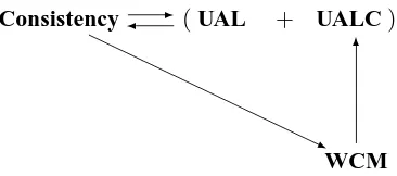
The logical relationships between the concepts of consistency, UAL, UALC and WCM are shown in graph form in Figure 1. Note that we already saw that consistency implies WCM (since consistency implies consistency in mean, which implies WCM), and that UAL combined with UALC implies consistency (shown immediately after the statement of Theorem 4). Instead of prov-ing directly that consistency implies UAL and UALC, we will prove that WCM implies UALC, and hence that consistency implies UALC. Consistency combined with UALC, in turn, implies UAL, since
Dn
f,f¯|{Q(Rk)}
{Rk}
≤Dn(f,f∗) +Dn
¯
f|{Q(Rk)}
{Rk} ,f
∗→0
Consistency- (UAL + UALC)
WCM
6
-Figure 1: Logical relations between consistency, Uniform Approximate Localizability (UAL), Uni-form Approximate Local Consistency (UALC) and Weak Consistency in Mean (WCM). That is, consistency is equivalent to the combination of UAL and UALC; consistency implies WCM; and WCM implies UALC.
Lemma 6 A learning method that is WCM is UALC.
The proof of Lemma 6 is the most complex of our results; we now sketch it very briefly (the full proof appears in Appendix B). The initial idea is to consider Sn(x,r)as|Sn(x,r)|points derived from
Px,r. The expected loss of a smoothed local version can then be seen to be approximately equal to
a mean of expected losses over Px,r for various x. The expected losses over Px,r can, in turn, be
bounded by the MADs of fP∗x,r and f as well as the difference between their means; we bound the latter two using the WCM property. Finally, we construct in a recursive manner Q and{Rk}that
fulfill the requirements of UALC, using some results from measure theory regarding the asymptotic behavior of fP∗x,r.
Based on our results thus far, as summarized in Figure 1, it is obvious that we can also conclude the following:
Corollary 7 A learning method is consistent iff it is both UAL and WCM.
This can be stated as
Consistency ⇐⇒ UAL⊕WCM
since just like UAL and UALC, UAL and WCM are clearly independent in that neither implies the other, in fact, the same two examples seen in (3) apply here: fy has already been mentioned to be
WCM, while clearly it is not UAL, whereas f0is UAL but not WCM. 6. Localizable Sets of Distributions
Thus far we have been concerned with consistency in the sense of the set of all (appropriately bounded) distributions; this is a very general case. However, many specific types of learning prob-lems consider more limited sets of distributions. Our goal in this section is to apply our results to such problems. In addition, this section will provide some of the tools used in Section 7 to derive results for classification.
This section relies on the following definition:
Definition 8 We call a set of distributionsPlocalizable iff
That is, a localizable set of distributions contains all conditionings of its distributions onto small balls. Simple inspection of the proof of Lemma 6 reveals that it holds true on localizable sets of distributions, and not just on the set of all distributions, simply because we apply the WCM property of f only on distributions Px,r. Consequently, it is easy to see that our results—specifically, Theorem
4 and Corollary 7—apply to localizable sets in general, and not just to the set of all distributions bounded by some constant M>0 (which is just one type of example of a localizable set). Note that the requirement that a set of distributions be localizable is in a sense the minimal requirement we would expect, since if f is consistent on a distribution P but not on some Px,rthen there is no reason
to expect f to be UALC. We will say more about this matter in Section 8.
Are all standard learning problems defined (perhaps implicitly) on localizable sets of distri-butions? The answer is no; for example, if we assume that Ey=0, which implies Exf∗(x) =0,
then this is clearly not necessarily preserved when we consider some Px,r. However, the converse
is true for many standard setups in statistics and machine learning. Specific examples include the following, to all of which our results apply (assuming the boundedness assumption is upheld):
1. y= f∗(x) +ε , εis independent of x , Eε=0
This is the standard regression model with additive noise (and random design) appearing in statistics. It is clearly a setup that implicitly works on a localizable set since Px,r retains the
property that y= f∗(x) +ε.
2. As a subcase of the previous example, we can assume that f∗∈
F
, whereF
is the set of all continuous functions, or alternatively some ‘smoothness class’, for example, Lipschitz-continuous functions, etc. Note, however, that if the density of the marginal distribution on X is assumed to be bounded then this is no longer a localizable set.3. P y= f∗(x)=1 , ∀S,x f(S,x),f∗(x)∈ {−1,+1}
This is a noiseless classification problem, or set-estimation problem with non-overlapping sets, since
P f(Sn,x)6=y
=ESn,(x,y)1
f(Sn,x)6=y =
1 2ESn,x
f(Sn,x)−f∗(x)
=1
2Ln(f).
That is, the 0-1 loss used in classification is equal to (half) the
L
1 loss in this case. Note,however, that we assume f(S,x)∈ {−1,+1}, and smoothed local versions do not have this property; for them the equality between the 0-1 and
L
1 losses is not valid. If we are willingto use the
L
1norm for classification, however, then our results apply here.In the next section we will see a way to derive results for the 0-1 loss, as well as allow noisy distributions, that is, the standard classification setup. This will require somewhat different definitions than those used for regression.
4. x=φ(z)for some random variable z, whereφ: Rd→RDis smooth and D>d.
We conclude with this final somewhat more complex example in order to show how local-izable sets can be present even in settings where we might not expect them. In the setting described here, the original data(z,y) lies on some low-dimensional space, but we observe
e.g., Roweis and Saul, 2000; Belkin and Niyogi, 2003); recently such methods have been applied to supervised learning (see, e.g., Kouropteva et al., 2003; Li et al., 2005). Note also the relevance to the kernel trick, in which a kernel implicitly defines such a transformationφ. The assumption of x=φ(z) (and thatφis smooth) is a nontrivial requirement; however, it is easy to see that if we consider the set of all φand z then this set is a localizable set of distributions.
7. Classification
As mentioned in the previous section, noiseless classification in the
L
1norm can be dealt with usingthe results we have seen thus far, but this is quite limiting. Therefore in this section we consider the standard case of classification, using the natural 0-1 loss, and allowing for the possibility of noise.
In classification (also known as pattern recognition; Devroye et al., 1996) we consider only distributions for whom Y={−1,+1}; when we say ‘all distributions’ in this section we mean only distributions of this sort. Note that such distributions form a localizable set, and thus we might expect our results to apply to them. Note also that f∗(x) =E(y|x) =2η(x)−1 where η(x) = P(y=1|x), the conditional probability. We call a learning method c a classifier iff∀S,x c(S,x)∈
{−1,+1}. We will use c,d, etc., to denote classifiers, to differentiate them from general learning
methods, which we generally denote f,g.
In classification the natural loss is the 0-1,
R0−1(c) =P(c(Sn,x)6=y) =ESn,(x,y)1{c(Sn,x)6=y} and the minimal (Bayesian) loss is
R∗0−1=inf
h Ex,y1{h(x)6=y}
where the infimum is taken over all measurable h. Denote the optimal (Bayesian) classification rule by
c∗(x) =sign(f∗(x)) =sign(2η(x)−1)
which clearly minimizes R0−1. We are interested in the relative loss∆R0−1(c) =R0−1(c)−R∗0−1.
This is well-known to be equal to (half the value of)
e
Ln(c)≡ESn,x|c(Sn,x)−c∗(x)| · |2η(x)−1|=ESn,x|c(Sn,x)−c∗(x)| · |f∗(x)|.
That is, we have the usual
L
1 loss but it is weighted according to the distance ofη(x)from 1/2.Another difference is that we compare c to c∗=sign(f∗)and not to f∗. These differences between
e
Ln and the loss Ln we considered in the main part of this work prevent an immediate application
of our results. We will therefore present alternative definitions that will allow us to get around this problem.
First, we define mutual consistency in the context of classification, which we will call mutual
classification-consistency (or, briefly, mutual C-consistency), using
e
Dn(c,d) =ESn,x|c(Sn,x)−d(Sn,x)| · |2η(x)−1| −→0
—that is, we simply add the same weighting as ineLn. This leads to defining classification-consistency
(or, briefly, C-consistency) on a distribution P as
e
(denoting c∗(S,x) =c∗(x)). Note that, in a similar way as in regression, C-consistency is a specific case of mutual C-consistency.
A change needs to be made to smoothed local versions to ensure that they remain classifiers, since ¯c|qrcan return values not in{−1,+1}. Define, therefore,
e
c|qr(S,x) =sign(c¯|qr(S,x)) =sign Ex′∼Px,qrc(S(x,r),x′).
When we talk of smoothed local versions in the context of classification, we intendec|qr.
We can now define a version of UAL for the context of classification, in the following natural way. Let C-UAL be the same as UAL, but replace DnwithDen, f with c and ¯f|qr withec|qr.
Instead of proving results ‘from scratch’ for the definitions given in this section, we can build upon the previous ones, using the following general technique. Let fkerbe a consistent
Nadaraya-Watson kernel estimator using the window kernel. Define
f|·|(S,x) =|fker(S,x)|.
For any classifier c, define a learning method
fc(S,x) =c(S,x)f|·|(S,x).
We can see fc(S,x)as an estimate of f∗(x), using (in a plug-in manner) c(S,x)to estimate sign(f∗(x))
and f|·|(S,x)to estimate|f∗(x)|.
We will now use our results on regression for estimators fc in order to arrive at conclusions
for classifiers c. Note that |fc(S,x)| ≤1 (since fker uses the window kernel, it is bounded by the
largest|yi|in the training set, which is 1). Given the additional fact that in classification we have
Y={−1,+1}, we can conclude that our boundedness assumption on learning methods is of no con-sequence to our treatment of classification, that is, to get completely general results for classification we need only rely on bounded regression with M=1.
To arrive at results, we will need some minor facts:
Lemma 9 The following hold true for every P,c,d:
1. Dn(fc,fd)→0 ⇐⇒ Den(c,d)→0.
2. Dn(fc,f∗)→0 ⇐⇒ Den(c,c∗)→0.
3. fcis UALC ⇒ Dn
¯
(fc)|{{QR(Rk)}
k} ,fc˜|{Q({RkRk} )}
→0
for large-enough Q,{Rk}in the sense appearing in the definitions UAL,UALC.
The first part of the lemma indicates that the C-mutual consistency of any c,d are linked to the
mutual consistency of fc,fd; the second does the same for C-consistency and consistency. The third
part of the lemma shows that if fc is UALC then smoothed local versions of fc are asymptotically
equivalent to fc′, where c′ is a smoothed local version in the sense of classification of c (in other words, we can either smooth fcor first smooth c and then apply f ; the result is similar). A proof of
all parts of the lemma appears in Appendix E.
Lemma 9, hence by Theorem 4 (and what we have seen regarding localizable sets in Section 6) fc
is UAL onP, that is, for every P∈Pwe have
Dn
fc,(f¯c)|{{RQ(Rk)}
k}
→0
for large-enough Q,Rk in the sense of the definition of UAL. fc is also UALC onP, and therefore
for large enough Q,Rkwe have
Dn
¯
(fc)|{{QRk(}Rk)},fc˜
|{Q({Rk}Rk)}
→0
by part 3 of Lemma 9, and therefore we conclude by the triangle inequality that (again, for large enough Q,Rk)
Dn
fc,fc˜
|{{Q(RkRk} )}
→0.
Hence, by part 1 of Lemma 9, c and ˜c|{Q(Rk)}
{Rk} are mutually C-consistent for large-enough Q,Rk, that is, c is C-UAL on P. Since this was for every P∈P, we conclude that c is C-UAL onP. Since the
entire argument was for an arbitrary localizable setP, we conclude that
Theorem 10 A C-consistent classifier on a localizable setPis C-UAL onP.
In particular, since the set of all distributions (having Y ={−1,+1}) is localizable, we get
Corollary 11 A C-consistent classifier is C-UAL.
In a similar way we can define in the context of classification concepts parallel to UALC and WCM, and prove corresponding results (we do not go into details to avoid repetition).
8. Concluding Remarks
Our analysis of consistency has led to the following result: Consistent learning methods must have two properties, first, that they behave locally (UAL); second, that their mean must not be far from estimating the true mean (WCM). Only a learning method having these two independent properties is consistent, and vice versa; their combination is logically equivalent to consistency.
To further elaborate on this result, note that UAL is clearly a local property, and WCM a global one. Thus, we can see consistency as comprised of two aspects, one local and one global. Note also that the global property, WCM, is a trivial consequence of consistency, and therefore what is worth noting about this result is that consistency implies local behavior. We can then ask, in an informal manner at least, why is this so?
As noted in the introduction, the loss Lnthat we considered is a global one, in that we average
to be useful on other data sets; specifically, assume that f is consistent. We can then calibrate its output so that it returns an empirical mean of 0, which makes sense since we know that Ey=0. That is, let
g(S,x) = f(S,x)− 1
|S|i=
∑
1..|S|f(S,xi)(alternatively, we might calibrate by multiplying by an appropriate scalar, etc.). Then, while g is consistent on the set of distributions with Ey=0 (using the consistency of f on all distributions),
g does not behave locally. This can be seen, for example, by considering g on a distribution with x
uniform on[−1,1]and y=sign(x). This distribution fulfills Ey=0, and g is consistent on it, but neither UAL nor UALC, since smoothed local versions of g in fact return values tending towards 0.
Thus, in summary, the fact that the set of all distributions is localizable is what causes consis-tency to imply local behavior. If we are concerned about that fact (e.g., because we suspect local behavior might lead to the curse of dimensionality; Bengio et al., 2006), then we must do away with consistency on the set of all distributions and instead talk about consistency on a more limited set, one which is not localizable. However, part of the reason why nonparametric methods often outperform parametric ones on real-world data is precisely because they make as few as possible assumptions about the unknown distribution. Consequently, we may find that local behavior is hard to avoid.
We now turn to directions for future work. One such direction is to apply our results towards proving the consistency of learning methods not yet known to be consistent. It appears that in many cases proving the WCM property should not be difficult; hence, what remains is to prove UAL. While not necessarily a simple property to show, it may in some cases be easier than proving consistency directly.
An additional area for possible future work is empirical investigation, as follows. Since a con-sistent method is necessarily UALC, we can consider using a smoothed local version of the original method, since if chosen appropriately it is also consistent.2 Now, if for example we have a large training set and only a few points at which to estimate, then by training on the local parts of the original training set we may save time. Of course, there is no guarantee that this will be beneficial on a particular problem, since consistency is an asymptotic property. Future empirical work might therefore examine real-world data sets in detail to see how the performance of local versions of a method compare to the original.
Acknowledgments
We thank the anonymous reviewers of a previous version of this paper for their comments. We also acknowledge support for this project from the Israel Science Foundation as well as partial support from NSF grant DMS-0605236.
2. Note that we might not need smoothing in practice, since the smoothing radius becomes negligibly small, Q(Rk)Rk=
Appendix A. Proof of Proposition 1
For any sample S, denote the mean and standard deviation (of the xs) by
ˆ
E(S) = 1
|S|i=
∑
1.. |S|xi , σˆ(S) =
s
1
|S|i=
∑
1.. |S|xi−Eˆ(S)
2
.
Now, start with a consistent method g, which is translation-invariant in the sense that
∀S,x,b g(S,x) =g(S+b,x+b)
where S+b={(xi+b,yi) : (xi,yi)∈S}(for example, we can take g to be a kernel estimator).
Define, for any q>0,
fq(S,x) =
(
g(S,x) x∈/BEˆ(S),qor x∈ {xi : (xi,yi)∈S}
0 otherwise
and let
Q(S) = σˆ(S)
log(|S|).
Finally, let
f(S,x) = fQ(S)(S,x).
We will first show that f is consistent; then we will show that f is neither locally consistent nor localizable. A brief overview of the proof is as follows: As n→∞, we get that Q(Sn)≈logconst(n). This
means that f is forced to return 0 on an area with vanishing radius, and hence f behaves like g on an area with measure rising to 1, and is consistent. On the other hand, when we consider a local version, we get that Q(Sn(x,Rn))≈O
Rn
log(m)
, where m is the size of Sn(x,Rn). We also get that x,
the point at which we are estimating, is at distance≈O
Rn
√m
from ˆE(Sn(x,Rn)), a distance which
is asymptotically smaller than Q. Hence x will tend to be in the area on which f is forced to return 0, making f neither locally consistent nor localizable.
We now start with the formal proof, first showing that f is consistent. Since X is bounded, ˆ
σ(Sn) is bounded, and hence Q(Sn) =logσˆ(S(nn)) →0. We first assume that there is not a point mass
on Ex, which implies µ
BEˆ(Sn),Q(Sn)
→0 almost surely, which follows from the fact that, since ˆ
E(Sn)→Ex a.s. (by the LLN) and Q(Sn)→0, we must have lim supnBEˆ(Sn),Q(Sn)⊆ {Ex} with
probability 1. We can then use the consistency of g to see that
ESnEx|f(Sn,x)−f∗(x)|
≤ESnEx1{x∈/BEˆ(Sn),Q(Sn)or x∈ {xi : (xi,yi)∈Sn}}|g(Sn,x)−f
∗(x)|
+ESn2Mµ
BEˆ(Sn),Q(Sn) \
{xi : (xi,yi)∈Sn}C
≤ESn
h
Ex|g(Sn,x)−f∗(x)|+2Mµ
BEˆ(Sn),Q(Sn)
i
which proves that f is consistent. Consider now the case where there is a point mass on Ex. Recall that lim supnBEˆ(Sn),Q(Sn)⊆ {Ex}a.s., and note that due to the point mass on Ex, we have P Ex∈ {xi : (xi,yi)∈Sn}
→1. Because of these two facts, we get
ESnµ
BEˆ(Sn),Q(Sn) \
{xi : (xi,yi)∈Sn}C
→0
hence once more f is consistent by the consistency of g, by a similar argument as before.
We will now show that f is not locally consistent. For this, it is sufficient to show a single distribution on which Ln f|{Rk}
does not converge to 0, for any sequence Rk→0. Take X= [0,1]
(higher-dimensional cases can be proved similarly), let µ be uniform on X , and let y= +1 with probability(1+f∗(x))/2, and otherwise y=−1 (which makes sense if f∗(x)∈[−1,+1]). Define
f∗(x) =
(
+1/2 x∈0,1 2
−1/2 x∈ 12,1.
Fix some x∈(0,1). Note that µ has no point masses, so P(x∈ {xi : (xi,yi)∈Sn}) =0, and the
relevant condition in the definition of fq is of no consequence. Now, for large enough n (that is,
small enough Rn) we have x∈[Rn,1−Rn]; we will now focus on that case.
Denote Se=Sn(x,Rn) and m=m(n,x,Rn) =|Se|. Notice that m is the sum of i.i.d Bernoulli
variables, and that
Em=2nRn , σ2(m)≤2nRn (6)
(recall that Em,σ2(m) denote the expected value and variance of the random variable m,
respec-tively). Now, consider the case in which nRn 6→∞. Then there is some bounded subsequence,
knRkn ≤K for all n. Then (using Chebyshev) clearly m is less than 4knRkn with non-vanishing prob-ability on this subsequence. Since Rk →0 then in order for f to be consistent we must, for large
enough n, discriminate between the two possibilities f∗(x) = +1/2,f∗(x) =−1/2 in a way that does not depend upon x (due to the invariance of f , which stems from the translation-invariance of g). But discriminating between the two cases with arbitrarily small error cannot be done with a bounded sample size, hence the loss cannot go to 0. Thus, we conclude that if nRn6→∞
then f is not locally consistent.
Consider now the other case, of nRn→∞. We start by formulating bounds for m,|x−Eˆ(Se)|,
and ˆσ2(Se).
• m: Using Bernstein’s Inequality and (6), we get
P(|m−2nRn| ≥t)≤2 exp
−12 t 2
2nRn+t/3
.
Picking t=tn=nRn, we get
P(|m−2nRn| ≥nRn)≤2 exp
−16nRn
. (7)