REAL-TIME OPERATING SYSTEMS AND WIRELESS NETWORKS
by
Andrew Jacob Wolin
A thesis
submitted in partial fulfillment of the requirements for the degree of Master of Science in Computer Engineering
Boise State University
DEFENSE COMMITTEE AND FINAL READING APPROVALS
of the thesis submitted by
Andrew Jacob Wolin
Thesis Title: On Designing Collaborative Robotic Systems with Real-Time Operating Systems and Wireless Networks
Date of Final Oral Examination: 21 November 2014
The following individuals read and discussed the thesis submitted by student Andrew Jacob Wolin, and they evaluated his presentation and response to questions during the final oral examination. They found that the student passed the final oral examination.
Sin Ming Loo, Ph.D. Chair, Supervisory Committee John N. Chiasson, Ph.D. Member, Supervisory Committee
Hao Chen, Ph.D. Member, Supervisory Committee
iv
I would like to thank my Lord and Savior Jesus Christ. Apart from Him I can do nothing. “Delight yourself in the Lord, and He will give you the desires of your heart.” Psalm 37:4
I would like to thank my thesis advisor, Dr. Sin Ming Loo, for allowing me to pursue this work. His knowledge and experience was an invaluable guide during the research. I would like to thank committee members Dr. John Chiasson and Dr. Hao Chen for their support, time, and guidance. They are true engineers, mathematicians, and mentors. I would like to thank the highly talented members of the Hartman Systems Integration Lab for sharing their experience and insight into the world of embedded systems.
I would like to thank my father, Dale, who is an engineer by birth and has always inspired new and interesting innovations. Thanks to my mother, Lois, who has always gone to great lengths to take care of me. Thanks to my brother, Jason, a computer natural who started programming an HP 48S in his early youth. Thanks to my brother, Joe, who has been an inventor and entrepreneur even before graduating high school. Thanks to Jon and Carol for their love and support.
v
Robotic devices currently solve many real-world problems but do so primarily on an individual basis. The ability to deploy large quantities of robots to solve problems has not yet been widely embraced partially due to the complex nature of robotics and levels of research investment.
Existing research in robot collaboration largely exists in the forms of models and simulations. This work seeks to accelerate the next level of research in this area by providing a low cost, collaborative capable robotic system. This platform can be used as a gateway to transport simulations into physical representations. This research not only presents a completed robot but also provides a guide for fellow researchers to use when custom tailored systems are required.
vi
ACKNOWLEDGEMENTS ... iv
ABSTRACT ... v
LIST OF TABLES ... xi
LIST OF FIGURES ... xii
LIST OF ABBREVIATIONS ... xv
CHAPTER 1: INTRODUCTION ... 1
1.1 Solving Problems with Robots ... 1
1.2 Solving Problems with Many Robots ... 2
1.3 Swarm Robotics vs Collaborative Robotics ... 2
1.4 Summary of Definitions for this Research... 4
1.5 Thesis Framework ... 5
CHAPTER 2: PREVIOUS WORK AND EXISTING TECHNOLOGY ... 6
2.1 Group Robotics ... 6
2.2 Collaboration Using ZigBee Protocol ... 8
2.3 Existing Robotic Platforms ... 10
2.4 Summary ... 11
CHAPTER 3: THE DESIGN PROCESS ... 12
3.1 Task Dependency and Workflow... 12
vii
4.1 Integrated Motor Features ... 15
4.1.1 Encoders ... 16
4.1.2 Gear Reduction ... 16
4.2 Motors ... 16
4.2.1 Brushed DC ... 17
4.2.2 Stepper Motor ... 17
4.2.3 Servo Motor... 18
4.2.4 Continuous Rotation Servo Motor ... 19
4.3 Surplus Motors ... 20
4.3.1 Faulhaber 1524E006S123 ... 20
4.3.2 Motor Summary ... 20
4.4 Wheel and Hub ... 21
4.5 Microcontroller ... 23
4.6 Power Supply ... 24
4.7 Summary ... 28
CHAPTER 5: MECHANICAL DESIGN ... 29
5.1 Required Skillset ... 29
5.2 3D Printing Technologies ... 30
5.2.1 Form1 - Stereolithography (SLA) ... 31
5.2.2 Maker Bot 2 - Fused Deposition Modeling (FDM) ... 31
5.2.3 Shapeways - Selective Laser Sintering (SLS) ... 31
viii
5.3.2 Chassis Revision 2 - Material Reduction ... 33
5.3.3 Chassis Revision 3 - Motor Rotation ... 34
5.3.4 Chassis Revision 4 - Increase Stability ... 36
5.3.5 Summary of Build Material and Cost ... 37
5.4 Evaluation of Technologies ... 37
5.5 Summary ... 38
CHAPTER 6: HARDWARE DESIGN AND CONFIGURATION ... 39
6.1 Microcontroller Configuration ... 40
6.1.1 Boot Modes ... 40
6.1.2 Clock Source ... 41
6.1.3 Crystal Selection and Configuration ... 43
6.1.4 Clock Speed Configuration ... 48
6.2 Programming/Debugging ... 50
6.2.1 Serial Wire Debug ... 50
6.2.2 USART/UART/RS232 ... 52
6.2.3 Combining SWD and USART into One Cable ... 53
6.3 Power System... 55
6.4 Motor Control ... 56
6.4.1 H-Bridge Circuit ... 56
6.4.2 Speed Control ... 57
6.4.3 Stopping vs Braking ... 58
ix
6.5.2 SFH 7773 Integrated IR Emitter and Detector ... 61
6.6 Communication ... 68
6.7 Assembled Motherboard PCB ... 69
6.8 Summary ... 71
CHAPTER 7: FINAL ASSEMBLY ... 73
7.1 Summary ... 75
CHAPTER 8: SOFTWARE DESIGN ... 77
8.1 Cooperative Scheduling ... 77
8.2 Preemptive Scheduling ... 78
8.3 Real-Time Operating System ... 78
8.4 Software Layers ... 79
8.5 Threading Model ... 80
8.6 Collaboration in Hardware and Software ... 81
8.6.1 Identical Code Base ... 81
8.6.2 Unique Identification... 81
8.6.3 Robot States... 82
8.6.4 Atomic Access to Hardware ... 83
8.7 Collaboration Algorithms ... 83
8.8 Summary ... 87
CHAPTER 9: TEST RESULTS AND HARDWARE VERIFICATION ... 88
9.1 Battery Pack Discharge Data ... 88
x
9.2.2 LTE-302/LTR-301 Distance Measurements - With Shroud ... 91
9.2.3 LTE-302/LTR-301 Shroud vs No Shroud Comparison ... 92
9.2.4 LTE-302/LTR-301 Noise Test ... 93
9.2.5 LTE-302/LTR-301 Response Time ... 94
9.3 FSH 7773 Proximity Sensor Test Results ... 95
9.3.1 Distance Measurement Data... 95
9.3.2 FSH 7773 Ground Isolation ... 97
9.4 Proportional Derivative Controller ... 100
9.5 Testing Collaboration... 103
9.6 Summary ... 105
CHAPTER 10: CONCLUSIONS AND FUTURE WORK ... 106
10.1 Mechanical Changes ... 106
10.2 Sensor Changes ... 107
10.3 Robot vs Wall Detection ... 108
xi
Table 1.1 Group Robotics Naming Conventions ... 4
Table 4.1 Motor Relative Generalizations ... 16
Table 4.2 Motor Summary ... 21
Table 4.3 Battery Relative Generalizations ... 25
Table 4.4 LiPo/LiFePO4 Pack Cost Comparison ... 27
Table 4.5 LiPo / LiFePO4 Electrical Characteristics ... 27
Table 5.1 Material and Cost by Revision ... 37
Table 6.1 STM32F4 Boot Modes ... 41
Table 6.2 STM32F4 Memory Map of Bootable Regions ... 41
Table 6.3 Clock Options and Associated Speeds ... 42
Table 6.4 8 MHz crystal datasheet values ... 44
Table 6.5 Solutions to Equation 6.7 ... 46
Table 6.6 PLL Scale Factor Descriptions and Values ... 49
Table 6.7 RJ45 to SWD/RS232 Pinout ... 54
Table 6.8 Estimated Component Max Power Breakdown ... 55
xii
Figure 2.1 Mesh Network ... 9
Figure 2.2 Star Network ... 10
Figure 3.1 Design Workflow ... 13
Figure 4.1 Brushed DC Motor ... 17
Figure 4.2 Stepper Motor ... 18
Figure 4.3 Servo Motor Breakdown ... 18
Figure 4.4 Continuous Rotation Servo ... 19
Figure 4.5 Motor Mounts and Hubs ... 22
Figure 4.6 Motor, Hub, and Wheel Disassembly ... 23
Figure 5.1 Mechanical Prototype - Revision 1 ... 33
Figure 5.2 Mechanical Prototype - Revision 2 ... 34
Figure 5.3 Mechanical Prototype - Revision 3 ... 36
Figure 5.4 Mechanical Prototype - Revision 4 ... 36
Figure 6.1 Hardware Block Diagram ... 39
Figure 6.2 Recommended layout for an oscillator circuit ... 47
Figure 6.3 SWDCLK signals - 16” jumper wires ... 52
Figure 6.4 RJ45 Ethernet Connector ... 53
Figure 6.5 RJ45 Programming / Debug Setup ... 54
xiii
Figure 6.8 SFH 7773 Datasheet Schematic ... 64
Figure 6.9 MCP1702 - Dynamic Load Response... 64
Figure 6.10 Ground Isolation for SFH 7773 Power Supply ... 66
Figure 6.11 FSH 7773 Daughter Card... 67
Figure 6.12 FSH7773 Proximity Sensor Daughter Cards ... 67
Figure 6.13 XBee Schematic and Debug LEDs ... 69
Figure 6.14 Robot Motherboard - Front ... 70
Figure 6.15 Robot Motherboard - Back ... 71
Figure 7.1 Robot Disassembled... 73
Figure 7.2 Assembled Robot - Front ... 74
Figure 7.3 Assembled Robot - Back ... 74
Figure 7.4 Assembled Robot - Bottom ... 75
Figure 7.5 Robot with Programmer/Serial Port... 75
Figure 8.1 Software Layers ... 80
Figure 8.2 Threading Model ... 81
Figure 8.3 Group Obstacle Avoidance ... 84
Figure 8.4 Outward Dispersion Algorithm... 85
Figure 8.5 Linear Dispersion Algorithm ... 86
Figure 8.6 Top Level Collaboration Algorithm ... 86
Figure 9.1 LiFePO4 vs LiPo - Discharge Data ... 89
Figure 9.2 No Shroud - 1 IR LED on ... 90
xiv
Figure 9.5 Shroud - 1 IR LED on ... 91
Figure 9.6 Shroud - 3 IR LEDs on ... 92
Figure 9.7 Shroud - 1 vs 3 IR LEDs on ... 92
Figure 9.8 Shroud vs No Shroud - 3 LEDs on ... 93
Figure 9.9 No Shroud, 3 LEDs On, 5cm - 1 second noise test... 94
Figure 9.10 IR Phototransistor Response Time... 95
Figure 9.11 FSH 7773 Left... 95
Figure 9.12 FSH 7773 Right ... 96
Figure 9.13 FSH Left vs Right ... 96
Figure 9.14 FSH 7773, 5cm - 1 second noise test ... 97
Figure 9.15 FSH 7773 - VDD using a common ground ... 98
Figure 9.16 FSH 7773 - V_LED using a common ground ... 98
Figure 9.17 FSH 7773 - VDD using ground isolation ... 99
Figure 9.18 FSH 7773 - V_LED using ground isolation ... 100
Figure 9.19 PD Error - Proportional Component ... 101
Figure 9.20 PD Error - Derivative Component ... 102
Figure 9.21 PD Error - Total ... 102
Figure 9.22 Multiple Robots ... 103
xv ADC Analog-to-Digital Converter
cm Centimeter
DC Direct Current
GPIO General Purpose Input/Output
IR Infrared
I/O Input/Output
I2C Inter-Integrated Circuit
IGRS Intelligent Grouping and Resource Sharing ISR Interrupt Service Routine
LED Light Emitting Diode
mm Millimeter
mV Millivolt
PWM Pulse Width Modulation PCB Printed Circuit Board
RF Radio Frequency
RTOS Real-Time Operating System SPI Serial Peripheral Interface TI Texas Instruments
USB Universal Serial Bus
CHAPTER 1: INTRODUCTION
1.1 Solving Problems with Robots
One of the most amazing displays of early robotics was the invention of a remote controlled submergible boat. In 1898, Tesla demonstrated a contraption that was far ahead of its time. It was able to receive radio signals, and therefore commands, to move forward, turn, submerge, and toggle lights [1]. It was perhaps so far ahead of its time that the idea of robotic minions was not ready to be accepted by the public or even the
military. Attempts at purely mechanical and analog robots were made during the early 1900s. The real fuel to the robotic revolution came with the invention of the solid state transistor in 1947. As advancements in computing were made, robotic creations followed. As programs were written to solve basic math problems the possibilities became readily apparent for computers to join themselves to other electric and mechanical machines.
One of the first robotic inventions ever produced, sold, and made to perform useful work arrived in 1961. The robot was named Unimate and was used in a General Motors assembly line to perform work that was difficult for humans to do. With significant changes in the world since Tesla’s idea, society was ready to accept the idea of robots assisting mankind [2].
Federation of Robotics reports that Japan was the largest producer of robots in the world [3]. Japan has also taken an interest in humanoid robotics and has led several innovations in that field. As an example, Japanese manufacturer Honda has produced the famous humanoid robot ASIMO, an acronym for Advanced Step in Innovative MObility. ASIMO is able to interact with people by recognizing human gestures, sounds, and shapes.
1.2 Solving Problems with Many Robots
Solving a simple problem with a single robot, autonomous or semi-autonomous, is by itself a challenging task. The rewards for meeting the challenge are huge and have led to the betterment and saving of human lives through advanced prosthetics, wheel chairs, and implants. From the depths of the ocean to distant mars, robots have served as competent explorers into the unknown. Taking this technology and enabling it to work as a group, collectively, is the idea behind collaborative problem solving with robotics [4].
1.3 Swarm Robotics vs Collaborative Robotics
Swarm robotics is a specific type of group robotics that has emerged over the last ten years. It has produced very interesting collective behaviors inspired by insect groups. The exact definition of swarm robotics is somewhat undefined. In general, the common goal is to have the robotic group interact with each other, but not communicate with each other using a single intelligent organizer like a computer [5]. Applying this limitation on the discipline of swarm robotics forces the research to solve problems in a highly
redundant and scalable manner. The robots interact with each through similar
robotics has been compiled at the Universite Libre de Bruxelles. The following series of steps will demonstrate a simple algorithm to explain swarm robotics [6].
1) All robots are tasked to find a light hanging from the ceiling. 2) Initially all robots emit red light around their body.
3) If a robot detects another red robot, it changes direction and continues searching. 4) If a robot detects the light, it changes color to blue.
5) If a robot detects the now blue robot, it latches on and changes color to blue. 6) Once all robots detect the light, all are blue and latched together.
In this example, a problem has not necessarily been solved but the robots have self-organized based on a simple set of rules. All of these activities are done using passive forms of communication as the robots merely sense changes to neighboring robots color. It is a completely different way to solve problems and has led to exciting new possibilities.
and concentrated. Since the members must travel potentially large distances from each other, they cannot use the swarm mechanisms used by swarm robotics to interact. They must communicate in an active way with each other to coordinate the large-scale work and relay critical information such as discovery of the lost or wounded.
Many of the ambitions of swarm robotics agree with collaborative robotics in that many robots, costing as little as possible, should be used to solve a problem. Unlike swarm robotics, however, it is important to this innovation that there are few restrictions. If the most effective solution is to have multiple groups of different types of robots combine to solve the problem, then this is the superior solution until a new solution is discovered.
1.4 Summary of Definitions for this Research
The terminology in this study conforms to existing terminology as best as
possible. The terms, “group,” “swarm,” “collaborative,” and “cooperative” are so similar in lexical meaning that some well-placed definitions will aid in understanding the
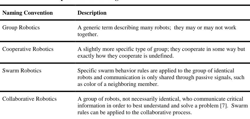
differences. Table 1.1 describes the differences in order from generic to more specific. Table 1.1 Group Robotics Naming Conventions
Naming Convention Description
Group Robotics A generic term describing many robots; they may or may not work together.
Cooperative Robotics A slightly more specific type of group; they cooperate in some way but exactly how they cooperate is undefined.
Swarm Robotics Specific swarm behavior rules are applied to the group of identical robots and communication is only shared through passive signals, such as color of a neighboring member.
1.5 Thesis Framework
CHAPTER 2: PREVIOUS WORK AND EXISTING TECHNOLOGY
This chapter focuses on existing technology in the field of design and fabrication of collaborative robotics.
2.1 Group Robotics
Many forms of group robotics exist. Their application stretches from the bottom of the ocean to the depths of space. Researchers at California’s Institute of Technology Jet Propulsion Laboratory have begun work that will aid the construction of buildings on Earth’s moon and even Mars [8]. Construction work such as this requires a collaborative effort at times. Multiple types of robots are likely to be deployed and the technology must exist where a robot can call upon another robot that has the specialized tool set to solve the problem. Their work uses an outdoor-like laboratory setting to perform the experiments. The robots are much larger than the platform proposed in this research and consequently expensive. The low robot counts result in fewer collaborative tests. It would be beneficial for the research to use scaled down versions of the hardware for experimentations on a lab table. Once collaboration experiments have been performed on the scaled model, the results can then be applied and further testing can continue on the large-scale robots.
semi-autonomous. Research performed by Tauchi et al. [9] has demonstrated interesting simulations where robots are assigned one of three different types of personalities and then deployed into a fully autonomous mode. In order to collaborate most effectively, the robots discover one another’s personalities and then solve a problem by grouping
according to the same personality. These simulations show the need for efficient
collaboration and have set the stage for additional research. The next logical step for this research is to port the simulation to actual hardware that can support multiple threads and task management.
Similar to the research described in [9], Wang et al. [10] have developed a model where each robotic node has a concept of intention much like a human has intention to solve problems. When multiple robots all share a common intention, resolution must be made on how the robots will work together in order to solve the problem. This involves fairly complex algorithms in order to overcome the inherent contention in collaborative robotics. It uses negotiation prediction and an equilibrium matrix in order to keep appropriate distance between the nodes. This research likely has interesting results but only exists as a model and requires a physical platform to execute.
The Massachusetts Institute of Technology Computer Science and Artificial Intelligence Laboratory (MIT CSAIL) has led several efforts toward collaborative
worker immobile. A mathematical model surrounding this type of randomness is called the Markov Decision Process (MDP). Dibangoye et al. [11] have utilized this model in collaborative robotics. Functional tasks have been demonstrated such as the ability to recognize objects too large for a single robot to move and asking for assistance from other available worker nodes.
2.2 Collaboration Using ZigBee Protocol
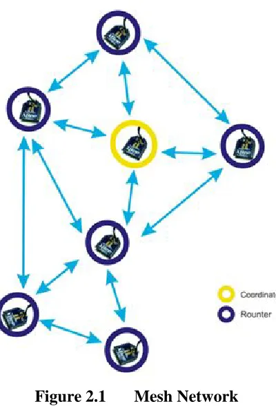
ZigBee is a RF communication protocol that adds mesh networking to the 802.15.4 radio protocol. The technology has grown rapidly since its conception and has been adapted to robotic collaboration in many unique ways. One approach to group robotics has adopted the Intelligent Grouping and Resource Sharing (IGRS) protocol as a foundation for its collaboration mechanism. IGRS was initially designed to support the resource sharing of PCs, TVs, Set Top Boxes, and mobile devices. As robotics begin to act more and more like an appliance in the home and office, this protocol should likewise be inherited by robotics. Zhiguo, Junming, Xu, Zhilang, and Jun have begun research in this area and propose the use of ZigBee wireless communication between robotic nodes which then integrate into an 802.11b/g/n home wireless network [12]. Their study is largely focused on how to provide a scalable grouping strategy based on IGRS and consequently lacks stable robotic test platforms to carry out the experiments.
Swarm robotics has taken an interest in ZigBee technology as well. The data that is communicated in swarm robotics attempts to simulate the same types of data
commission in a colony, another ant is readily available to take its place. In the same way, ZigBee is able to re-route data in the event that a node is removed from the mesh network. The network in Figure 2.1 represents the concept behind the mesh
implementation. Note that, while a client (aka router) is able to fail, the coordinator must remain active.
Figure 2.1 Mesh Network
network. This allows the use of real-time data manipulations on the higher powered PC that connects to the coordinator. An illustration of a mesh network is seen in Figure 2.2.
Figure 2.2 Star Network
Many chipsets are available that implement the ZigBee protocol. The research in [14] has selected the MG2455 manufactured by Radio Pulse. Much like the well-known XBee module, the MG2455 is able to carry out mesh and star networking between embedded systems. Two robots carried out experiments to demonstrate the usefulness of ZigBee during collaboration.
2.3 Existing Robotic Platforms
source solutions. The robot uses a hexapod leg system to move itself, which lends itself to certain environments but as a consequence it is very slow to move about. This platform is not designed for collaboration but does have desirable features such as a layered software approach that depends on an RTOS.
2.4 Summary
CHAPTER 3: THE DESIGN PROCESS
The design process involves a series of logical tasks. Some tasks can be done in parallel. Others can only be completed sequentially. This chapter discusses the
workflow in general and describes the advantages of using teams to develop products that involve many different disciplines. This design process will be referred to through the rest of the chapters.
3.1 Task Dependency and Workflow
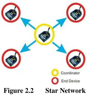
Before engaging in the development of a robotic system, a certain amount of research should be performed. Figure 3.1 shows research as the top most phase in the process. Both mechanical and hardware research should be done and existing
can be tested on small parts before fabricating large models, which will have a higher cost to produce.
Figure 3.1 Design Workflow
At this point, the software design can commit to design decisions that allow further testing of the system. Several software components will have already been
written that tested the components during the initial selection process. These components now need to be integrated into an application programming interface (API). Decisions regarding the threading model and library layers should be made before actual code production. The software design and testing phases will be repeated until all of the hardware components have been verified. Once the robot is built and tested, the targeted robotic research area of interest can begin.
The workflow allows for some phases to be done in parallel while other phases cannot move forward until the previous phase completes. The mechanical and hardware design can be done in parallel after some or all of the components have been decided on. If for example a motor has been decided upon, modeling can begin to mount the motor while bread-board testing can be done to verify circuit and software designs. This assumes that multiple researchers are available. The process is much more linear if a single researcher is tasked with the entire design.
3.2 Summary
CHAPTER 4: COMPONENT SELECTION
Robotic platforms typically integrate existing components from a variety of manufacturers. Items such as motors and batteries for example are much too costly to have custom fabricated for academic research purposes. For the initial phases of
collaborative robotic research, common low cost components are targeted since they are able to achieve sufficient accuracy for useful testing. The mechanical, hardware, and software design rely heavily on the physical dimensions and properties of these
components. The required characteristics and capabilities of the robots will help narrow the search criteria during component selection. A certain level of commitment must be made to these components before moving forward with the rest of the design. The physical components for a wheeled platform are the motor, power supply, and wheel/hub assembly. Considerations for each of these components are presented in the following sections.
4.1 Integrated Motor Features
4.1.1 Encoders
Both stepper and DC motors optionally have integrated encoders that can
determine the position of the motor shaft and send a pulse to the microcontroller for use in a control loop [16]. When a stepper motor is given the command to move 10 steps, there is only reasonable confidence that it actually moved 10 steps. An encoder built into the motor will provide feedback to the microcontroller. It reports how many steps it actually moved so that a measure of error can be taken and corrected. In a similar way, power is applied to a DC motor and the encoder counts are fed into the MCU.
4.1.2 Gear Reduction
A DC motor by itself is of limited use without the aid of gear reduction in order to achieve the necessary torque to move a meaningful amount of weight. In contrast, a stepper motor has enough torque to direct drive a small robot. A DC motor with a gear head will usually have much more torque than a stepper motor without a gearhead. For this reason, DC motors in robotics often use a gear reduction system, which could be a gearhead or pulley system.
4.2 Motors
Stepper motors and brushed DC motors are common and available platforms that can be used in small robotic applications. Table 4.1 makes relative generalizations to some of the key features of motors.
Table 4.1 Motor Relative Generalizations
Permanent Magnet AC Induction Stepper Brushless
Voltage DC AC DC AC
Top Speed Medium High Slow Very High
Cost Low Medium Medium High
4.2.1 Brushed DC
The brushed DC motor has existed much longer than a stepper motor and was used as inspiration to invent the stepper motor. The armature rotates continuously as it receives a constant or varying voltage. Control mechanisms are as simple as varying the voltage to the motor. Due to the widespread use of DC motors, all shapes and sizes can be found at reasonable prices. A DC motor is shown in Figure 4.1.
Figure 4.1 Brushed DC Motor
4.2.2 Stepper Motor
since the signaling must be absolutely precise in order for the motor to perform. Resonance and noise can interfere with the control signals causing additional design challenges. A stepper motor is shown in Figure 4.2.
Figure 4.2 Stepper Motor
4.2.3 Servo Motor
A servo motor is an embedded system that combines a DC motor, gear system, an encoder or potentiometer for feedback, and a motor controller. These components are packaged into a housing that provides a connector for the electrical connections and an output shaft to drive movement.
There are a variety of different types of servo motors but common to most of them is the control system. A 1-2 ms signal is sent to the servo, which determines which way the servo should rotate. 1 ms will rotate the servo left 90°, 1.5 ms will hold the servo at its center, and 2 ms will rotate the servo right 90°. The frequency of the signals is between 50 and 400 Hz depending on the type of servo. This is the refresh rate of the servo and consequently a higher signal frequency will provide more precise holding of the output shaft.
The simplest servo motor uses a potentiometer to provide feedback to the control circuit in order to determine absolute position. These types of servos only allow for 180° of total rotation.
4.2.4 Continuous Rotation Servo Motor
There are continuous rotation servos available that are very inexpensive ($12-$20) but they completely lack a feedback mechanism and therefore lose the ability to send absolute positioning commands. Trossen Robotics offers highly advanced servo systems that offer continuous rotation with absolute positioning and configurable parameters for the control algorithm. This is an excellent platform for demonstrations of control theory and robotics but the high feature set increases the cost. A low end robotic servo shown in Figure 4.4 starts at $140.
4.3 Surplus Motors
4.3.1 Faulhaber 1524E006S123
The simplicity of a DC motor with an encoder and gearhead is an attractive option but the cost for such a motor can be a few hundred dollars if purchased new. An
interesting surplus option was found for $23 that provides both the encoder and the gearhead. The Faulhaber 1524E006S123 can be found from surplus dealers. In addition to the gearhead and encoder, the motor comes with a 90° output shaft. Since the encoder and gearhead add considerable length to the motor, the 90° output shaft allows a pair of these motors to oppose each other vertically in a chassis, allowing for a narrow
wheelbase. Given the low price point, encoder, gearhead, and 90° output shaft, the Faulhaber was chosen as the power train, which can be seen in Figure 4.6.
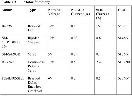
4.3.2 Motor Summary
Table 4.2 Motor Summary
Motor Type Nominal
Voltage No Load Current (A) Stall Current (A) Cost
RS395 Brushed
DC
12V 0.5 15 $5.25
SM- 42BYG011-25-
Bipolar Stepper
12V 0.33 0.6 $14.95
SM-S4203R Servo 5V 0.25 0.7 $13.95
RX-24F Continuous
Rotation Servo
12V 0.5 2.4 $139.90
1524E006S123 Brushed DC w/ Encoder, Gearhead
6V 0.2 0.5 $23.95*
* Surplus
4.4 Wheel and Hub
Figure 4.5 Motor Mounts and Hubs
The output shaft of the Faulhaber measures 7 mm in length, 3 mm in diameter, and has a flat surface for the set screw. Banebots offers a hub and wheel of appropriate size that can mount to this motor. While the hub actually measures 10 mm (3 mm
Figure 4.6 Motor, Hub, and Wheel Disassembly
4.5 Microcontroller
The embedded system requires a Microcontroller (MCU) to control the peripheral components. The end goal requirements for the robot will help determine what features are needed from the MCU. The number of peripherals, size of programmable memory, and processor speed should support the design goals. When choosing up front to use a real-time operating system, more programming space and speed should be considered. Efficiency, battery life, and cost are important selection criteria during the design but the goal is not to produce the cheapest, smallest, and most efficient design. The goal is to provide a highly robust, capable, feature-rich platform that can be used as a generic platform for individual and collaborative robotics. The power consumption of the robot can later be scaled back if needed by changing the clock speed, disabling unused features, and optimizing the code base.
Many different MCUs are available from manufacturers such as Microchip, Atmel, Texas Instruments, and STMicroelectronics. STMicroelectronics has an
This makes them an ideal supplier during research given the absence of licensing costs. The STM32F4 is a series of microcontrollers produced by STMicroelectronics. The particular model chosen from this family is the STM32F4VGT6, which is a 100-pin version containing 100 MB of user programmable flash, 82 lines of IO, and multiple ADC, I2C, SPI, UART, and USART modules. The device is capable of running up to 168 MHz, depending on the input clock configuration [18]. Many other features and abilities are available but are not used for this project. Prototyping with this particular processor is made convenient with an available demonstration board that provides access to all of the pins and has an integrated programmer.
4.6 Power Supply
Table 4.3 Battery Relative Generalizations Sealed Lead Acid (Pb) Nickel Cadmium (NiCd0 Nickel Metal Hydride (NiMh) Lithium Polymer (LiPo) Lithium Iron Phosphate (LiFePO4)
Cell Voltage 2V 1.2V 1.2V 3.7V 3.3V
Self Discharge Rate/Month
5% 20% 30% 3% 3%
Size Large Medium Medium Small Small
Charge Times
Long Medium Short Medium Very Short
Cost Low Medium Medium Medium Medium-Low
Weight High Medium High Low Medium
Energy Density
Low Medium Medium High High
Before selecting a battery, an estimation needs to be made concerning the target power requirements. Table 6.8 calculates the burst current consumption to be 3.7A and typical consumption to be approximately 1A. Lithium technology batteries have a rating that is used to calculate the rated discharge current. This is known as the “c” rating. Multiply the “c” rating by the amp hour capacity to find the discharge capabilities. Any of the above listed battery technologies could have configurations to support these voltage and current demands. The robot application will help determine what battery technology is most appropriate. For a small form factor robot such as that in this work, size, availability, and cost are the targeted features. LiPo and LiFePO4 batteries will be examined further given their small size and low cost.
The motors in this work have a nominal voltage of 6V, followed by the infrared (IR) modules using 5V, and finally the microcontroller and other ICs use 3.3V.
500mV or less. This suggests that when the pack is fully depleted, the voltage should be 6.5V or greater since a 6V regulator will be used for the motors. A 7.4V 2S LiPo pack has a charged voltage of 8.4V and a fully discharged voltage of 5.5V although 6V is typically used as a precautionary measure since over discharging a pack can damage it. This pack will work but the full energy of the pack will not be utilized since the LDO needs to regulate 6V and the dropout overhead is 500mV. In order to maximize runtime, but reduce maximum speed, the motor supply can be reduced to 5V. This would allow for the pack to drop to 5.5V even though the voltage would be cutoff at 6V for a margin of safety. Regulating the motors to 5V is a reasonable option since maximum speed is the least of concerns during a large part of the development process.
is the ability to charge 4 times faster than a LiPo. LiFePO4 also benefit in lower cost up to 50% compared to LiPo as seen in Table 4.4.
Table 4.4 LiPo/LiFePO4 Pack Cost Comparison
Manufacturer Cell Count Amp Hours (mAh) Cost
LiPo Turnigy 2 500 $4.39
LiFePO4 Zippy 2 700 $2.89
One major disadvantage of LiFePO4 over LiPo is their weight. A comparable LiFePO4 can weigh 30-40% more than a LiPo. For a small robotics application, this difference of 12 grams is of little concern. For a small, quadcopter, however this would be a significant consideration. LiFePO4 will likely continue to gain in popularity given the larger abundance of materials needed to make the battery and the greener impact on the environment but they will not entirely replace LiPo given the greater weight and lower discharge capabilities. The discharge curves of both packs will be evaluated during testing. Both packs are available in similar enough sizes to fit into the target application, allowing both technologies to be used and tested. Table 4.5 summarizes the electrical characteristics of the two battery technologies considered for this application.
Table 4.5 LiPo / LiFePO4 Electrical Characteristics
Min Voltage Nom Voltage Max Voltage Max Charge
LiPo 3.0V 3.7V 4.2V 1C
4.7 Summary
CHAPTER 5: MECHANICAL DESIGN
Once the mechanical and electrical components have been selected and verified to be available from vendors, a chassis must be constructed. In a robotic system, the
mechanical design is a critical component to the success of the overall project. If the embedded system is flawless in every aspect but lacks a solid foundation on which to operate, the final design will have limited abilities. The components collected for the robot are from various vendors without knowledge of how they will integrate together. A customized enclosure is therefore required in order to bind the motors, wheels, battery, and PCB together in a meaningful way. While wood and metal could be fabricated to build a prototype, 3D printing is a much more attractive option. The following sections describe the different types of 3D printing available. A modeling tool is then used to integrate the physical components into a prototype. It is unlikely that the first prototype will be perfect and consequently design changes will be required. These design changes are discussed in order to benefit future designs and to prevent common problems.
5.1 Required Skillset
can take many years to master the use of a CAD tool but basic usage can be learned in a few days. This will allow for a sufficient prototype to be modeled that can serve as housing for the system of components.
When modeling with the intent of sending the design to a 3D printer, there are several factors to consider. Each printing technology and material will have a different specification for minimum wall thickness. Know the minimum supported thickness before starting a design in order to prevent re-work later on. It is important to design the model with minimal total volume in order to reduce the manufacturing cost. When possible, find non-load bearing faces and create windows or lattice structures in order to reduce the total material. One strategy is to build the model as desired without concern for total material and then find areas that can be removed without reducing the required strength. Finding multiple uses for components is another way to reduce total material. An example is to use the flat side of a battery pack to secure motors in place instead of printing a mounting plate.
5.2 3D Printing Technologies
5.2.1 Form1 - Stereolithography (SLA)
The Form1 3D printer is a desktop printer developed by Formlabs, a company started out of MIT in 2011. It uses a laser to emit ultra violet light through a tank of light reactive resin onto a build platform [20]. Layer by layer the build platform moves up out of the resin as the laser hardens each point on the model. The finished piece hangs from the build platform like a stalactite. Depending on the structure of the model, build supports could be required in order to hold the model in position during manufacturing. Once completed, the model is bathed in isopropyl alcohol, dried, and the build supports removed so that the model is all that remains. This was the primary printing technology used to build the prototypes due to its accessibility and low resin cost.
5.2.2 Maker Bot 2 - Fused Deposition Modeling (FDM)
The Maker Bot 2 can use Poly Lactic Acid (PLA), a bioplastic derived from corn starch [21]. This plastic is housed in a reel and then slowly pushed into a thermally controlled emitter onto the build platform. FDM forms the model from the ground up, making a stalagmite. Build supports are also required if the model has extrusions that lack the necessary support. One model was printed using this technology and is in use by the final design.
5.2.3 Shapeways - Selective Laser Sintering (SLS)
sinter this powder together layer by layer. Any voids that would normally require build supports are instead filled with un-sintered powder [20]. Once completed, the resulting model is pulled from the bin of powder precisely as designed.
5.3 Design for Stability and Minimal Material
It is highly probable that multiple design drafts will be required in order to arrive at the final prototype. In the sub-sections that follow, the design process will be
explained using the lessons learned in each chassis revision. A total of four revisions were produced, each one revealing new insight.
5.3.1 Chassis Revision 1 - Initial Concept
Figure 5.1 Mechanical Prototype - Revision 1
5.3.2 Chassis Revision 2 - Material Reduction
enough for most areas except for the long and narrow sections on the sides. The second method used to reduce material was to select a smaller battery that would fit underneath the chassis, below the motor shafts. This lowers the center of gravity on the model and removes the need for the bulky battery case. It also doubles as a securing plate to the motors, preventing vertical movement.
Figure 5.2 Mechanical Prototype - Revision 2
5.3.3 Chassis Revision 3 - Motor Rotation
Figure 5.3 Mechanical Prototype - Revision 3
5.3.4 Chassis Revision 4 - Increase Stability
Solving a particular problem can sometimes reveal a new problem. In revision 3, the skid support system and battery case took a step backwards. The arms that hold the battery in place lacked enough supporting material to retain strength and were easily broken. Revision 4 solves this problem by creating a single I-beam down the middle of the model, removing the need for the remotely located support structures. The overall volume increased by 3 𝑐𝑚3 but was deemed worthwhile given the added strength and simplicity. Figure 5.4 shows the final mechanical design.
5.3.5 Summary of Build Material and Cost
A summary of the total volume and build cost for the chassis is presented in Table 5.1. For the Form 1 and Maker Bot prices, an 80% markup was added to account for the build supports. Note that while the Form 1 and Maker Bot appear much cheaper, these prices assume the unit has already been purchased as a capital cost and only the build materials are accounted for.
Table 5.1 Material and Cost by Revision
Revision Dimensions (cm) Vol (𝒄𝒎𝟑) F1* MB* SW*
1 7.1w x 8.93d x 5.8h 70.2491 $18.97 $2.80 $64.67 2 7.1w x 5.23d x 6.698h 30.4016 $8.20 $2.19 $36.78
3 5.85w x 7d x 6.15h 30.5314 $8.24 $2.20 $36.87
4 5.85w x 6.6d x 5.822h 33.1806 $8.96 $2.39 $38.73 * F1 - Form 1, MB - Maker Bot, SW - Shape Ways
5.4 Evaluation of Technologies
All of the 3D printing technologies are effective tools for developing the chassis of a small robot, each with its own set of advantages. The major advantage of using a desktop 3D printer is that the model is finished in about 10 hours. Shapeways takes approximately 2 weeks to produce and ship the model. Regarding build quality, the SLS powder technology used by Shapeways is extremely precise and results in a pristine model, free of build supports. Both SLA and FDM technologies use build supports, which must be removed using a knife and diagonal cutters followed by sanding to
primary point being that each material must be evaluated for the particular use case. Once a material is chosen, the model can be printed on a different platform but expect slight differences in tolerances. Many prototypes were developed on the Form1 (SLA), which led to the final design for the robot in this work. For the final product, one model was ordered from Shapeways using SLS and another was printed on the Maker Bot 2 using FDM.
5.5 Summary
CHAPTER 6: HARDWARE DESIGN AND CONFIGURATION
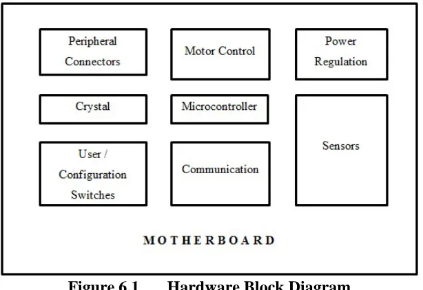
Similar to the mechanical design, the hardware design benefits from an iterative approach that moves from the evaluation board, to the bread board, and to the final PCB. This allows the individual components and hardware blocks to be verified before final integration. Essential configuration aspects of the microcontroller are covered in this chapter specifically targeting the STM32F4. Knowledge of these configurations are required in order to correctly layout the components. Other microcontrollers will have similar conventions especially concerning crystal selection. The power system, motor control, proximity sensors, and communication modules are also covered. These can be transported to other designs that do not use the STM32F as long as the MCU has the required hardware blocks. Figure 6.1 shows the high level view of the microcontroller and underlying hardware modules.
6.1 Microcontroller Configuration
During the hardware design, it is critical to understand how the microcontroller will boot and what it will use as a clock source. Some MCUs will have multiple boot mode and clock source options. Other more advanced MCUs such as the STM32F4 have many options. These options will determine the layout and supporting components. 6.1.1 Boot Modes
One of the very first operations of the STM32F4 is to jump to a particular
memory location. The STM32F4 has a sophisticated bootloader integrated into the chip. This bootloader allows the system to boot from different regions of memory. At startup, boot pins are used to select one out of three boot options:
1) Boot from user Flash 2) Boot from system memory 3) Boot from embedded SRAM
Table 6.1 STM32F4 Boot Modes
BOOT1 BOOT0 Boot Mode Description
x 0 User Flash Memory User Flash is selected as
the boot space
0 1 System Memory System memory is selected
as the boot space
1 1 Embedded SRAM Embedded SRAM is
selected as the boot space
Table 6.2 STM32F4 Memory Map of Bootable Regions
Memory Subsection Address
Block 1 (SRAM)
Reserved 0x2002 0000 - 0x3FFF FFFF
SRAM 0x2001 C000 - 0x2001 FFFF
SRAM 0x2000 0000 - 0x2001 BFFF
Block 0 (FLASH)
Reserved 0x1FFF C008 - 0x1FFF FFFF
Option Bytes 0x1FFF C000 - 0x1FFF C007
Reserved 0x1FFF 7A10 - 0x1FFF 7FFF
System memory + OTP 0x1FFF 0000 - 0x1FFF 7A0F
Reserved 0x1001 0000 - 0x1FFE FFFF
CCM data RAM 0x1000 0000 - 0x1000 FFFF
Reserved 0x0810 0000 - 0x0FFF FFFF
Flash 0x0800 0000 - 0x080F FFFF
Reserved 0x0010 0000 - 0x07FF FFFF
Alias to Flash, system memory or SRAM
depending on BOOT pins
0x0000 0000 - 0x000F FFFF
6.1.2 Clock Source
The STM32F4 can use 3 different sources for its system clock; the High Speed Internal (HSI), High Speed External (HSE), or the Phase Locked Loop (PLL). Note that the PLL requires either the HSI or HSE clock. In a way, this means there are actually 4 clock sources; the HSI by itself, the HSE by itself, the PLL driven by the HSI, or the PLL driven by the HSE. Table 6.3 shows these clock sources and the possible speeds
to both select the clock source and to check the status of which clock source is actually being used since there are fall back mechanisms in the event one of the clock sources fails [23].
Table 6.3 Clock Options and Associated Speeds
Source Min Max Unit
HSI
(standalone)
16 16 MHz
HSE
(standalone)
4 26(1) MHz
PLL
(using either HSI or HSE)
24 168 MHz
Choosing which clock source to use depends on the target application and
environment where the MCU will be used. The main reason external oscillators are used is to gain accuracy, reduce startup time, and resist changes to temperature depending on which type of external clock source is selected [24]. Anything from a simple RC circuit to another IC can be used as an external clock source. A crystal resonator resists changes to temperature better than the internal and IC-based clocks. It also has a faster startup time. Temperature changes can cause 4% of fluctuation. If this accuracy is not a critical factor, the internal oscillator can be used to save time and lower component count by 3 [18].
the HSE crystal resonator was chosen. Since low power is not of critical consideration, the maximum clock speed of 168 MHz is desired. To achieve this speed, the HSE will be used to drive the PLL, which will multiply up the HSE crystal to the targeted speed. If power consumption does become of interest, the HSE or HSI can be used in standalone mode in order to evaluate power consumption at the lower clock speeds. The clock source chosen for this application uses the PLL driven by the HSE.
Several peripheral clocks are derived from the system clock, such as the Advanced High Performance Bus (AHB), the Low Speed Advanced Peripheral Bus (APB1), and the High speed Advanced Peripheral Bus (APB2). These clocks can be adjusted using the various prescalers. A low speed internal clock (LSI) is used for the watch dog timer while an optional low speed external clock (LSE) can be used to run a Real-Time Clock (RTC).
6.1.3 Crystal Selection and Configuration
Parallel resonance crystals contain a load capacitance value in the datasheet and are the types of crystals to use for external clocks (as opposed to series resonance). These crystals require 2 loading capacitors and possibly a resistor to make them function correctly. Choosing these components incorrectly could cause damage to the oscillator or prevent startup all together. The MCU manufacturer has supplied oscillator
Table 6.4 8 MHz crystal datasheet values
Crystal ESR 𝑪𝑳 𝑪𝑶
FOXSLF/080-20 80Ω 20pF 7pF
Calculating the oscillator gain margin
Before calculating the components, the crystal specifications must be analyzed in order to determine if it will work with the microcontroller. The gain margin is used to decide this and gives a confidence level as to whether or not the oscillator will start. To calculate the gain margin, the transconductance of the microcontroller inverter (𝑔𝑚) and the critical transconductance of the crystal (𝑔𝑚𝑐𝑟𝑖𝑡) are taken as a ratio. The oscillator will theoretically start if this margin is greater than 1. Changes in temperature and other electromagnetic effects can cause this margin to drop below 1, resulting in oscillation failure. The common rule of thumb is to have this value be greater than 5 [25]. The transconductance of the microcontroller inverter (𝑔𝑚) is found in the data sheet for the STM32F4 and is represented in Equation 6.1. Equations 6.1-6.9 are derived from the manufacturers application note to calculate the correct components [26].
𝑔𝑚 = 5𝑚𝐴/𝑉 (min)
6.1 The critical transconductance of the crystal (𝑔𝑚𝑐𝑟𝑖𝑡) is calculated using Equations 6.2, 6.3, and 6.4, where 𝐹 is the crystal frequency, 𝐶0 is the shunt capacitance, and 𝐶𝐿 is the load capacitance.
6.2
𝑔𝑚𝑐𝑟𝑖𝑡 = 4 × 30 × (2𝜋8 × 10⁶)2× (7 × 10−12+ 20 × 10−12)2
6.3
𝑔𝑚𝑐𝑟𝑖𝑡 = 0.002158 = 0.221𝑚𝐴/𝑉
6.4 For correct compensation, the transconductance (𝑔𝑚) of the crystal should be larger than the critical transconductance calculated in Equation 6.4. Equation 6.5 shows that this is indeed the case.
𝑔𝑚 > 𝑔𝑚𝑐𝑟𝑖𝑡 , 5𝑚𝐴/𝑉 > 2.158𝑚𝐴/𝑉
6.5 Taking the ratio of 𝑔𝑚 𝑎𝑛𝑑 𝑔𝑚𝑐𝑟𝑖𝑡 provides the gain margin.
𝑔𝑎𝑖𝑛𝑚𝑎𝑟𝑔𝑖𝑛 = 𝑔𝑚𝑐𝑟𝑖𝑡𝑔𝑚 =0.2215 = 22.62
6.6 The oscillators gain margin is greater than 5 as recommended by the
Calculating the external load capacitors
Using an estimate that stray board capacitance (𝐶𝑠) is 10pF, Equation 6.7 solves for possible solutions to the loading capacitor values.
𝐶𝐿− 𝐶𝑠 =𝐶𝐶𝐿1∗ 𝐶𝐿2
𝐿1+ 𝐶𝐿2 = 20𝑝𝐹 − 10𝑝𝐹 =
𝐶𝐿1∗ 𝐶𝐿2 𝐶𝐿1+ 𝐶𝐿2
6.7 Solving for 𝐶𝐿1 and 𝐶𝐿2 reveals many solutions, some of which are negative or not common capacitor values. It is common practice to have the two values match. Table 6.5 shows some of the solutions to Equation 6.7.
Table 6.5 Solutions to Equation 6.7
𝑪𝑳𝟏 (𝒑𝑭) 𝑪𝑳𝟐 (𝒑𝑭)
5 -10
14 35
15 30
20 20
30 15
35 14
From Table 6.5, 20pF is the best solution for 𝐶𝐿1and 𝐶𝐿2.
𝐶𝐿1 = 𝐶𝐿2 = 20𝑝𝐹
6.8 Calculating the drive level and external resistor
given as 100uW [27]. The actual drive level that will be presented to the oscillator from the microcontroller must be calculated while the oscillator is running with the capacitors. If the drive level is less than the 100uW rating, then no additional resistor is required. If it is greater, a resistor is required in order to not damage the crystal from excessive vibration. Measuring the current flowing into the crystal is an involved process requiring additional prototyping and test equipment such as a current probe or low impedance scope probe. Fortunately, the STM32F4 data sheet provides current measurements for two different oscillators, one of which is similar in specification to the one used in these calculations (the FOXSLF/080-20). The drive level in Equation 6.9 shows that it is sending nearly 12 times less power than the maximum ratting of 100uW and therefore does not require resistor 𝑅𝐸𝑋𝑇.
𝐷𝐿 = 𝐸𝑆𝑅 × 𝐼𝑄2 = 30 × (532 × 10−6)2 = 8.5𝑢𝑊
6.9 Oscillator PCB configuration
Figure 6.2 shows the recommended PCB layout from the manufacturer with the loading capacitors 𝐶𝐿1𝑎𝑛𝑑 𝐶𝐿2 [26]. As stated above, 𝑅𝐸𝑋𝑇 is not needed. Short traces and the use of a ground plane are encouraged in order to isolate signals and reduce noise.
Observations regarding crystal selection
Going back and forth between the gain margin formula and available oscillator parameters revealed that it was very easy to have a gain margin greater than 5 if the crystal used was in the 8 MHz range or less. The STM32F4 microcontroller can use crystal values from 2-26 MHz. Available crystals have a tradeoff between effective series resistance 𝐸𝑆𝑅 and load capacitance 𝐶𝐿. Lowering the load capacitance will cause the 𝐸𝑆𝑅 to rise and vice versa. If 25 MHz is used for the oscillator the best gain margin found was 2.3. Some references suggests a margin of 2 to 3 as sufficient margin which suggests that perhaps the rule of 5 is over protective [25]. There is however no reason to use a 25 MHz clock if the PLL will be used as the clock source since any speed between 24 MHz and 168 MHz can be configured for the system clock using even a 4 MHz crystal. Since the FOXSLF/080-20 8 MHz crystal provides a margin of 22, much greater than 5, this was the chosen crystal.
6.1.4 Clock Speed Configuration
MHz or 8 MHz crystal makes for a good choice, while a 25 MHz clock makes things more difficult and provides no additional benefits unless perhaps it was used without the PLL and exactly 25 MHz was needed for an application.
To set the system clock speed, the prescalers and multipliers must be correctly configured in order to prevent overclocking or underclocking sections of the hardware. Table 6.6 describes the function of each factor and its calculated value.
Table 6.6 PLL Scale Factor Descriptions and Values
Factor Name Description Calculated Value
PLLM Division factor for the main PLL (PLL) and audio PLL (PLLI2S) input clock
8 PLLN Main PLL (PLL) multiplication factor for
VCO
336 PLLP Main PLL (PLL) division factor for main
system clock
2
The system clock can now be configured to run at the maximum frequency of 168 MHz using the PLLM, PLLN, and PLLP factors in Equations 6.10 – 6.12.
𝑃𝐿𝐿 output clock = VCO frequency/PLLP = 336/2 = 168𝑀𝐻𝑧
6.10
VCO output = VCO input × PLLN = 1MHz × 336 = 336MHz
6.11
VCO input = PLL input / PLLM = 8MHz/8 = 1MHz
factors are then written to the RCC PLL configuration register (RCC_PLLCFGR). Upon system reset, the HSI oscillator is used as the system clock until the selected clock source becomes ready as indicated by the status bits. A clock source switch is then allowed and if successful the status bits will reflect the new clock source that now uses the new
scaling factors. The main PLL configuration parameters cannot be changed once the PLL is enabled [23].
6.2 Programming/Debugging
6.2.1 Serial Wire Debug
The Serial Wire Debug (SWD) protocol is used in many ARM processors as an alternative to the traditional JTAG protocol for debugging and trace. Note that SWD still uses the JTAG protocol as its foundation but implements a two wire connection instead of six. Consequently SWD does not replace JTAG but instead provides a simpler method to connect to it. While the SWD protocol itself only requires two wires, a ground and reset line are also required in order to hold the processor in reset while being
programmed [28].
with significant overshoot. Note that this clock actually works and will allow the chip to be programmed but this is due to the additional capacitance of the probe. Once the probe is removed, the chip is no longer recognized by STLink. The actual overshoot and undershoot is so significant, there are likely double clocks happening.
For variable cable lengths ARM recommends introducing signal buffering with an inline 100Ω resistor [29]. Before considering a signal buffer it is common practice to add series resistance of a few hundred ohms in order to alter the RC time constant and
improve the rising edge of the signal. Adding 330Ω series resistors with the SWDCLK and SWDIO signals improved the signal quality and allowed the chip to be recognized by STLink. Figure 6.3 shows the original signal followed by the improved signal.
b) improved signal - added series 330Ω resistor
Figure 6.3 SWDCLK signals - 16” jumper wires
6.2.2 USART/UART/RS232
extremely rare today. Future Technology Devices International Ltd. (FTDI) makes a USB cable with an integrated chip that performs the required level shifting and USB protocol encapsulation. This cable and the STM32F4 Discovery board connect to the custom RJ45 cable, which then connects to the PCB for ease of use.
6.2.3 Combining SWD and USART into One Cable
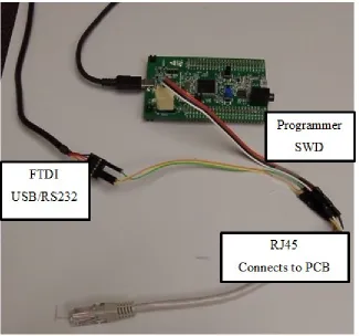
During the debug stage of an embedded system, many programming and debug cycles are done. This is a fairly straight forward process when the board can remain stationary next to the workstation. With a robotic application, the entire system needs to be disconnected, placed in the test environment, tested, and then reconnected for further adjustments to the program. Seven wires are needed to connect both the SWD and RS232 ports to the programmer and USB RS232 cable. Initially, jumper wires can be used to connect each of the appropriate pins on the board but this quickly becomes
tiresome and consumes approximately 30 seconds for each iteration. Another option is to have two separate headers, a 4 pin for the SWD and a 3 pin for the RS232. This is better but time is still taken to ensure that the polarity is correct so the total time is reduced to approximately 10 seconds. The fastest cabling solution is a single cable where polarity is solved with the shape of the connector. An RJ45 Ethernet connector has 8 pins and robust housing to ensure a correct and solid connection after many connects and disconnects, making it a suitable candidate for 2 seconds or less connection time [31].
Table 6.7 shows the pinout from the RJ45 connector to the SWD and RS232 modules.
Table 6.7 RJ45 to SWD/RS232 Pinout
RJ45 Pin Color Scheme Module Description Destination Pin
1 White/Orange RS232 RS232 GND FTDI GND
2 Orange RS232 RS232 TX FTDI RXD
3 White/Green RS232 RS232 RX FTDI TXD
4 Blue SWD GND - SWD SWD 3
5 White/Blue SWD SWDCLK SWD 2
6 Green SWD SWDIO SWD 5
7 White/Brown SWD NRST SWD 4
8 Brown UNUSED UNUSED
A custom cable is then made that breaks the connections out to the respective programmer and USB cable as seen in Figure 6.5.
6.3 Power System
Lithium Polymer (LiPo) and Lithium Iron Phosphate (LiFePO4) batteries were targeted for the power source given the high energy density, small form factor, and low cost. An initial estimate shows that at peak power consumption, the entire system could consume approximately 16 Watts of power. Typical power consumption during
operation will be significantly less since the motors are not both on at the same time all the time and the LEDs/Radio are also not on all the time. In order to measure the actual power consumption during operation, a current sense IC will be used. Table 6.8 shows the component power breakdown and then estimates the peak power.
Table 6.8 Estimated Component Max Power Breakdown
Component Quantity Voltage Used Est. Current Est. PWR
Faulhaber Motor 2 6V 1000 mA 6 W
STM32F4 MCU 1 3.3V 400 mA 1.32 W
XBEE Radio 1 3.3V 50 mA 165 mW
IR LED 3 5V 400 mA 3000 mW
FSH7773 IR LED 2 3.3V 400 mA 1320 mW
UV LED 1 3.3V 30 mA 99 mW
LED various 7 3.3V 1400 mA 4620 mW
Total 3.88A 16.524W
Given these peak estimates, the primary supply chosen for the system of
components is a 500mAh two cell (7.4v) LiPo battery with a JST connector rated for 20-30c discharge. The pack weighs 32 grams and measures 14.5mm x 31mm x 57.5mm. A similar LiFePO4 pack has also been selected but has 700mAh 6.6v rating. The
6.4 Motor Control
6.4.1 H-Bridge Circuit
A mechanism is required to control the direction and speed of the brushed DC motors. In order to provide the ability to rotate the motor shaft forward and backward, an h-bridge is commonly used. The simplest h-bridge circuit involves 4 transistors and 4 diodes arranged so that digital logic can control the direction of current flow. Additional analog circuity is required if additional features are desired, such as brake and speed control. Several integrated circuits are available that integrate one or more h-bridge circuits into a single low cost package. The TI SN754410, TI DRV8833, and Toshiba SN754410 were evaluated for this project. The SN754410 is considered a quadruple half-h driver also known as a dual full h-bridge driver. A dual full h-bridge is capable of driving 2 DC motors forward and backward independently. While the SN754410 worked well on the breadboard, it consumed too much space on the final board since it is a
through hole component. The DRV8833 initially appeared to be a valid candidate but proved to have a design that required 4 PWM inputs as compared to others that only require 2. The DRV8833 also uses a package developed by TI known as a “Power Package” or PWP. This package is considerably smaller than other h-bridge ICs but requires that the bottom center of the package be grounded to the PCB in order to maximize heat transfer. This requires that the part be re-flowed, which adds to the
6.4.2 Speed Control
In a DC motor, the armature is the current carrying mechanism that spins inside the casing in order to produce power when used as a generator or to convert power to mechanical torque via the shaft output. Equation 6.13 shows that the motor speed is proportional to the back EMF of the armature 𝑉𝐸 and is inversely proportional to the field flux 𝜙, which depends on the field excitation current [32].
𝑀𝑜𝑡𝑜𝑟 𝑆𝑝𝑒𝑒𝑑 =𝑉𝜙𝐸
6.13 Since the field flux is typically a constant, changing the back EMF is used to vary the speed of the motor. The back EMF is the opposing force of the motor that is
overcome by the applied EMF delivered by a power source. Considering the total voltage drop across the motor as the back EMF plus the drop due to the current and internal resistance of the motor, it is clear that varying the armature voltage will consequently vary the motor speed.
𝐴𝑟𝑚𝑎𝑡𝑢𝑟𝑒 𝑉𝑜𝑙𝑡𝑎𝑔𝑒 = 𝑉𝐸+ 𝐼𝐴𝑅𝐴
6.14 The motor of interest is rated for 6V but it has been determined through
experimentation that supplying 5V to the motor still produces enough speed for
controlled using a microcontroller. The frequency of this square wave is adjustable and often in the range of a few kHz to 10 kHz+ depending on the motor.
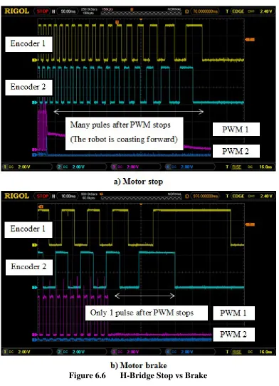
6.4.3 Stopping vs Braking
Most h-bridge ICs provide the ability to brake the DC motor as opposed to simply cutting power to it. This is often called “short braking” because shorting the terminals of a motor will dissipate the generated electrical energy into the armature. In order to not exceed the electrical ratings of the motor, a resistor is placed across the armature
6.5 Proximity Sensors
6.5.1 LTE-302/LTR-301 IR Emitter and Detector
The LTE-302 is a 940nm IR emitter built into a square side emitting package. It is spectrally and mechanically matched to work with its counterpart the LTR-301 phototransistor. The side looking package reduces, if not eliminates, the need to baffle the detector from the emitter. The phototransistor is a NPN type Bipolar Junction Transistor (BJT). NPN is not an acronym. It instead represents the configuration of silicon with respect to the Emitter (N-Type semiconductor), Base (P-Type
semiconductor), and Collector (N-Type semiconductor). An N-Type semiconductor has a spare negatively charged electron while the P-Type has a spare positively charged electron or “hole.” In a NPN phototransistor, current is allowed to flow once enough voltage is built between the base and emitter via the photoelectric effect. As a result, no current flows when it is dark, and the resistance across the emitter and detector is high. As infrared light is introduced to the sensor, more current flows from collector to emitter, and the resistance between collector and emitter is reduced.
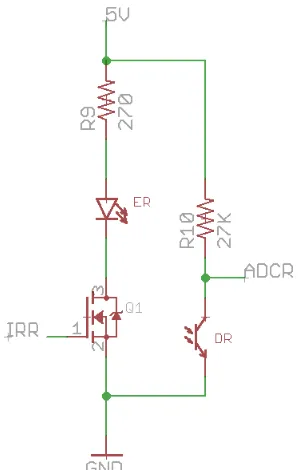
When nothing is in front of the phototransistor, only the ambient infrared will be detected and this base level can be marked in firmware as the obstruction free value. In the same way, an object is placed in front of the detector and its digital value is marked as the obstruction nearby value. Figure 6.7 shows the emitter with a 270Ω current limiting resistor and the detector acting as the second resistor in a voltage divider. IRR enables the circuit and ADCR is sampled by the MCU’s ADC port. Note the importance of the 27k resistor in the voltage divider. The MCU’s ADC voltage supply is allowed to go up to 5V, allowing voltage measurements up to 5V, but in this design it was configured to use 3.3V. Since 3.3V is the maximum value that the MCU is configured to measure, the voltage divider should be configured to output 0-3.3V.
Figure 6.7 LTE-302 / LTR-301 IR Emitter / Detector Circuit
6.5.2 SFH 7773 Integrated IR Emitter and Detector