Ann. Geophys., 25, 1509–1517, 2007 www.ann-geophys.net/25/1509/2007/ © European Geosciences Union 2007
Annales
Geophysicae
Lightning stroke distance estimation from single station observation
and validation with WWLLN data
V. Ramachandran, J. N. Prakash, A. Deo, and S. Kumar
School of Engineering and Physics, University of the South Pacific, Suva, Fiji
Received: 3 December 2006 – Revised: 2 June 2007 – Accepted: 27 June 2007 – Published: 30 July 2007
Abstract. A simple technique to estimate the distance of the lightning strikesd with a single VLF electromagnetic wave receiver at a single station is described. The technique is based on the recording of oscillatory waveforms of the elec-tric fields of sferics. Even though the process of estimat-ingd using the waveform is a rather classical one, a novel and simple procedure for findingdis proposed in this paper. The procedure adopted provides two independent estimates of the distance of the stroke. The accuracy of measurements has been improved by employing high speed (333 ns sam-pling rate) signal processing techniques. GPS time is used as the reference time, which enables us to compare the calcu-lated distances of the lightning strikes, by both methods, with those calculated from the data obtained by the World-Wide Lightning Location Network (WWLLN), which uses a multi-station technique. The estimated distances of the lightning strikes (77), whose times correlated, ranged from∼3000– 16 250 km. When d<3500 km, the average deviation in d compared with those calculated with the multi-station light-ning location system is ∼4.7%, while for all the strokes it was∼8.8%. One of the lightnings which was recorded by WWLLN, whose field pattern was recorded and the spectro-gram of the sferic was also recorded at the site, is analyzed in detail. The deviations ind calculated from the field pattern and from the arrival time of the sferic were 3.2% and 1.5%, respectively, compared todcalculated from the WWLLN lo-cation. FFT analysis of the waveform showed that only a narrow band of frequencies is received at the site, which is confirmed by the intensity of the corresponding sferic in the spectrogram.
Keywords. Meteorology and atmospheric dynamics (Light-ning) – Electromagnetics (Guided waves) – Radio science (Atmospheric propagation)
Correspondence to: V. Ramachandran ([email protected])
1 Introduction
A technique of locating the source of lightning by a single station would markedly improve the research of atmospher-ics. In the inverse technique of interpreting the unknown spectrum of the source (i.e. the parent lightning discharge) from the received spectra at a site, one important parameter required is the distance of the stroke from the receiver. Line-of-sight “ground waves” from the stroke provide information on source characteristics. Lightning locations are also useful in providing weather data over wide regions, in climate stud-ies and for meteorological forecasting. It is well established that lightning produces a wide spectrum of electromagnetic radiation with peak spectral density in the VLF (3–30 kHz) band centered∼10 kHz. The lightning-generated VLF im-pulses (sferics) travel in the Earth-Ionosphere WaveGuide (EIWG) with very little attenuation (2–3 dB/Mm) (Wood and Inan, 2002). This band of spectrum is studied in this paper.
The quest of lightning location can be solved by means of multi-station or single-station techniques. Multi-station techniques are the most accurate and several systems have been developed in the past decades. The different systems available for lightning remote sensing have complementary levels of detail, range, and application. To summarize a few: Lightning-Mapping Arrays (Rison et al., 1999; Thomas et al., 2000), UK Met Office VLF system (Lee, 1986a, b, 1989), the U.S. National Lightning Detection Network (Cummins et al., 1998), the Los Alamos Sferic Array (LASA) (Smith et al., 2002), the Europe ZEUS system (Chronis and Anag-nostou, 2003), World-Wide Lightning Location Network (WWLLN) (Dowden et al., 2002; Lay et al., 2005; Rodger et al., 2005). Lightning Imaging Sensor (LIS) aboard the TRMM satellite provides data on global lightning activity but with less detail (Boccippio et al., 1999).
1510 V. Ramachandran et al.: Lightning stroke distance estimation received on an oscilloscope at a station, Hepburn (1960)
es-timated the distance of the lightning strikes. In this analysis, the smooth oscillatory waveform was assumed to be quasi-periodic. For a stroke distance ofd and lower ionosphere heighth, the quasi-periodsτ and their delay timesT were predicted to be related as
T = d
"
1 − τ2c2
.
4h2
−1/2
− 1
# ,
c. (1)
A family of delay vs. quasi-period curves (T–τ plots) were drawn for different values of d with h=85 km. By curve-fitting the experimental T and τ plots with the theoretical plots, the distance of the stroke was estimated. Hepburn (1960) reported that the theoretical and experimental plots had a deviation of∼17.5% when meand<3200 km, with an increase in the deviation as the distance increased. A similar approach has been used by Rao (1968), but withhas 80 km, and reported±10% to±15% deviation in the two plots.
The separationτbetween the onset of the VLF component and the first maximum of the “slow tail” is derived by Wait (1962, p 314) and is given by
τ = 0.09
d
2h√ωr
+δ12
2
, (2)
where ωr is the conductivity parameter of the ionosphere
andδ is an approximately constant term corresponding to the pulse width at the source impulse. By measuring τ, a real-time distance estimation of lightning strikes using sfer-ics recordings at a single station has been developed (Sao and Jindoh, 1974).
Using the general expression for the phase of thenth mode derived by Wait (1962, p 290), Rafalsky et al. (1995) ob-tained the expression for the phase of thenth mode at a re-ceiver at a distancedas
Fn=kd(Sn−1), (3)
whereSn=
h
1− n πk h2i
1 2
andk=2π f/c. Assumingh as 86.9 km with the frequency interval restricted to 1.8–3.2 kHz (mode 1), the phase vs. frequency spectrum for the first or-der mode was theoretically computed for differentd values and compared with the experimental phase plot of the Hz
field. The discrepancy in the estimation ofd was reported to be between 5 to 7% whend was in the range of 3000 to 3500 km.
When the lightning flashes are strong enough, they pro-duce experimentally detectable Shumann resonance patterns. It has been reported (Boccippio et al., 1998) that by measur-ing the ELF transients and computmeasur-ing the range-dependent complex wave impedance, lightning locations were detected; however, the error was 0.5–2.0 Mm. Price et al. (2002) reported an ELF/VLF method for globally locating sprite-producing lightning. The VLF magnetic components were used to find the azimuth while the wave impedance of the
ELF components gave the distance of the stroke. For posi-tive cloud-to-ground lightning they have reported a mean er-ror of 1.6%. In the single station lightning location system reported by Itano et al. (2006), sequential pulses appearing on the waveform of each VLF sferic were used to estimate the distance to the corresponding lightning return stroke. The location error was reported as∼10%.
In this paper, we describe a novel, simple and cost effective system to estimate the distance of the lightning strikes with a single VLF electromagnetic wave receiver at a single sta-tion. Our technique is based on the observation of oscillatory waveforms of the sferics fields. A simple procedure for find-ingdusing the period and the delay extracted from the quasi-periodic waveform of the electric field received at the station is described in this paper. By employing sophisticated signal processing techniques, we also try to improve the accuracy for measurement of the sferics’ waveform arrival times. The waveforms were recorded with respect to GPS times, which are then correlated with stroke times recorded by WWLLN, which is a multi-station location system. A recent compara-tive study of LASA–WWLLN by Jacobson et al. (2006) have shown a very good correlation (15–20 km) of lightning loca-tion. The distances calculated using the times recorded from the waveforms are then correlated with the distances calcu-lated from WWLLN locations and stroke times. The dis-tances so calculated are then used to correlate with the sferics in the spectrogram recorded at the site.
2 Theory
The current in a typical lightning return stroke reaches its peak value in ∼2µs and decays to a half peak in∼40µs (Uman, 1987, p 77). This results in a short pulse of elec-tromagnetic radiation ∼100µs covering a very wide band of frequencies. Lee (1989) points out that effectively all the VLF power from the first return stroke comes from the lowest 2 km, which is a small fraction of a wavelength in the VLF band (10–100 km), so the source of the VLF radiation is a short current element. Thus, we can assume that the phase of all the VLF Fourier components of the current is the same so that the initial phase is the same for all the VLF Fourier components of the radiated electric field.
Consider TM mode propagation of the sferics in a sim-ple form (parallel plate) of EIWG. Assuming the cutoff fre-quency of the EIWG asfc, the phase constant for the Fourier
component of frequencyf propagating in the waveguide is (Rao, 2004, p 552)
k=ω c
"
1−
f
c f
2#
1 2
, (4)
and the phase velocity is vp=
ω
V. Ramachandran et al.: Lightning stroke distance estimation 1511 Dowden et al. (2002) assumed the constant initial phase
an-gle of the individual Fourier components as zero, and ex-pressed the waveform at a distancedfrom the source for the different frequencies asA(ω)coshωt−d
vp
i
, whereA(ω) is a weighting function given by cos2πω−ωa
2ωr
, whereωa
is the frequency of peak spectral density (10 kHz), andωr
is chosen to correspond to the bandwidth. Assumingωr as
14 kHz so that the half power frequencies are 5 and 19 kHz, which is typical of sferic spectra, they then synthesized the sferic waveform at different distances d by summing 100 waveforms. The plots showed that the wave packet expands with distanced.
On a conventional oscilloscope, triggered by the incoming pulse, the trace of the sferic field will appear as the trace in Fig. 1. (This trace was obtained by passing one of the wave-form data recorded on the picoscope through a low pass filter available in the MATLAB program.) We can interpret the trace as follows: the high frequency Fourier components of the sferic field (ffc), all traveling with a speedc, arrive at
the same timet0(with respect to the lightning stroke time), at
a receiver a distancedfrom the source. The lower frequency components of the sferics field (f >fcbut close tofc), will,
however, undergo dispersion. If we consider a narrow band of signals in this region, they superimpose, giving rise to a quasi-periodic wave, and travel with the group velocityvg.
For frequency componentsf close to the cutoff frequency, the group velocityvg=dωdk. Using Eq. (4)
vg=c
"
1−
f
c
f
2#
1 2
. (6)
The group velocities progressively decrease as f approach fc. The synthesized waveform reported by Dowden et
al. (2002) ford>1000 km was very similar to the trace from A–K of Fig. 1.
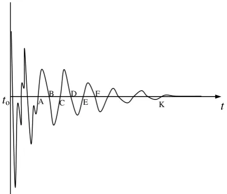
In the treatment presented in this paper, the oscillatory por-tion of the sferic field pattern is considered to be composed of quasi-periodic waves of different frequencies. In Fig. 1, the portion of the waveform starting from A to K is oscil-latory. We assume that the frequency of the quasi-periodic wave A–C is
f = 1
TC−TA
(7) and is received at a time (to+TB)with respect to the stroke
time. Similarly, the quasi-periodic wave B–D of frequency f=1
(TD−TB)is received at a time (to+TC), etc. In
gen-eral, the timeTB,TC with respect to the start of the trace is
represented asT in what follows. Note thatf is greater than the cutoff frequencyfc of the EIWG. For a group of waves
around frequencyf (>fc), the time of arrival at the site is
related as t0+T =
d vg
, (8)
20
Figure 1 Typical waveform of sferic field pattern.
A B C D E F K
t
t
oFig. 1. Typical waveform of sferic field pattern.
wheret0=dc. Substituting fortoandvg, T = d
c
1
1−fc
f
2
1 2
−d
c. (9)
Equation (9) is identical to Eq. (1) proposed by Hepburn (1960), wherec/(2h)is the cutoff frequencyfcof the EIWG
andτis the period (=1/f )of the quasi-periodic wave. It is in-teresting to note that when the phase difference is computed after a timeT, it is identical to Eq. (3) proposed by Rafalsky et al. (1995).
From Eq. (9) it is seen that in a graph of T vs.
1−fc
f
2−
1 2
, the slope is dc and the intercept is−d
c, thus
providing two independent methods of calculating the source distance.
3 Experimental setup
University of the South Pacific, Fiji (Lat. 18◦080S, Long. 178◦270E) is one of 28 Universities/Institutions which par-ticipate in the global lightning detection program under WWLLN. This network uses the Time Of Group Arrival (TOGA) method for lightning location. Detailed theory of the TOGA principle and a description of the measurement method can be found in Dowden and Rodger (2001), Dow-den et al. (2002).
[image:3.595.312.545.63.262.2]1512 V. Ramachandran et al.: Lightning stroke distance estimation
21
-1 -0.5 0 0.5 1 1.5
0
0.
5
1.
0
1.
5
2.
0
2.
5
time (ms)
am
pl
itu
de
(v
) c
-1.5 -1 -0.5 0 0.5 1 1.5
0
0.
5
1.
0
1.
5
2.
0
2.
5
time (ms)
am
pl
itu
de
(v
) b
-2 -1.5 -1 -0.5 0 0.5 1 1.5 2 2.5
0
0.
5
1.
0
1.
5 2.0
2.
5
time (ms)
am
pl
itu
de
(v
) a
[image:4.595.50.287.59.504.2]22
Figure 2. Electric fields of sferics registered in September, 2006.
a) 13:01:06 LT – 01:01:06 UT (Sep 28), b) 19:00:28 LT – 07:00:28 UT (Sep 8), c) 23:00:06 LT – 11:00:06 UT (Sep 3), d) 03:04:04 LT – 15:04:04 UT (Sep 23).
-1.2 -1 -0.8 -0.6 -0.4 -0.2 0 0.2 0.4 0.6 0.8 1
0
0.
5
1.
0
1.
5 2.0 2.5
time (ms)
am
pl
itu
de
(v
)
d
Fig. 2. Electric fields of sferics registered in September, 2006. (a) 13:01:06 LT – 01:01:06 UT (28 September), (b) 19:00:28 LT
– 07:00:28 UT (8 September), (c) 23:00:06 LT – 11:00:06 UT (3 September), (d) 03:04:04 LT – 15:04:04 UT (23 September).
mounted on top of the roof of a two-storey building. The GPS antenna is also fitted on the roof about 10 m from the VLF antenna. The VLF output of the antenna is first am-plified by a VLF preamplifier which has two parallel out-puts. The peak output voltage of the preamplifier is 10 V. The amplifier has a distributed RC filter which has attenua-tion in dB proporattenua-tional to the square root of the frequency. (i.e.∼6 dB at 40 kHz, and∼48 dB at 2.5 MHz). The GPS antenna output is connected to a splitter which has two out-puts. One of the outputs of the preamplifier and one from
the splitter are fed into a “service unit”, which contains the VLF sensor and the GPS “engine”, whose output is fed to the sound card of a PC(1) used for TOGA measurement. A de-tailed description of the experimental setup used at the site is given in Ramachandran et al. (2005). The processing centre of WWLLN at University of Seattle, Washington provides the participating Institutions with monthly data of lightning locations and the stroke times (accurate toµs), on a CD. Us-ing the WWLLN program which is installed on the PC(1) at our station we can simultaneously record the spectrogram of the sferics received, and these can be later extracted using MATLAB codes.
The other output of the preamplifier and the GPS is used to record the waveforms of the sferics. This second output of the preamplifier is fed to a high speed picoscope (Pico ADC 212/3), which has a sampling rate of 3 MS/s, with an accuracy of 1%. The picoscope has the provision of setting a threshold voltage on the rising edge to trigger the recording. The output of the picoscope is connected to another PC(2) and the GPS was connected to the COM 1 port of PC(2). The sferic waveforms and their spectrograms were recorded during the first 5 min of every hour of the day.
4 Results and discussion
4.1 Sferic field recording and analysis
V. Ramachandran et al.: Lightning stroke distance estimation23 1513
Figure 3. Picoscope output of the sferic waveform. (28/9/2006, 18:01:04 LT – 06:01:04 UT) -1.5
-1 -0.5 0 0.5 1 1.5
0
10
00
00
20
00
00
30
00
00
40
00
00
50
00
00
60
00
00
70
00
00
80
00
00
90
00
00
10
00
00
0
time (ns)
A
m
pl
itu
de
(V
)
[image:5.595.313.546.63.144.2]X
Fig. 3. Picoscope output of the sferic waveform (28 September
2006, 18:01:04 LT–06:01:04 UT).
24
Figure 4. The power spectrum of the sferic. 0
2 4 6 8 10 12 14 16
0 20 40 60 80 100
Frequency (kHz)
P
ow
er
28.2
5.5 21.3
Fig. 4. The power spectrum of the sferic.
Figures 2a–d show typical waveforms recorded at differ-ent times of the day and on differdiffer-ent days. The times and days corresponding to the waveforms in Fig. 2 corresponded with WWLLN detection (detail discussion in Sect. 4.2). The traces show that, in the oscillatory region of the field, the wave pattern expands with time. In all the traces analyzed (77), the number of full waves varied from 4 to 8, more than 70% of them having at least 6 full waves. The gen-eral quasi-periodical form (including noise) did not have any dependence on the sferics’ arrival time or the distances they have travelled. For detail analysis presented in this section, a waveform was selected whose time corresponded to the de-tection by WWLLN, and also we were able to record the spectrogram of the sferics corresponding to the lightning. Figure 3 shows the waveform recorded on 28 September 2006, at 06:01:04 UT, which is 18:01:04 LT. The “noise”-like pattern after 1.0 ms continued up to∼2.75 ms.
FFT analysis of the entire waveform shown in Fig. 3 was performed with MATLAB and the power spectrum, in arbi-trary units, is shown in Fig. 4.
The VLF region of the sferic showed waves with peak powers ∼9.5 kHz and ∼10.3 kHz, with two more groups of waves ∼15.8 and ∼18 kHz, but with reduced power. The power spectrum starts at ∼5.5 kHz and dies off after 28.2 kHz, with a dip in power at 21.3 kHz. Small peaks at higher frequencies (∼46.9, 62.3, 78.5 kHz) were also ob-served. When the FFT analysis was repeated for the
wave-25
y = 0.0157x - 0.0158
R2 = 0.9762
0 0.0001 0.0002 0.0003 0.0004
1.0100000 1.0150000 1.0200000 1.0250000 1.0300000 1.0350000
c/vg
T
(s
)
[image:5.595.51.285.64.167.2]Figure 5. Graph of quasi-wave period vscvg.
[image:5.595.51.286.225.346.2]Fig. 5. Graph of quasi-wave period vs.c vg.
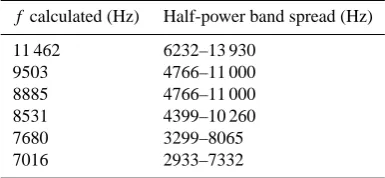
Table 1. Frequency and half-power band spread of the quasi-periodic waves.
f calculated (Hz) Half-power band spread (Hz)
11 462 6232–13 930
9503 4766–11 000
8885 4766–11 000
8531 4399–10 260
7680 3299–8065
7016 2933–7332
form from the beginning to the point marked X in Fig. 3, the minor peaks appearing above 60 kHz almost vanished and the peak at 46.9 kHz reduced, confirming that the initial por-tion of the waveform carried the VLF signal.
For the waveform in Fig. 3, the frequencies of the quasi-periodic waves were calculated using Eq. (7). To calculate the frequency of the quasi-periodic wave, the time of crossing thet axis was determined by the MATLAB program. FFT analysis was also done for each of the quasi-periodic waves, and their half-power bandwidths were calculated. The results are summarized in Table 1. The calculated frequencies of the quasi-periodic waves are within the half-power band spread of the FFT. This is to be expected since each of the quasi-periodic waves given in the trace are assumed to be due to the superposition of many waves whose frequencies are around the calculated frequency.
Considering more than 450 tweeks at our station during a two-year study (2003–2004), Kishore et al. (2005) showed that the nighttime cutoff frequency for the fundamental mode varied between 1.6–1.8 kHz. Figure 5 shows the plot of mea-sured T against
1−fc
f
2−
1 2
=cv
g
, wheref is the frequency calculated from the wave pattern andfc was
as-sumed to be the mean cutoff frequency 1.7 kHz.
[image:5.595.330.523.226.315.2]1514 V. Ramachandran et al.: Lightning stroke distance estimation
Table 2. Sample WWLLN data.
eastward
Date and Time UT Latitude Longitude No. of
stations
28 Sep 2006, 06:01:03.436155 7.1199 110.4846 5
28 Sep 2006, 06:01:04.908366 24.3935 128.7729 7
28 Sep 2006, 06:01:07.705695 36.353 22.5975 6
westward
28 Sep 2006, 06:01:02.947788 18.7792 73.9523 6
28 Sep 2006, 06:01:16.737547 7.2238 79.0363 8
4.2 WWLLN data and distance estimation
The WWLL Network confirms that lightning has occurred when 5 or more stations have recorded the sferic (Rodger et al., 2006). WWLLN provides the participating stations with CDs, every month, which when read with MATLAB, give the date, the time of the lightning strike in UT, accu-rate up to a µs with respect to GPS time, the coordinates of the stroke and the number of stations that recorded the sferic. As explained in Sect. 4.1, when the data of the wave-form is retrieved from PC(2), the beginning of the file is displayed up to s (PC time). The computer clock of PC(2) was synchronized with the GPS clock. To identify the loca-tion of the lightning, on 28 September 2006, over the entire globe, MATLAB codes were written to analyze the WWLLN records for latitude −90◦ to +90◦, longitude 0◦ to +180◦ (eastward) and −180◦ to 0◦ (westward). The WWLLN records were then manually analyzed to identify any light-ning detection around the time the waveform of Fig. 3 was recorded (06:01:04 UT). The time interval for the search was ±1 s of the UT. The section of the data on 28 September 2006 around 0.6:01:04 UT is shown in Table 2. The last column in Table 2 refers to the number of stations that recorded the sferic impulse. We observe that a lightning strike has oc-curred at 06:01:04.908366 (UT). The WWLLN record does not show any other lightning around this time (accurate to s). This leads us to conclude that the field pattern recorded at our station may have been due to the lightning strike at 06:01:04.908366 (UT) at Lat. 24.3935, Long. 128.7729, as estimated by the WWLLN.
The great circle distance between the identified location and the measurement site was calculated using the website http://www.movable-type.co.uk/scripts/LatLong.html. This program uses the “Haversine” formula to calculate the dis-tance. The calculated distance using the location was 5165 km. The distances calculated using the approach we adopted in this paper was from the slope 4981 km and from the intercept 5021 km. The average deviation ind calculated from the slope and the intercept, compared to that calculated
26
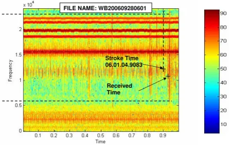
Figure 6. Spectrogram display of sferics received in 1s and the colour chart.
Stroke Time 06.01.04.9083
Received Time FILE NAME: WB200609280601
Fig. 6. Spectrogram display of sferics received in 1s and the colour
chart.
from WWLLN coordinates, is ∼3.2%. For the stroke cor-responding to the time 06:01:03.436155 the distance calcu-lated using the coordinates was 7960 km, hence this was dis-regarded.
4.3 Spectrogram recording and analysis
The WWLLN program for recording the TOGA was used to simultaneously record the VLF data, via a separate sound card, to give the spectrogram of the sferics. A program was written to start recording the VLF sferic data exactly at the hour and to record for 5 min, and then to repeat the steps every hour. A one-minute record of the data will be stored in a file of 11 MB, thus five files will be created in the 5 min. When one of these files is analyzed using MATLAB codes, it will show 60 spectrograms, each of 1 s in duration. If the sferic corresponding to the lightning that produced the field pattern of Fig. 3 has been recorded in the spectrogram, it should appear after the stroke time 06:01:04.908366 (UT), due to the travel time delay. The spectrogram which was recorded at 06:01:04 on 28 September 2006 was extracted from the files and is shown in Fig. 6. Note that 06:01:04 is the start time of the spectrogram. In the spectrogram, the stroke time is indicated by a vertical dashed line. It can be seen that 2 sferics appear after the stroke time.
V. Ramachandran et al.: Lightning stroke distance estimation 1515
27
Figure 7. Spectrogram showing tweeks.
FILE NAME: WB200609190902
Fig. 7. Spectrogram showing tweeks.
The power spectrum in Fig. 4 shows that the limits of the VLF spectrum are∼5.5 and∼28.2 kHz, with a dip in power appearing at 21.3 kHz and an appreciable amount of energy lies between∼6 to 20 kHz. The very strong sferic adjacent to the one we have identified (+ sign) had appreciable en-ergy below 5 kHz and above 24 kHz (which is the limit of the spectrogram). Therefore, we conclude that the sferic marked with + sign was the sferic corresponding to the field pattern recorded in Fig. 3. The time of arrival of the sferic (marked with +) is 06:04:01.92533 UT. By taking the WWLLN stroke time and the arrival time of the sferic at our site, the distance it has traveled is∼5090 km, which is in good agreement with the distance calculated earlier (5165 km) with the WWLLN location. The deviation indcalculated, compared to that cal-culated from WWLLN coordinates, is∼1.5%. The arrival time of the second sferic gives d=9080 km, which is very large compared to thed calculated using the location coor-dinates. An explanatory note on the sferics: 1) even though there are many sferic lines on the spectrogram in this 1-s win-dow, no lightning was recorded by WWLLN. As said ear-lier, WWLLN confirms a strike only when 5 or more stations record the sferic. 2) It has been reported (Jacobson et al., 2006) that the threshold current for detection by WWLLN is high thus the detection efficiency is low; hence, it may be that these sferics were not recorded at other stations. The lower frequency of the sferic, which is seen in the spectro-gram, does not go up to the cutoff frequency of the EIWG. This is because the intensities of the fields have died off.
A tweek shown in Fig. 7 was recorded on 19 Septem-ber 2006 at 09:02:39 (UT). From the spectrogram, we es-timate that the cutoff frequencies of the fundamental mode as∼1.7 kHz, which is thefc used in our calculations. The
cutoff frequencies of the higher modes are ∼3.4 kHz and ∼5.2 kHz, respectively. The waveform was poor to estimate
[image:7.595.311.545.63.160.2] [image:7.595.51.285.63.259.2]28
[image:7.595.312.543.202.412.2]Figure 8 Variation of deviation with distance dw.
Figure 8 Variation of deviation with distance dw. 0.00
0.05 0.10 0.15 0.20 0.25 0.30
31
60
34
23
38
59
41
43
44
69
46
77
61
81
65
64
67
85
69
00
71
89
72
76
75
80
80
47
83
54
89
19
97
57
10
67
0
11
44
0
16
25
0
dw (km)
re
la
tiv
e
de
vi
at
io
n slope
intercept
Fig. 8. Variation of deviation with distancedw. 29
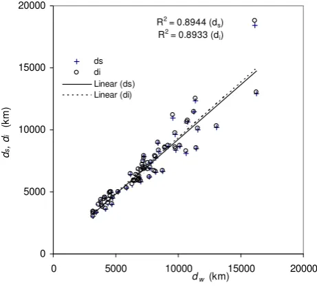
R2 = 0.8944 (d
s)
R2 = 0.8933 (d
i)
0 5000 10000 15000 20000
0 5000 10000 15000 20000
dw (km)
d
s
, d
i
(
km
)
ds di Linear (ds) Linear (di)
Figure 9. Correlation of distances ds and di with dw.
Fig. 9. Correlation of distancesdsanddiwithdw.
the distance from it. Further, the time of capture of this sferic did not correspond to the WWLLN time of detection of light-ning. The FFT of the field pattern did not show a cutoff fre-quency, as the spectrogram was extending to zero frequency. 4.4 Comparison of distances estimated by the proposed
method and WWLLN data
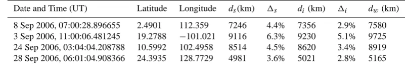
One month (1–30 September 2006) of the WWLLN data and the 5-min hourly waveform patterns recorded during this pe-riod were analyzed. It was found that 108 corresponding events were present which were distributed between day and night. The daytime cutoff frequency is not well known for this region, thus our analysis is restricted to the nighttime records. For the waveforms shown in Figs. 2b, c, d and Fig. 3 the estimated distances from the slopes of the graphs (ds)from the intercept (di)and those calculated using the
WWLLN locations (dw)are summarized in Table 3. In the
table1sand1i are the relative deviations (in %) in
estimat-ingds anddi, compared todw.
1516 V. Ramachandran et al.: Lightning stroke distance estimation
Table 3. Comparison of estimated distances of lightning strikes.
Date and Time (UT) Latitude Longitude ds(km) 1s di(km) 1i dw(km)
8 Sep 2006, 07:00:28.896655 2.4901 112.359 7246 4.4% 7356 2.9% 7580
3 Sep 2006, 11:00:06.481245 19.2788 −101.021 9116 6.3% 9230 5.1% 9725
24 Sep 2006, 03:04:04.208788 10.5992 102.4958 8514 4.5% 8620 3.4% 8919
28 Sep 2006, 06:01:04.908366 24.3935 128.7729 4981 3.6% 5021 2.8% 5165
the range of 3160–16 250 km. The deviations in the dis-tances ds anddi (i.e. dw−ds and dw−di)were both
posi-tive and negaposi-tive compared to the estimate from WWLLN data. Figure 8 shows the magnitude of the deviation (i.e. |dw−ds|dwand|dw−di|dw)in estimating the distance of
the lightning stroke using the slope and the intercept of the graph compared todw. It was noted that for 74 of the
cor-related strokes, the signs of dw−ds and dw−di were the
same. For the other three strokes,dw−ds were positive while dw−di were negative. These three strokes are identified by
the arrow marks in Fig. 8. Interestingly, the relative devia-tions in the estimated distances are small for these strokes. The averages of|1s|and|1i|were 9% and 8.5%,
respec-tively. Considering the procedures, using both the intercept and the gradient of the graphs, the average percentage devi-ation in estimating the distance is∼8.8% with respect to d calculated using WWLLN location data.
To understand the correlation between the distances cal-culated using the proposed single station technique and the multi-station technique, ds anddi were plotted against dw
and are shown in Fig. 9. The linear correlation coefficients R for both graphs were 0.95, indicating a strong correlation between the single station and multi-station methods. It is clear from the trend lines that whend is large, the corre-lation in the distance calculated using the method proposed and that calculated from coordinates predicted by WWLLN decreases.
5 Conclusion
The simple technique described in this paper provides two independent methods of estimating the distance of lightning from the sferics’ waveform at a single station. The spectral analysis of one of the waveforms shows that the frequencies below ∼5.8 kHz die off and does not show the cutoff fre-quency of the EIWG. This is confirmed by the intensity of the corresponding spectrogram. By matching the intensity of the sferics in the spectrogram with the FFT of the field pattern, the sferic which produced the waveform was iden-tified. For this identified sferic the distance estimated from the travel time is within 1.5% of the distance calculated from the WWLLN location data. Compared to the distances calcu-lated from the WWLLN locations, the deviations ind
lated from the intercepts were slightly lower than those calcu-lated from the slopes of the graphs. The distances estimated ranged from 3160 km to 16 250 km. Fordin the range 3000– 3500 km the average deviation was ∼4.7% which is lower than those reported using other VLF single station lightning location techniques. For all 77 nighttime strokes consid-ered in this study, the average deviation was∼8.8%, which is lower than many of the other reported VLF techniques. The deviations in the estimatedd increased as the distance of the stroke increase. When the distance is large, signals pass through the day/night terminator, hence the propagation conditions will change. We have assumed the nighttime cut-off frequency for the entire path, which will not hold true when waves pass through a mixed condition, whendis large. By incorporating a direction finding arrangement, using the magnetic field components of the sferic, the system could be improved as a lightning location system.
Acknowledgements. The Authors wish to acknowledge the support
of this research by the University Research Council through the grant 6C117-00.
Topical Editor F. D’Andrea thanks V. Mushtak and another anonymous referee for their help in evaluating this paper.
References
Boccippio, D. J., Wong, C., Williams, E. R., Boldi, R., Christian, H. J., and Goodman, S. J.: Global validation of single-station Schu-mann resonance lightning location, J. Atmos. Sol.-Terr. Phys., 60, 701–712, 1998.
Boccippio, D. J., Koshak, W. J., Christian, H. J., and Goodman, S. J.: Land–ocean differences in LIS and OTD tropical lightning observations, Proc. 11th Int. Conf. on Atmospheric Electricity, Huntsville, AL, National Aeronautics and Space Administration, 734–737, 1999.
Chronis, T. G. and Anagnostou, E. N.: Error analysis for
a long-range lightning monitoring network of ground-based receivers in Europe, J. Geophys. Res., 108(D24), 4779, doi:10.1029/2003JD003776, 2003.
Cummins, K. L., Murphy, M. J., Bardo, E. A., Hiscox, W. L., Pyle, R., and Pifer, A. E.: Combined TOA/MDF technology upgrade of U.S. National Lightning Detection Network, J. Geophys. Res., 10, 9035–9044, 1998.
V. Ramachandran et al.: Lightning stroke distance estimation 1517
Dowden, R. L., Brundell, J. B., and Rodger, C. J.: VLF lightning location by time of group arrival (TOGA) at multiple sites, J. Atmos. Sol.-Terr. Phys., 64(7), 817–830, 2002.
Hepburn, F.: Analysis of smooth type atmospheric waveforms, J. Atmos. Terr. Phys., 19, 37–53, 1960.
Itano, W., Nagano, I., Yagitani, S., and Ozaki, M.: Lightning lo-cation with single-station observation of VLF sferics, WAVE11-P22, 2nd Kanazawa Workshop, Japan, 2006.
Jacobson, A. R., Holzworth, R., Harlin, J., Dowden, R., and Lay, E.: Performance Assessment of the World Wide Lightning Lo-cation Network (WWLLN),Using the Los Alamos Sferic Array (LASA) as Ground Truth, J. Atmos. Ocean. Technol., 23, 1082– 1092, 2006.
Kishore, A., Kumar, S., and Ramachandran, V.: Observations of ELF-VLF sferics in the south pacific region, URSI 2005 New Delhi, 2005.
Lay, E. H.., Rodger, C. J., Holzworth, R. H., and Dowden, R. L.: Introduction to the World Wide Lightning Location Network (WWLLN), Geophys. Res. Abstr., 7, 02875, 2005.
Lee, A. C. L.: An experimental study of the remote location of lightning flashes using a VLF arrival time difference technique, Q. J. Roy. Meteor. Soc., 112, 203–229, 1986a.
Lee, A. C. L.: An operational system for the remote location of lightning flashes using a VLF arrival time difference technique, J. Atmos. Ocean. Technol., 3, 630–642, 1986b.
Lee, A. C. L.: Part B. Ground truth confirmation and theoretical limits of an experimental VLF arrival time difference lightning flash locating system, Q. J. Roy. Meteor. Soc., Part B., 115(489), 1147–1166, 1989.
Price, C., Asfur, M., Lyons, W., and Nelson, T.: An
im-proved ELF/VLF method for globally geolocating
sprite-producing lightning, Geophys. Res. Lett., 29(3) 1031,
doi:10.1029/2001GL013519, 2002.
Ramachandran, V., Kumar, S., and Kishore, A.: Remote sensing of Cloud-to-Ground lightning location using the TOGA of sferics, Atmos. Sci. Lett., 6, 128–132, 2005.
Rafalsky, V. A., Nickolaenko, A. P., Shvets, A. P., and Hayakawa, M.: Location of lightning discharges from a single station, J. Gephys. Res., 100(D10), 20 829–20 838, 1995.
Rao, M.: Some experimental results of the study of
VLF-propagation by means of sferics, J. Atmos. Terr. Phys., 30, 1667– 1676, 1968.
Rao, N. N.: Elements of Engineering Electromagnetics, Prentice Hall, New Jersy, 2004.
Rison, W., Thomas, R. J., Krehbiel, P. R., Hamlin, T., and Harlin, J.: A GPS-based three-dimensional lightning mapping system: Initial observations in central New Mexico, Geophys. Res. Lett., 26, 3573–3576, 1999.
Rodger, C. J., Brundell, J. B., and Dowden, R. L.: Location accu-racy of VLF World-Wide Lightning Location (WWLL) network: Post-algorithm upgrade, Ann. Geophys., 23, 277–290, 2005, http://www.ann-geophys.net/23/277/2005/.
Rodger, C. J., Werner, S., Brundell, J. B., Lay, E. H., Thomson, N. R., Holzworth, R. H., and Dowden, R. L.: Detection efficiency of the VLF World-Wide Lightning Location Network (WWLLN): Initial case stdy, Ann. Geophys., 24, 3197–3214, 2006, http://www.ann-geophys.net/24/3197/2006/.
Sao, K. and Jindoh, H.: Real time location of atmospherics by single station techniques and preliminary results, J. Atmos. Terr. Phys., 36, 261–266, 1974.
Smith, D. A., Eack, K. B., Harlin, J., Heavner, M. J., Jacobson, A. R., Massey, R. S., Shao, X. M., and Wiens, K. C.: The Los Alamos sferic array: A research tool for lightning investigations, J. Geophys. Res., 107(D13), 4183, doi:10.1029/2001JD000502, 2002.
Thomas, R. J., Krehbiel, P. R., Rison, W., Hamlin, T., Boccip-pio, D. J., Goodman, S. J., and Christian, H. J.: Comparison of ground-based 3-dimensional lightning mapping observations with satellite-based LIS observations in Oklahoma, Geophys. Res. Lett., 27, 1703–1706, 2000.
Uman, M. A.: The Lightning Discharge, Dover, New York, 1987. Wait, J. R.: Electromagnetic waves in stratified media, Pergamon,
New York, 1962