The inﬂuence of different PAST-based subspace trackers on DaPT parameter estimation

(1)

www.adv-radio-sci.net/10/153/2012/ doi:10.5194/ars-10-153-2012

Radio Science

The influence of different PAST-based subspace trackers

on DaPT parameter estimation

M. Lechtenberg and J. G¨otze

Information Processing Lab, TU Dortmund University, Otto-Hahn-Str. 4, 44227 Dortmund, Germany Correspondence to: M. Lechtenberg ([email protected])

Abstract. In the context of parameter estimation, subspace-based methods like ESPRIT have become common. They re-quire a subspace separation e.g. based on eigenvalue/-vector decomposition. In time-varying environments, this can be done by subspace trackers. One class of these is based on the PAST algorithm. Our non-linear parameter estimation algo-rithm DaPT builds on-top of the ESPRIT algoalgo-rithm. Evalu-ation of the different variants of the PAST algorithm shows which variant of the PAST algorithm is worthwhile in the context of frequency estimation.

1 Introduction

Parameter estimation is a common task in signal processing. It is used in DoA-applications (direction of arrival) like radar and sonar or in frequency estimation applications like radio transmission or mass spectrometry – just to name a few. We are researching parameter estimation in the context of power quality applications, i.e. finding the signal components next to the fundamental frequency to extrapolate the transmission system’s state and fault-conditions.

Next to transformation-based parameter estimation via Fourier methods like the DFT (discrete Fourier transfor-mation) and STFT (short-time Fourier transfortransfor-mation) or wavelets, there are parameter estimators based on subspace analysis. Estimators based on the separation of subspaces have advantages that justify the higher computational com-plexity: They have a significantly higher resolution not bounded by the sampling frequency and the window length and do not suffer from spectral leakage.

Common subspace-based parameter estimators are MU-SIC (multiple signal classification, Schmidt, 1986) and ES-PRIT (estimation parameters via rotational invariance tech-niques, Paulraj et al., 1985). MUSIC identifies the fre-quency components excluded from the noise subspace, ES-PRIT identifies the components from the signal subspace.

For both algorithms, noise and signal subspace have to be separated. A wide spread way to do this is to perform a de-composition into eigenvectors and separate those in noise and signal. Apart from the expensive eigenvalue decomposition, in a time-varying environment, this can also be done by effi-cient subspace trackers.

A subspace tracker can be circumscribed EV (eigenvector) updating, but this is not exactly true. The vectors generated by subspace trackers (in general) form one possible basis of the signal’s space. This basis does not have to be the EV of the correlation matrix, nor does it have to be orthogonal. The properties of the basis depend on the subspace tracker used. YAST (yet another subspace tracker, Badeau et al., 2008) and PROTEUS (plane rotation-based EVD-updating scheme, Champagne and Liu, 1998) generate an orthonormal basis, whereas PAST (projection approximation subspace tracking, Yang, 1995b) in its original form provides a basis that only approximates orthonormality over time.

Depending on the application, an orthonormal basis is not needed. To verify that our application does not require an orthonormal basis, we compared the influence of different subspace trackers all based on the mentioned PAST algo-rithm. Variants of the original PAST algorithm introduce forced orthonormality (OPAST, orthonormal PAST, Abed-Meraim et al., 2000) and additional steps for numerical stability (OPAST-PGS, PAST with pairwise Gram-Schmidt-orthogonalization, Bartelmaos et al., 2005). We also in-cluded an unrolled version of PAST reducing computational complexity (PASTd, PAST with deflation, Yang, 1995a) and – as reference – pure eigenvalue decomposition (EVD).

(2)

154 M. Lechtenberg and J. G¨otze: Influence of PAST variants on DaPT

2 Application environment

Modern energy transmission systems can be characterized by two main features. On the one hand, they were designed and constructed for a more static system state with constant 75 centralized generation – on the other hand, nowadays, they are stressed by decentralized green generation (e.g. solar, wind, biomass), economic interests (e.g. stock exchange) and cross-border transmission. Decades ago, transmission man-agement was a question of several minutes and could easily 80 be done by humans tweaking a few parameters (like the excitation of a power plant’s machine). Today’s transmis-sion grid management depends on a lot more factors and is sometimes a question of seconds. To overcome these new challenges, it is desirable to have a system of measurement units being 85 able to characterize the system state without the need of human interpretation.

The signal model describing a power transmission is com-posed of supercom-posed sinusoids:

x(n)= p X

i=1 cie2πj

·fi_fsn ₊

wawgn(n) (1)

x(n)= p X

i=1 cie2πj

·fi_fsn ₊_w

awgn(n) (2)

x(n)=A(n,f)c(n)+wawgn(n) (3)

(scalar model (1) with rankp, complex amplitudeci=aiej ϕi and noisewawgn(n); vector model (2) with window lengthN and vectorn= [n...n+N−1]; matrix-vector model (3) with N×p matrix A= [a(f1)...a(fp)], where vectors a(f )= h

e2πj·ffsn_...e2πj·f n+N−1

fs iT

). The dominating sinusoid will naturally be the fundamental frequency (50 Hz/60 Hz, de-pending on the region). Next to this sinusoid, there may be interim sinusoids. These originate in oscillations from ca-pacitances and inductances characterizing the transmission lines and routing devices triggered by changes (intended or by fault) of the net configuration. They may also be the result of not correctly synchronized/well-controlled areas of the net (interarea modes).

2.1 Database assisted parameter estimation

We have designed a database-assisted parameter estimation method (DaPT, Lechtenberg and G¨otze, 2011). This algo-rithm rates incoming parameter estimations over time and provides a noise-reduced parameter estimation with reliable rank estimation.

This database has entries for each signal component con-taining frequencyfiand (complex) amplitudeci. Additional fields hold

1. Frequency drift: this field tracks the change of the frequency estimations against the database field for threshold-based frequency field updates.

2. Phase difference: it tracks the change of the phase gra-dient as second indicator for a misestimated frequency. The phase is assumed to be constant, so a linearly changing phase estimation (based on the database’s fre-quency) indicates a mismatch.

3. Severity of frequency drift/phase difference: indicators for the prior mentioned threshold-based updating rules. 4. Quality of entry: this is the actual rating. It rates how often a frequency was part of the last estimation recur-sions. Based on that, components can be marked re-liable (i.e. present), accounted for rank estimation and output.

In every recursion, the incoming frequency estimation is mapped to the most suitable database entry. Ideally, both values match neglecting the measurement noise. For entries that have been successfully mapped, the quality is increased, for the other decreased. For the drift/difference properties, the estimation is compared to the entry’s features and expo-nentially weighted added to the field. Severity is updated like the quality mentioned before. After the drift fields have been updated, the drift’s/difference’s severity is checked whether the frequency component needs to be updated. Depending on the quality, the relevant (or reliable/present) entries are selected for output and counted for rank estimation.

2.2 Estimating parameters via rotational invariance techniques

Remembering the signal model in Eq. (3), the signal can also be described by subspaces like in

x(n)=A(n,f)c(n)+wawgn(n)=S(n)+σawgn2 I . (4) Within that equation, S(n) describes the signal subspace, which can be written as a product of the eigenvectors W(n) and the eigenvalues (on a diagonal matrix) D(n):

S(n)=W(n)D(n)W(n)H. (5)

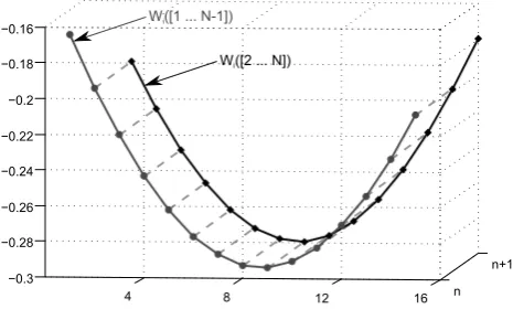
Estimating frequencies (more general: parameters) via ro-tational invariance relates to the eigenvectors of the autocor-relation matrix of the input samples. In terms of subspaces described by eigenvectors, one time-step can be described by a multiplication with a diagonal matrix8with diagonal en-triese2πj·fifs_:

S(n+1)=W(n)D(n)8W(n)H . (6) In other words, the multiplication with8is a rotation in the complex plane or a phase-shift in the time domain. This is visualized by Fig. 1.

(3)

n n+1

4 8 12 16

−0.3 −0.28 −0.26 −0.24 −0.22 −0.2 −0.18

−0.16 Wi([1 ... N-1]) Wi([2 ... N])

Fig. 1.Rotation of exemplary eigenvector from time-stepnton+1

The key idea of Esprit is to estimate the rotationΦ. Due to noise,Φwill have off-diagonal elements. So an EVD is per-formed onΦ. The frequencies can be extracted from these eigenvalues by calculating their angle. These frequencies are the input of DaPT.

145

Phase and amplitude estimation is obtained by a simple LS approach referring the signal model Eq. (3). Since time index and frequency are known, the matrixAcan be built. Together with the samples the complex amplitude can be es-timated.

150

3 Subspace Tracking

The autocorrelation matrix of the input samples is defined as Rxx=E

xxH

. The expectation value is a statistical expression that cannot be calculated for a stream of samples, but it can be estimated e.g. via exponential filtering:

Rxx≈R˜xx(n) =βR˜xx(n−1) +xxH (7)

(βis calledforgetting factor). An ordinary EVD can be ap-plied to this approximated autocorrelation matrix to generate the eigenvectors for ESPRIT. Depending on the algorithm used, this costsO(N2₎_to_O₍_N3₎_{, which is expensive}

con-155

sidering that in most casesNp. Subspace trackers real-ize the extraction of eigenvectors with computational costs in the range ofO(p2₎_{by an recursive concept of calculating}

projections and deviations to a previous calculation instead of complete decompositions.

160

This paper will focus on one branch of subspace trackers, i.e. PAST and derivations of PAST. This is in order to be able to benchmark the influence of features like orthonormality of the subspace basis on the parameter estimation without having deviations due to different calculation approaches. 165

3.1 PAST

The projection approximation subspace tracking concept (Yang, 1995b) is based on a non-constraining cost function:

J(W) =Ekx−WWHxk2=tr(Rxx)−

tr WHRxxW+tr WHRxxW·WHW (8)

(tr(...)is the trace operator). This cost function has some im-portant properties: it is minimizedif and only ifWdescribes a basis of the signal subspace; there are no more constraints regardingW, especially not orthonormality. In consequence 170

J(W)is minimized for every basis of the signal subspace, not only the basis consisting of the eigenvectors of the auto-correlation matrix.

To find the minimum of the cost functionJ, a straightfor-wardrecursive gradient-descend method is applied (step size µ). The Gradient ofJis written

5J=h−2Rxx+RxxWWH+WWHRxx

i

W (9)

(here, W is short for W(n−1)). The resulting updating equation for aWapproaching the minimum is given as fol-lows:

W(n) =W(n−1)−µ· 5J(n−1) (10)

By rearranging this equation with the projectiony=WH_x and the approximationWH_W_≈_I_{, this becomes}

W(n) =W(n−1)−µ[x(n)−W(n−1)y(n)]yH(n)

(11)

With this knowledge (Eq. (11)) and the approximation concept of the autocorrelation matrix (Eq. (7)) the cost func-tion can be reformulated as an exponentially weighted LS (least squares) problem

J0(W(n)) = n

X

i=1

βn−ikx(i)−W(n)y(i)k2 ₍₁₂₎

This is also known from adaptive filtering. The minimization of this cost function is expressed by the following equations

W(n) =Rxy(n)R−yy1(n) (13)

Rxy(n) =βRxy(n−1) +xyH (14)

Ryy(n) =βRyy(n−1) +yyH (15)

The PAST algorithm by Yang is based on the RLS ( recur-sive LS) algorithm described by the Eq. (13) and the inver-175

sion ofRxy. Whereas theWin the first definition ofJ(Eq. (8)) was not constrained to hold orthogonal columns but pro-duced an orthogonal solution, the reformulatedJ0(Eq. (12)) only approaches an orthogonal solution while convergence depends on SNR andβ.

180

This section shall only give the idea of PAST. An im-plementation can be found in other publications like Yang (1995b) or Abed-Meraim et al. (2000). The computational complexity is3N p+O p2, see Table 1.

Fig. 1. Rotation of exemplary eigenvector from time-stepnton+1.

eigenvalues by calculating their angle. These frequencies are the input of DaPT.

Phase and amplitude estimation is obtained by a simple LS approach referring the signal model Eq. (3). Since time index and frequency are known, the matrix A can be built. Together with the samples the complex amplitude can be estimated.

3 Subspace tracking

The autocorrelation matrix of the input samples is defined as Rxx=ExxH. The expectation value is a statistical expres-sion that cannot be calculated for a stream of samples, but it can be estimated e.g. via exponential filtering:

Rxx≈ ˜Rxx(n)=βR˜xx(n−1)+xxH (7) (βis called forgetting factor). An ordinary EVD can be ap-plied to this approximated autocorrelation matrix to generate the eigenvectors for ESPRIT. Depending on the algorithm used, this costsO(N2)toO(N3), which is expensive con-sidering that in most casesNp. Subspace trackers realize the extraction of eigenvectors with computational costs in the range ofO(p2)by an recursive concept of calculating pro-jections and deviations to a previous calculation instead of complete decompositions.

This paper will focus on one branch of subspace trackers, i.e. PAST and derivations of PAST. This is in order to be able to benchmark the influence of features like orthonormality of the subspace basis on the parameter estimation without having deviations due to different calculation approaches. 3.1 PAST

The projection approximation subspace tracking concept (Yang, 1995b) is based on a non-constraining cost function:

J (W)=Ekx−WWHxk2=tr(Rxx)− trWHRxxW

+trWHRxxW·WHW

(8)

(tr(...)is the trace operator). This cost function has some im-portant properties: it is minimized if and only if W describes a basis of the signal subspace; there are no more constraints regarding W, especially not orthonormality. In consequence J (W)is minimized for every basis of the signal subspace, not only the basis consisting of the eigenvectors of the auto-correlation matrix.

To find the minimum of the cost functionJ, a straightfor-ward recursive gradient-descend method is applied (step size µ). The Gradient ofJis written

5J=h−2Rxx+RxxWWH+WWHRxx i

W (9)

(here, W is short for W(n−1)). The resulting updating equa-tion for a W approaching the minimum is given as follows:

W(n)=W(n−1)−µ· 5J (n−1) (10) By rearranging this equation with the projectiony=WHx

and the approximation WHW≈I, this becomes

W(n)=W(n−1)−µ[x(n)−W(n−1)y(n)]yH(n). (11) With this knowledge (Eq. 11) and the approximation con-cept of the autocorrelation matrix (Eq. 7) the cost function can be reformulated as an exponentially weighted LS (least squares) problem

J0(W(n))= n X

i=1

βn−ikx(i)−W(n)y(i)k2. (12)

This is also known from adaptive filtering. The minimiza-tion of this cost funcminimiza-tion is expressed by the following equa-tions

W(n)=Rxy(n)R−yy1(n) (13)

Rxy(n)=βRxy(n−1)+xyH (14)

Ryy(n)=βRyy(n−1)+yyH . (15) The PAST algorithm by Yang is based on the RLS (recur-sive LS) algorithm described by the Eq. (13) and the inversion of Rxy. Whereas the W in the first definition ofJ(Eq. 8) was not constrained to hold orthogonal columns but produced an orthogonal solution, the reformulated J0 (Eq. 12) only ap-proaches an orthogonal solution while convergence depends on SNR andβ.

This section shall only give the idea of PAST. An im-plementation can be found in other publications like Yang (1995b) or Abed-Meraim et al. (2000). The computational complexity is 3Np+O(p2), see Table 1.

3.2 OPAST

(4)

156 M. Lechtenberg and J. G¨otze: Influence of PAST variants on DaPT

Table 1. Comparison of the algorithms computational complexities (Nwindow length andprank, noteNp).

EVD O(N2)

PAST 3Np+O(p2)

OPAST 4Np+O(p2)

OPAST-PGS 5Np+O(p2)

PASTd 4Np+O(p2)

the same cost function, but introduces an additional orthog-onalizing step. This step is informally written like W=

W(WHW)−0.5, with its brackets including the exponent called inverse square root.

This orthogonalizing step ensures an orthogonal basis (represented by W) in every time-step. This additional cal-culation is incorporated in the updating algorithm of PAST. The implementation can be found in the corresponding pub-lication. The computational complexity is 4Np+O(p2), see Table 1.

3.3 OPAST-PGS

Due to Bartelmaos et al. (2005), a problem of OPAST is its sensitivity to numerical rounding errors. These are originated in the inverse square root concept. The authors propose a pairwise Gram-Schmidt orthogonalization (OPAST-PGS) to oppose this problem.

Remembering that the recursion is indexed bynand the rank is p, two indices are defined: kn=mod(n,p) and kn+1=mod(n+1,p). With these indices, the kn+1-vector of W is made orthogonal to thekn-vector, before it is nor-malized:

wkn+1(n)=wkn+1(n)−wkn(n)w H

kn(n)wkn+1(n) (16)

wkn+1(n)=

wkn+1(n) kwkn+1(n)k

. (17)

The computational complexity is 5Np+O(p2)(Table 1). 3.4 PASTd

Another derivation of the PAST algorithm was proposed by Yang (1995a). This approach focuses on a further reduc-tion of computareduc-tional costs by unrolling the PAST algorithm. This deflation describes the sequential estimation of the prin-cipal components (or: basis-vectors) beginning with the most dominant. The most dominant is defined by the maximal (pseudo-)eigenvalue corresponding to the principal compo-nent.

The process is the same as for the original PAST, except that it is done for each vector of W separately. So, PAST is performed for the most dominant vector, then a projection

of the current data onto this vector is removed from the data vector. The current vector is now excluded and the process will be repeated for the new dominant vector. This method results in less matrix computations resulting in a computa-tional complexity of 4Np+O(p). Note that it isO(p)and notO(p2).

4 Simulation environment

The signal will always embody a 50 Hz-component (sloppy for fundamental system frequency ideally being 50 Hz or 60 Hz, depending on the region), slightly varying over time, and spontaneous, temporally present components with ran-dom parameters.

The simulation is Monte-Carlo based and performs 400 iterations, each having 20 sections. The following results are consistent and bias-free.

4.1 Signal generator

The signal generator is based on a concept of random tions. A default section has a length of 5 s. The actual sec-tions will have a length that is a small, random integer multi-ple of the default length. Each section varies the parameters (frequency, amplitude) of the fundamental component a lit-tle. For each section, a small random number of additional components is added and/or removed. In consequence, the additional components will endure a small random number of sections. If an additional component endures more than one section, its parameters are also slightly changed randomly.

The noise applied to the generated signal is based on the AWGN (additional white Gaussian noise) model and is lev-eled 20 dB.

4.2 Exemplary estimation

Figure 2a–b shows a typical estimation of such a signal. When viewing the total simulation time, no details of the estimation are observable. To get an insight into these algo-rithms, two cut-outs of typical estimations will be discussed. Since the database concept is non-linear and relies on its own statistics, especially the first estimations of a compo-nent have a high influence. Outliers from pure incoming fre-quency estimations can have high impact at first. Figure 3 shows this for – in this case – faulty initial estimations of PAST(d). When the database fields become statistically reli-able, the output values become consistent again.

(5)

M. Lechtenberg and J. G¨otze: Influence of PAST variants on DaPTMatthias Lechtenberg: Evaluation of PAST variants for DaPT 5157

50 100 150 time [s]

0 1000 2000

frequency [Hz]

50 100 150 time [s]

0 150 300

amplitude [V]

Fig. 2.A typical estimation picked from one of the simulations.

1 2

3

Fig. 3. A cut-out of a typical frequency estimation. (1) and (3) show aberrations due to erroneous parameter estimation and how they converge when estimations become reliable (here from PASTd and PAST); (2) points to the ideal dotted line and the EVD/OPAST-(PGS) estimation.

15 17 19 time [s]

1.2 1.6 phase [rad]

Fig. 4. A cut-out of a typical phase estimation. In the solid line, linearly increasing trends can be seen and the steps where DaPT reaches the threshold for phase difference severity and uses the gra-dient to correct the frequency estimation.

The solid line is not constant but linearly in-/decreasing (with steps). The gradient of this line is a hint on the deviation be-tween the true frequency and the current estimation. At the positions where steps occur, this gradient has been used to update the estimation.

270

5 Simulation Results

To summarize the results of the Monte-Carlo simulation, three cases will be presented. For the first, we measured the deviation of the frequency estimation and the theoretical

val-Fig. 5. Deviation of frequency estimation against true values, summed and averaged.

Fig. 6.Number of frequency components not found by the estima-tion per algorithm, summed and averaged.

ues from the signal generator. We summed them for all con-275

temporaneous components and averaged the sums over the simulation time and all simulations. Figure 5 presents the results.

First of all, it emerges that the differences between the dif-ferent algorithms are small. If there are findings at all, then 280

EVD has slight disadvantages and (O)PAST has slight advan-tages. EVD might suffer from the position of the exponential filtering. In EVD the autocorrelation matrix itself is expo-nentially filtered, which is indirect since notRxxbut the EV are desired. The other algorithms perform that step directly 285

on the basis of the subspace.

Also, we counted the number of frequency components that were not found by the estimator. Reasons may be (from

Fig. 2. A typical estimation picked from one of the simulations.

Matthias Lechtenberg: Evaluation of PAST variants for DaPT 5

50 100 150 time [s]

0 1000 2000

frequency [Hz]

50 100 150 time [s]

0 150 300

amplitude [V]

15 17 19 time [s]

136.0 136.1 frequency [Hz] 1 2 3

15 17 19 time [s]

1.2 1.6 phase [rad]

270

Fig. 3. A cut-out of a typical frequency estimation. (1) and (3) show aberrations due to erroneous parameter estimation and how they converge when estimations become reliable (here from PASTd and PAST); (2) points to the ideal dotted line and the EVD/OPAST-(PGS) estimation.

50 100 150 time [s]

0 1000 2000

frequency [Hz]

50 100 150 time [s]

0 150 300

amplitude [V]

1

2

3

15 17 19 time [s]

1.2 1.6 phase [rad]

270

Fig. 4. A cut-out of a typical phase estimation. In the solid line, linearly increasing trends can be seen and the steps where DaPT reaches the threshold for phase difference severity and uses the gra-dient to correct the frequency estimation.

5 Simulation results

To summarize the results of the Monte-Carlo simulation, three cases will be presented. For the first, we measured the deviation of the frequency estimation and the theoretical val-ues from the signal generator. We summed them for all con-temporaneous components and averaged the sums over the simulation time and all simulations. Figure 5 presents the results.

First of all, it emerges that the differences between the dif-ferent algorithms are small. If there are findings at all, then EVD has slight disadvantages and (O)PAST has slight advan-tages. EVD might suffer from the position of the exponential filtering. In EVD the autocorrelation matrix itself is expo-nentially filtered, which is indirect since not Rxxbut the EV

Matthias Lechtenberg: Evaluation of PAST variants for DaPT 5

50 100 150 time [s]

0 1000 2000

frequency [Hz]

50 100 150 time [s]

0 150 300

amplitude [V]

1 2

3

15 17 19 time [s]

1.2 1.6

phase [rad]

270

val-EVD PAST PASTd OPAST OPAST-PGS 0

0.005 0.01 0.015

0.02 skript6: DCsfrequency (2011-09-23 20-52)

sec

Fig. 5. Deviation of frequency estimation against true values, summed and averaged.

ues from the signal generator. We summed them for all

con-275

First of all, it emerges that the differences between the dif-ferent algorithms are small. If there are findings at all, then

280

EVD has slight disadvantages and (O)PAST has slight advan-tages. EVD might suffer from the position of the exponential filtering. In EVD the autocorrelation matrix itself is expo-nentially filtered, which is indirect since notRxxbut the EV are desired. The other algorithms perform that step directly

285

Also, we counted the number of frequency components that were not found by the estimator. Reasons may be (from Fig. 5. Deviation of frequency estimation against true values, summed and averaged.

50 100 150 time [s] 0

1000 2000

frequency [Hz]

50 100 150 time [s] 0

150 300

amplitude [V]

1 2

3

15 17 19 time [s]

1.2 1.6 phase [rad]

270

EVD PAST PASTd OPAST OPAST-PGS 0

100 200

300 skript6: NAsfrequency (2011-09-23 20-52)

sec

ues from the signal generator. We summed them for all

con-275

First of all, it emerges that the differences between the dif-ferent algorithms are small. If there are findings at all, then

280

EVD has slight disadvantages and (O)PAST has slight advan-tages. EVD might suffer from the position of the exponential filtering. In EVD the autocorrelation matrix itself is expo-nentially filtered, which is indirect since notRxxbut the EV are desired. The other algorithms perform that step directly

285

Also, we counted the number of frequency components that were not found by the estimator. Reasons may be (from Fig. 6. Number of frequency components not found by the estima-tion per algorithm, summed and averaged.

are desired. The other algorithms perform that step directly on the basis of the subspace.

(6)

1586 M. Lechtenberg and J. G¨otze: Influence of PAST variants on DaPTMatthias Lechtenberg: Evaluation of PAST variants for DaPT

0 200 400 amplitude [V]

0 2 number

Fig. 7. Summed and averaged not-found components plotted against the amplitude: EVD, PAST, OPAST, OPAST-PGS,

PASTd.

the signal’s perspecitve) a two weak amplitude or (from the statistical perspective) too high variance in the estimations. 290

The numbers are per second and include the mandatory non-hits before DaPT regards them as present (resulting in an off-set in the figure). In Fig. 6, the most significant fact is, that PASTd cannot keep up with the others. Also, EVD leaves a better mark. Both facts might be justified by the handling 295

of estimations with high variance. A high variance in the es-timations may confuse the sequential processing of PASTd. The joint cost of the serial cost functions might be higher than the cost of the (matrix-) PAST.

High variances (indicating less reliable estimations) are 300

most likely for low amplitudes (in relation to noise and domi-nant components). The last case surveys the unfound compo-nents against the amplitude, as (relative) amplitude is a good indicator for less reliable estimations. Figure 7 approves the previous results. PASTd is especially unsuitable for low am-305

plitudes which may hint high variances in estimations. All the other perform equally well with slight advantages for EVD and (O)PAST. OPAST-PGS does not seem to bring ad-vantages.

6 Conclusions

310

We have simulated the performance of different subspace trackers, based on the PAST theory, to evaluate the impact of the properties of the subspace basis presented to the ESPRIT algorithm. The estimated components supply the input of our DaPT non-linear parameter estimation post-processing. 315

The subspace’s basis of the signal generated from the (es-timated) autocorrelation matrix of the input samples is not unique. The subspace can be described by various basis’, some of them orthogonal, some even orthonormal and one of them being the signal eigenvectors of the autocorrelation 320

matrix.

The simulations have shown, that it is not necessary for the subsequent steps (ESPRIT, DaPT) to be provided with exact

eigenvectors (EVD). The basis presented to ESPRIT does not even have to be orthogonal (OPAST(-PGS)). The clas-325

sic PAST algorithm, which does not guarantee an orthonmal basis, performs as well as the variations providing an or-thonormal basis and as EVD providing actual eigenvectors.

A closer look reveals, that the sequential PASTd performs worse due to the lack of a joint cost function. The or-330

thonormal OPAST is marginally better than PAST, because the approximation WHW≈I is more accurate for really orthonormal columns ofW. The algorithm with additional pairwise Gram-Schmidt orthogonalization does not improve the results.

335

In future work, the phase- and amplitude estimation shall be investigated further, i.e. other algorithms as LS relating the signal model. Also, cooperative estimations of regionally displaced measurements shall be investigated.

Acknowledgements. This work was supported by DFG (German

340

Research Foundation).

References

Abed-Meraim, K., Chkeif, A., and Hua, Y.: Fast orthonormal PAST algorithm, IEEE Signal Processing Letters, 7, 60 – 62, doi:10. 1109/97.823526, 2000.

345

Badeau, R., Richard, G., and David, B.: Fast and Stable YAST Algorithm for Principal and Minor Subspace Tracking, IEEE Transactions on Signal Processing, 56, 3437 – 3446, doi:10. 1109/TSP.2008.925924, 2008.

Bartelmaos, S., Abed-Meraim, K., and Attallah, S.: Mobile local-350

ization using subspace tracking, in: 2005 Asia-Pacific Confer-ence on Communications, pp. 1009 –1013, doi:10.1109/APCC. 2005.1554216, 2005.

Champagne, B. and Liu, Q.-G.: Plane rotation-based EVD updat-ing schemes for efficient subspace trackupdat-ing, IEEE Transactions 355

on Signal Processing, 46, 1886 – 1900, doi:10.1109/78.700961, 1998.

Lechtenberg, M. and G¨otze, J.: Database Assisted Frequency Es-timation, in: 4th IEEE International Conference on Computer Science and Information Technology, 2011.

360

Paulraj, A., Roy, R., and Kailath, T.: Estimation Of Signal Parame-ters Via Rotational Invariance Techniques, in: IEEE Conference on Circuits, Systems and Computers, pp. 83 – 89, 1985. Schmidt, R.: Multiple emitter location and signal parameter

estima-tion, IEEE Transactions on Antennas and Propagaestima-tion, 34, 276 – 365

280, 1986.

Yang, B.: An extension of the PASTd algorithm to both rank and subspace tracking, IEEE Signal Processing Letters, 2, 179 – 182, doi:10.1109/97.410547, 1995a.

Yang, B.: Projection approximation subspace tracking, IEEE Trans-370

actions on Signal Processing, 43, 95 – 107, doi:10.1109/78. 365290, 1995b.

Fig. 7. Summed and averaged not-found components plotted

against the amplitude: EVD, PAST, OPAST, OPAST-PGS,

PASTd.

High variances (indicating less reliable estimations) are most likely for low amplitudes (in relation to noise and domi-nant components). The last case surveys the unfound compo-nents against the amplitude, as (relative) amplitude is a good indicator for less reliable estimations. Figure 7 approves the previous results. PASTd is especially unsuitable for low am-plitudes which may hint high variances in estimations. All the other perform equally well with slight advantages for EVD and (O)PAST. OPAST-PGS does not seem to bring ad-vantages.

6 Conclusions

We have simulated the performance of different subspace trackers, based on the PAST theory, to evaluate the impact of the properties of the subspace basis presented to the ESPRIT algorithm. The estimated components supply the input of our DaPT non-linear parameter estimation post-processing. The subspace’s basis of the signal generated from the (es-timated) autocorrelation matrix of the input samples is not unique. The subspace can be described by various basis’, some of them orthogonal, some even orthonormal and one of them being the signal eigenvectors of the autocorrelation matrix.

The simulations have shown, that it is not necessary for the subsequent steps (ESPRIT, DaPT) to be provided with exact eigenvectors (EVD). The basis presented to ESPRIT does not even have to be orthogonal (OPAST(-PGS)). The clas-sic PAST algorithm, which does not guarantee an orthonmal basis, performs as well as the variations providing an or-thonormal basis and as EVD providing actual eigenvectors.

A closer look reveals, that the sequential PASTd performs worse due to the lack of a joint cost function. The orthonor-mal OPAST is marginally better than PAST, because the ap-proximation WHW≈I is more accurate for really orthonor-mal columns of W. The algorithm with additional pairwise Gram-Schmidt orthogonalization does not improve the re-sults.

In future work, the phase- and amplitude estimation shall be investigated further, i.e. other algorithms as LS relating the signal model. Also, cooperative estimations of regionally displaced measurements shall be investigated.

Acknowledgements. This work was supported by DFG (German Research Foundation).

References

Abed-Meraim, K., Chkeif, A., and Hua, Y.: Fast orthonormal PAST algorithm, IEEE Signal Proc. Let., 7, 60–62, doi:10.1109/97. 823526, 2000.

Badeau, R., Richard, G., and David, B.: Fast and Stable YAST Al-gorithm for Principal and Minor Subspace Tracking, IEEE T. Signal Proces., 56, 3437–3446, doi:10.1109/TSP.2008.925924, 2008.

Bartelmaos, S., Abed-Meraim, K., and Attallah, S.: Mobile local-ization using subspace tracking, in: 2005 Asia-Pacific Confer-ence on Communications, 1009–1013, doi:10.1109/APCC.2005. 1554216, 2005.

Champagne, B. and Liu, Q.-G.: Plane rotation-based EVD updating schemes for efficient subspace tracking, IEEE T. Signal Proces., 46, 1886–1900, doi:10.1109/78.700961, 1998.

Lechtenberg, M. and G¨otze, J.: Database Assisted Frequency Es-timation, in: 4th IEEE International Conference on Computer Science and Information Technology, 2011.

Paulraj, A., Roy, R., and Kailath, T.: Estimation Of Signal Parame-ters Via Rotational Invariance Techniques, in: IEEE Conference on Circuits, Systems and Computers, 83–89, 1985.

Schmidt, R.: Multiple emitter location and signal parameter estima-tion, IEEE T. Antenn. Propag., 34, 276–280, 1986.

Yang, B.: An extension of the PASTd algorithm to both rank and subspace tracking, 9, 179–182, doi:10.1109/97.410547, 1995a. Yang, B.: Projection approximation subspace tracking, IEEE T.