R E S E A R C H
Open Access
Minimal and maximal solutions to first-order
differential equations with state-dependent
deviated arguments
Rubén Figueroa
*and Rodrigo López Pouso
* Correspondence: ruben. [email protected]
Department of Mathematical Analysis, University of Santiago de Compostela, Spain
Abstract
We prove some new results on existence of solutions to first-order ordinary differential equations with deviated arguments. Delay differential equations are included in our general framework, which even allows deviations to depend on the unknown solutions. Our existence results lean on new definitions of lower and upper solutions introduced in this article, and we show with an example that similar results with the classical definitions are false. We also introduce an example showing that the problems considered need not have the least (or the greatest) solution between given lower and upper solutions, but we can prove that they do have minimal and maximal solutions in the usual set-theoretic sense. Sufficient conditions for the existence of lower and upper solutions, with some examples of application, are provided too.
1 Introduction
LetI0= [t0,t0+L] be a closed interval,r ≥0, and putI-= [t0 -r,t0] andI=I-∪I0. In this article, we are concerned with the existence of solutions for the following problem with deviated arguments:
x(t) =f(t,x(t),x(τ(t,x))) for almost all (a.a.)t∈I0,
x(t) =(x) +k(t) for allt∈I−, (1)
where f : I × ℝ2 ® ℝ and τ :I0×C(I)→I are Carathéodory functions,
:C(I)→R is a continuous nonlinear operator and k∈C(I−). Here C(J) denotes the set of real functions which are continuous on the intervalJ.
For example, our framework admits deviated arguments of the form
τ(t,x) = sin2(x(t))t0+ (1−sin2(x(t))) (t0+L),
or
τ(t,x) =t− ∫Ix(s)ds
1 +∫Ix(s)ds
r.
We define a solution of problem (1) to be a function x∈C(I) such that
x|I0 ∈AC(I0) (i.e., x|I0 is absolutely continuous onI0) andxfulfills (1).
In the space C(I) we consider the usual pointwise partial ordering, i.e., for
γ1,γ2∈C(I) we defineg1 ≤g2if and only ifg1(t)≤g2(t) for alltÎI. A solution of (1),
x*, is aminimal(respectively, maximal) solution of (1) in a certain subset Y ⊂C(I) if
x*Î Yand the inequalityx ≤x*, (respectively, x≥x*) impliesx=x*, whenever xis a solution to (1) andxÎY. We say thatx*is the least(respectivelythe greatest) solution of (1) inYif x*≤x (respectivelyx*≥x) for any other solution xÎ Y. Notice that the least solution in a subset Yis a minimal solution inY, but the converse is false in gen-eral, and an analgous remark is true for maximal and greatest solutions.
Interestingly, we will show that problem (1) may have minimal (maximal) solutions between given lower and upper solutions and not have the least (greatest) solution. This seems to be a peculiar feature of equations with deviated arguments, see [1] for an example with a second-order equation. Therefore, we are obliged to distinguish between the concepts of minimal solution and least solution (or maximal and greatest solutions), unfortunately often identified in the literature on lower and upper solutions. First-order differential equations with state-dependent deviated arguments have received a lot of attention in the last years. We can cite the recent articles [2-7] which deal with existence results for this kind of problems. For the qualitative study of this type of problems we can cite the survey of Hartung et al. [8] and references therein.
As main improvements in this article with regard to previous works in the literature we can cite the following:
(1) The deviating argument τ depends at each momentt on the global behavior of
the solution, and not only on the values that it takes at the instantt.
(2) Delay problems, which correspond to differential equations of the formx’(t) =f(t,
x(t),x(t- r)) along with a functional start condition, are included in the framework of problem (1). This is not allowed in articles [3-6].
(3) No monotonicity conditions are required for the functionsfand τ, and they need not be continuous with respect to their first variable.
This article is organized as follows. In Section 2, we state and prove the main results in this article, which are two existence results for problem (1) between given lower and upper solutions. The first result ensures the existence of maximal and minimal solutions, and the second one establishes the existence of the greatest and the least solutions in a particular case. The concepts of lower and upper solutions introduced in Section 2 are new, and we show with an example that our existence results are false if we consider lower and upper solutions in the usual sense. We also show with an example that our problems need not have the least or the greatest solution between given lower and upper solutions. In Section 3, we prove some results on the existence of lower and upper solutions with some examples of application.
2 Main results
We begin this section by introducing adequate new definitions of lower and upper solutions for problem (1).
Notice first thatτ(t,g)ÎI=I-∪I0 for all (t,γ)∈I0×C(I), so for eachtÎI0we can define
τ∗(t) = inf
γ∈C(I)τ(t,γ)∈I, τ
∗(t) = sup γ∈C(I)
Definition 1 We say that α,β∈C(I), witha ≤ bon I, are a lower and an upper solution for problem (1) if α|I0,β|I0 ∈AC(I0)and the following inequalities hold:
α(t)≤ min
ξ∈E(t)f(t,α(t),ξ)for a.a.t∈I0, α≤γ∈inf[α,β](γ) +k on I−, (2)
β(t)≥ min
ξ∈E(t)f(t,β(t),ξ)for a.a.t∈I0, β≥γ∈sup[α,β](γ) +k on I−, (3)
where
E(t) =
min
s∈[τ∗(t),τ∗(t)]α(s), s∈[τ∗max(t),τ∗(t)]β
(s)
(t∈I0),
and [α,β] ={γ ∈C(I) :α≤γ ≤β}..
Remark 1Definition 1 requires implicitly thatΛbe bounded in [a,b]. On the other hand, the values
min
ξ∈E(t)f(t,α(t),ξ) and ξmax∈E(t)f(t,β(t),ξ),
are really attained for almost every fixed tÎI0thanks to the continuity off(t,a(t), ·) and f(t,b(t), ·) on the compact setE(t).
Now we introduce the main result of this article.
Theorem 1 Assume that the following conditions hold:
(H1)(Lower and upper solutions) There exist α,β∈C(I), with a≤ bon I, which
are a lower and an upper solution for problem (1).
(H2)(Carathéodory conditions)
(H2) - (a)For all x, yÎ[mintÎIa(t), maxtÎIb(t)]the function f(·,x,y)is measur-able and for a.a. t ÎI0,all xÎ [a(t),b(t)] and all yÎE(t)(as defined in
Defi-nition 1) the functions f(t, ·,y)and f(t,x,•)are continuous.
(H2) - (b)For all γ ∈[α,β] ={ξ ∈C(I) :α≤ξ≤β}the functionτ(·,g)is
mea-surable and for a.a. t Î I0 the operator τ(t, ·)is continuous in C(I)(equipped
with it usual topology of uniform convergence).
(H2) - (c)The nonlinear operator :C(I)→Ris continuous.
(H3)(L1-bound) There existsψÎ L1(I0)such that for a.a. tÎI0,all xÎ[a(t),b(t)]
and all yÎE(t) we have
f(t,x,y)≤ϕ(t).
Then problem (1) has maximal and minimal solutions in[a,b].
Proof. As usual, we consider the function
p(t,x) =
⎧ ⎨ ⎩
α(t), ifx< α(t),
x, ifα(t)≤x≤β(t),
β(t), ifx> β(t),
and the modified problem
x(t) =f(t,p(t,x(t)),p(τ(t,x),x(τ(t,x)))) for a.a.t∈I0,
Claim 1: Problem (4) has a nonempty and compact set of solutions. Consider the operator T:C(I)→C(I) which maps each γ ∈C(I) to a continuous function Tg
defined for eachtÎI-as
Tγ(t) =(p(·,γ(·))) +k(t),
and for each tÎI0as
Tγ(t) =(p(·,γ(·))) +k(t0) +
t
t0
f(s,p(t,γ(s)),p(τ(s,γ),γ(τ(s,γ))))ds.
It is an elementary matter to check thatT is a completely continuous opera-tor from C(I) into itself (one has to take Remark 1 into account). Therefore, Schauder’s Theo-rem ensures thatT has a nonempty and compact set of fixed points in C(I), which are exactly the solutions of problem (4).
Claim2:Every solution x of (4) satisfiesa≤x≤bon I and, therefore, it is a solution of (1) in [a, b]. First, notice that ifxis a solution of (4) thenp(·,x(·))Î [a,b]. Hence the definition of lower solution implies that for alltÎI-we have
α(t)≤(p(·,x(·))) +k(t) =x(t).
Assume now, reasoning by contradiction, that xα on I0. Then we can find
ˆ
t0∈[t0,t0+L) and ε> 0 such that α(ˆt0) =x(ˆt0) and
α(t)>x(t) for allt∈[ˆt0,ˆt0+ε]. (5) Therefore, for all t∈[ˆt0,ˆt0+ε] we have p(t,x(t)) =a(t) and
p(τ(t,x),x(τ(t,x)))∈[α(τ(t,x)),β(τ(t,x))]⊂E(t),
so for a.a. s∈[ˆt0,ˆt0+ε] we have
α(s)≤f(s,p(s,x(s)),p(τ(s,x),x(τ(s,x)))). Hence for t∈[ˆt0,ˆt0+ε] we have
α(t)−x(t) = t
t0
α(s)ds− t ˆ
t0
f(s,p(s,x(s)),p(τ(s,x),x(τ(s,x))))ds≤0,
a contradiction with (5).
Similar arguments prove that all solutions xof (4) obeyx≤bonI.Claim3:The set of solutions of problem (1) in[a,b]has maximal and minimal elements. The set
S={x∈C(I) :xis a solution of (1), x∈[α,β]}
is nonempty and compact in C(I), beacuse it coincides with the set of fixed points of the operatorT. Then, the real-valued continuous mapping
x∈S→I(x) = t0+L
t0
attains its maximum and its minimum, that is, there exist x∗,x∗∈S such that I(x∗) = max{I(x) :x∈S}, I(x∗) = min{I(x) :x∈S}. (6)
Now, if x∈S is such that x ≥ x* on I then we have I(x)≥I(x∗) and, by (6), I(x)≤I(x∗). So we conclude that I(x) =I(x∗) which, along withx≥x*, implies that
x =x* onI. Hencex* is a maximal element of S. In the same way, we can prove that
x*is a minimal element.
One might be tempted to follow the standard ideas with lower and upper solutions to define a lower solution of (1) as some functionasuch that
α(t)≤f(t,α(t),α(τ(t,α))) for a.a.t∈I0, (7) and an upper solution as some function bsuch that
β(t)≥f(t,β(t),β(τ(t,β))) for a.a.t∈I0. (8) These definitions are not adequate to ensure the existence of solutions of (1) between given lower and upper solutions, as we show in the following example.
Example 1Consider the problem with delay
x(t) =−x(t−1) for a.a.t∈[0, 1], x(t) =k(t) =−tfort∈[−1, 0]. (9)
Notice that functionsa(t) = 0 andb(t) = 1,tÎ[-1, 1], are lower and upper solutions in the usual sense for problem (9). However, if xis a solution for problem (9) then for a.a. tÎ [0, 1] we have
x(t) =−x(t−1) =k(t−1) =−[−(t−1)] =t−1,
so for alltÎ [0,1] we compute
x(t) =x(0) + t
0
(s−1)ds= t
2
2 −t,
and thenx(t) <a(t) for all tÎ(0,1]. Hence (9) has no solution at all betweena and
b.
Remark 2 Notice that inequalities (2) and (3) imply (7) and (8), so lower and upper solutions in the sense of Definition 1 are lower and upper solutions in the usual sense, but the converse is false in general.
Definition 1 is probably the best possible for (1) because it reduces to some defini-tions that one can find in the literature in connection with particular cases of (1). Indeed, when the function τdoes not depend on the second variable then for alltÎI0 we have E(t) = [a(τ(t)), b(τ(t))] in Definition 1. Therefore, if fis nondecreasing with respect to its third variable, then Definition 1 and the usual definition of lower and upper solutions are the same (we will use this fact in the proof of Theorem 2). If, in turn,fis nonincreasing with respect to its third variable, then Definition 1 coincides with the usual definition of coupled lower and upper solutions (see for example [5]).
Example 2Consider the problem
x(t) =f(t,x(t),x(τ(t))) for a.a.t∈I0=−π 2,π
, x−π
2
= 0, (10)
where
f(t,x,y) =
⎧ ⎨ ⎩
1, ify<−1,
−y, if −1≤y≤1,
−1, ify>1,
and τ(t) = π2 −t.
First we check that α(t) =−t−π2 =−β(t),tÎI0, are lower and upper solutions for problem (10). The definition of fimplies that for all (t,x,y)Î I0×ℝ2 we have |f(t,x,
y)|≤1, so for alltÎI0we have
min
ξ∈E(t)f(t,α(t),ξ)≥ −1 =α
(t)andmax
ξ∈E(t)f(t,β(t),ξ)≤1 =β (t),
where, according to Definition 1,
E(t) =απ 2 −t
,βπ 2 −t
= [t−π,π−t].
Moreover, α−π2=β−π2= 0, soaandbare, respectively, a lower and an upper solution for (10), and then condition (H1) of Theorem 1 is fulfilled. As conditions (H2) and (H3) are also satisfied (take, for example, ψ≡ 1) we deduce that problem (1) has
maximal and minimal solutions in [a, b]. However we will show that this problem
does not have the extremal solutions in [a,b].
The family xx(t) =l cost, tÎI0, withlÎ [-1,1], defines a set of solutions of pro-blem (10) such that a≤ xl ≤ bfor each lÎ [-1,1]. Notice that the zero solution is neither the least nor the greatest solution of (10) in [a,b]. Now let xˆ∈[α,β] be an arbitrary solution of problem (10) and let us prove that xˆ is neither the least nor the greatest solution of (10) in [a, b]. First, if xˆ changes sign in I0 then xˆ cannot be an
extremal solution of problem (10) because it cannot be compared with the solutionx
≡ 0. If, on the other hand, xˆ≥0 inI0 then the differential equation yields xˆ≤0 a.e. onI0, which implies, along with the initial condition ˆx
−π
2
= 0, that xˆ(t) = 0 for allt Î I0. Reasoning in the same way, we can prove that xˆ≤0 inI0 implies xˆ≡0. Hence, problem (10) does not have extremal solutions in [a,b].
The previous example notwithstanding, existence of extremal solutions for problem (1) between given lower and upper solutions can be proven under a few more assump-tions. Specifically, we have the following extremality result.
Theorem 2 Consider the problem
x(t) =f(t,x(t),x(τ(t)))for a.a.t∈I0,
x(t) =(x) +k(t)for all t∈I−. (11)
Proof. Theorem 1 guarantees that problem (11) has a nonempty set of solutions betweenaandb. We will show that this set of solutions is, in fact, a directed set, and then we can conclude that it has the extremal elements by virtue of [9, Theorem 1.2].
According to Remark 2, the lower solution a and the upper solution b satisfy,
respectively, inequalities (7) and (8) and, conversely, if aandbsatisfy (7) and (8) then they are lower and upper solutions in the sense of Definition 1.
Let x1, x2 Î [a, b] be two solutions of problem (11). We are going to prove that there is a solutionx3Î [a,b] such that xi≤x3 (i= 1, 2), thus showing that the set of
solutions in [a, b] is upwards directed. To do so, we consider the function
ˆ
x(t) = max{x1(t),x2(t)},tÎI0, which is absolutely continuous onI0. For a.a.tÎI0 we have either
ˆ
x(t) =f(t,xˆ(t),x1(τ(t))),
or
ˆ
x(t) =f(t,xˆ(t),x2(τ(t))),
and, sincefis nondecreasing with respect to its third variable, we obtain
ˆ
x(t)≤f(t,ˆx(t),x2(τ(t))).
We also have xˆ(t)≤(xˆ) +k(t) in I-because Λis nondecreasing, so xˆ is a lower solution for problem (11). Theorem 1 ensures now that (11) has at least one solution
x3∈[xˆ,β].
Analogous arguments show that the set of solutions of (11) in [a,b] is downwards directed and, therefore, it is a directed set.
Next we show the applicability of Theorem 2.
Example 3LetL> 0 and consider the following differential equation with reflection of argument and a singularity atx= 0:
x(t) = −t
x(−t) for a.a.t∈[0,L], x(t) =k(t) =tcost−3tfor allt∈[−L, 0]. (12)
In this case, the function defining the equation is f(t,y) = −t
y, which is nondecreasing
with respect toy. On the other hand, functions
α(t) =
−2t ift<0,
−1
2t, if 0≤t≤L,
and
β(t) =
−4tift<0, 0, if 0≤t≤L,
are lower and upper solutions for problem (12). Indeed, fortÎ [-L,0] we have -2t≤ k(t)≤-4tand for a.a.tÎI0we have
f(t,α(−t)) =−1 2 =α
(t), f(t,β(−t)) =−1
4 < β
(t).
Finally, for a.a.tÎI0and all yÎ[a(-t),b(-t)] we have
f(t,x,y)∈
1 4,
1 2
,
so problem (12) has the extremal solutions in [a,b ]. Notice that fadmits a Car-athéodory extension to I0 ×ℝoutside the set
{(t,y)∈I0×R:α(−t)≤y≤β(−t)},
so Theorem 2 can be applied.
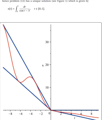
In fact, we can explicitly solve problem (12) because the differential equation and the initial condition yield
x(t) = 1
cost−3 for allt∈[0,L], andx(0) = 0,
hence problem (12) has a unique solution (see Figure 1) which is given by
x(t) = t
0 dr
cosr−3, t∈[0,L].
3 Construction of lower and upper solutions
In general, condition (H1) is the most difficult to check among all the hypotheses in Theorem 1. Because of this, we include in this section some sufficient conditions on the existence of linear lower and upper solutions for problem (1) in particular cases We begin by considering a problem of the form
x(t) =f(x(τ(t,x))) for a.a.t∈I0= [t0,t0+L],
x(t) =k(t) for allt∈I−= [t0−r,t0], (13)
where f ∈C(R) and k∈C(I−).
Proposition 1 Assume that f is a continuous function satisfying
lim
y→+∞f(y) = +∞; (14)
lim
y→−∞f(y) =−∞; (15)
lim y→±∞
f(y)
y <
1
L. (16)
Then there exist m,m¯ >0such that the functions
α(t) =
ϕ∗, if t<t0,
m(t0−t) +ϕ∗,if t≥t0, (17)
and
β(t) =
ϕ∗, if t<t0, ¯
m(t−t0) +ϕ∗,if t≥t0, (18)
are, respectively, a lower and an upper solution for problem (13), where
ϕ∗= mint∈I
− k(t), ϕ
∗= max
t∈I− k(t).
In particular, problem (13) has maximal and minimal solutions between aand b, and this does not depend on the choice ofτ.
Proof. Conditions (15) and (16) imply that
lim y→−∞
y−ϕ∗ f(y) >L,
so there existsy1< min{0,t} such that
0>f(y)> y−ϕ∗
L ify≤y1. (19)
On the other hand, condition (14) implies that there existsy2> 0 such that
f(y)>0 ify≥y2. (20)
Let l= min{f(y):y1≤y ≤y2}. By condition (15) and continuity off, there existsy3≤
y1such that
and this choice ofy3also provides that
f(y3)≤f(y) for ally≥y3, (22)
and, by virtue of (19),
f(y3)> y3−ϕ∗
L . (23)
Now, define a as in (17), with m=ϕ∗−y3
L . Notice that a(t) ≤ k(t) for all t Î I-,
α(t) = y3−ϕ∗
L for all tÎ I0 and
min
t∈I α(t) =α(t0+L) =−mL+ϕ∗=y3,
so we deduce from (22) and (23) that for alltÎI0we have
α(t) =−m<f(y
3) = min
y≥minIα(t)
f(y). (24)
In the same way, we can find ¯y3≥max{0,ϕ∗} such thatb defined as in (18) with ¯
m= ϕ∗−¯y3
L satisfies that b(t)≥k(t) for alltÎ I-and
β(t) =m¯ ≥ max
y≤maxIβ(t)
f(y) for allt∈I0. (25)
So we deduce from (24) and (25) that aand bare lower and upper solutions for pro-blem (13).
Example 4The function
f(y) =
sgn (y) logy, ify∈(−∞,−1)∪(1,∞), sin(πy), ify∈[−1, 1],
satisfies all the conditions in Proposition 1 for every compact interval I0. So the cor-responding problem (13) has at least one solution for any choice of k∈C(I−) and
τ ∈C(I,I).
We use now the ideas of Proposition 1 to construct lower and upper solutions for the general problem (1).
Proposition 2 Let k∈C(I0)and let f : I0 × ℝ2 ® ℝbe a Carathéodory function.
Assume that there exist Fα,Fβ ∈C(R)such that for a.a. tÎ I0 and all yÎ ℝwe have
f(t,x,y)≥Fα(y)for all x≤ϕ∗ (26)
and
f(t,x,y)≥Fβ(y)for all x≤ϕ∗ (27)
Moreover, assume that the next conditions involving Faand Fbhold:
lim
y→−∞Fα(y) =−∞, (28)
lim y→−∞
Fα(y)
y <
1
L, (30)
lim
y→+∞Fβ(y) = +∞, (31)
Fβis bounded from above in (−∞, 0], (32)
lim y→+∞
Fβ(y)
y <
1
L. (33)
Then there exist m,m¯ ≥0such thata and bdefined as in (17), (18) are lower and upper solutions for problem (1) withΛ= 0,and this does not depend on the choice ofτ.
Proof. Reasoning in the same way as in the proof of Proposition 1, we obtain that there existsm≥0 such thata(t)≤*for alltÎ I-and
α(t) =−m≤ min y≥minIα
Fα(y) for a.a.t∈I0.
Asa(t)≤*for alltÎI, we obtain by virtue of (26) that
α(t)≤ min
y≥minIα
f(t,α(t),y) for a.a.t∈I0.
In the same way there exists m¯ ≥0 such thatb(t)≥* for alltÎ I-and
β(t) =m¯ ≥ min
y≥maxIβ
f(t,β(t),y) for a.a.t∈I0.
Therefore, aandbare lower and upper solutions for problem (1).
Example 5Let Fbe the function defined in Example 4 and consider the problem
x(t) =−(x+π)|x+π|γg(t,x) +F(x(τ(t,x))) for a.a.t∈[0,L],
x(t) =−tcostfor allt∈[−π, 0], (34)
whereg≥0,L> 0, andgis a nonnegative Carathéodory function.
In this case, we have*= -π, * ≈0.5611, and the functionf(t,x,y) which defines the equation satisfies
f(t,x,y)≥F(y) ifx≤ −π andf(t,x,y)≤F(y) ifx≥ −π,
so in particular conditions (26) and (27) hold. As conditions (28)-(33) also hold (see Example 4) we obtain that there exist m,m¯ >0 such thata andbdefined as in (17), (18) are lower and upper solutions for problem (34) for any choice of τ. In particular, if there existsψÎL1(I0) such that for a.a.tÎI0and allxÎ [a(t),b(t)] we haveg(t,x)
≤ψ(t), then problem (34) has maximal and minimal solutions betweenaandb.
Remark 3 Notice that the lower and upper solutions obtained both in Propositions 1 and 2 satisfy a slightly stronger condition than the one required in Definition 1.
Acknowledgements
Authors’contributions
Both authors’contributions to this paper are similar and it is impossible to say which part corresponds to each author’s work. All authors read and approved the final manuscript.
Competing interests
The authors declare that they have no competing interests.
Received: 13 May 2011 Accepted: 20 January 2012 Published: 20 January 2012
References
1. Figueroa, R, Pouso, RL: Minimal and maximal solutions to second-order boundary value problems with state-dependent deviating arguments Bull. Lond Math Soc.43, 164–174 (2011). doi:10.1112/blms/bdq091
2. Arino, O, Hadeler, KP, Hbid, ML: Existence of periodic solutions for delay differential equations with state dependent delay. J Diff Equ.144(2), 263–301 (1998). doi:10.1006/jdeq.1997.3378
3. Dyki, A: Boundary value problems for differential equations with deviated arguments which depend on the unknown solution. Appl Math Comput.215(5), 1895–1899 (2009). doi:10.1016/j.amc.2009.07.042
4. Dyki, A, Jankowski, T: Boundary value problems for ordinary differential equations with deviated arguments. J Optim Theory Appl.135(2), 257–269 (2007). doi:10.1007/s10957-007-9248-3
5. Jankowski, T: Existence of solutions of boundary value problems for differential equations in which deviated arguments depend on the unknown solution. Comput Math Appl.54(3), 357–363 (2007). doi:10.1016/j.camwa.2007.01.022 6. Jankowski, T: Monotone method to Volterra and Fredholm integral equa-tions with deviating arguments. Integ
Transforms Spec Funct.19(1-2), 95–104 (2008)
7. Walther, HO: A periodic solution of a differential equation with state-dependent delay. J Diff Equ.244(8), 1910–1945 (2008). doi:10.1016/j.jde.2008.02.001
8. Hartung, F, Krisztin, T, Walther, HO, Wu, J: Functional differential equations with state-dependent delays: theory and applications. Hand-book of Differential Equations: Ordinary Differential Equations, vol. III. pp. 435– 545.Elsevier/North-Holland, Amsterdam (2006)
9. Cid, JÁ: On extremal fixed points in Schauder’s theorem with applications to differential equations. Bull Belg Math Soc Simon Stevin.11(1), 15–20 (2004)
doi:10.1186/1687-2770-2012-7
Cite this article as:Figueroa and Pouso:Minimal and maximal solutions to first-order differential equations with state-dependent deviated arguments.Boundary Value Problems20122012:7.
Submit your manuscript to a
journal and benefi t from:
7Convenient online submission
7 Rigorous peer review
7Immediate publication on acceptance
7 Open access: articles freely available online
7High visibility within the fi eld
7 Retaining the copyright to your article