Square and Cube Difference Labeling of Cycle Cactus, Special Tree and a New Key Graphs

Vol. 8, No. 2, 2014, 115-121

ISSN: 2279-087X (P), 2279-0888(online) Published on 17 December 2014

www.researchmathsci.org

115

Annals of

Square and Cube Difference Labeling of Cycle Cactus,

Special Tree and a New Key Graphs

Sharon Philomena. V1 and K. Thirusangu 2

1

P.G.Department of Mathematics, Women’s Christian College Chennai-600006, Tamilnadu, India

2

Department of Mathematics, S.I.V.E.T College, Tamilnadu, India Email: [email protected]

Received 1 October 2014; accepted 21 November 2014

Abstract. Let G be a (p, q) graph. G is said to be a square difference labeling if there exists a injection f : V(G) → {0,1,2,…,n-1} such that the edge set of G has assigned a weight defined by the absolute square difference of its end-vertices, the resulting weights are distinct. A graph which admits square difference labeling is called square difference graph. Shiama has obtained square difference labeling for some graphs like path, cycle, star (K1,n-1), fan, crown (Cn⨀K1). Let G be a (p, q) graph. G is said to be a cube difference

labeling if there exists a injection f: V(G) → {0, 1, 2, …, n-1} such that the edge set of G has assigned a weight defined by the absolute cube difference of its end-vertices, the resulting weights are distinct. A graph which admits cube difference labeling is called cube difference graph. We have proved the square and cube difference labeling for graphs like cycle cactus graph Ck(3) and the tree <K1,n: 2> and a newly defined key graph

in this paper.

Keywords: Square difference labeling, Cube difference labeling, cycle cactus, tree <K1,n:

2> and key graph

AMS Mathematics Subject Classification (2010): 05C78 1. Introduction

A function f is a square difference labeling of a graph G of size n if f is an injection from V(G) to the set {0, 1, 2, … , n-1} such that , when each edge uv of G has assigned the weight│[f(u)]2 - [f(v)]2, the resulting weights are distinct.

116

Definition 1.1. Let G = ( V(G), E(G) ) be a graph .G is said to be square difference labeling if there exist an injection f : V(G) → {0, 1, …., n-1} such that the induced function f * : E(G) → N given by f *(uv) = │[f(u)]2 - [f(v)]2│ is injective.

Definition 1.2. A graph which satisfies the square difference labeling is called the square difference graph.

Definition 1.3. Let G = ( V(G), E(G) ) be a graph .G is said to be cube difference labeling if there exist an injection f : V(G) → {0, 1, …., n-1} such that the induced function f * : E(G) → N given by f *(uv) = │[f(u)]3 - [f(v)]3│ is injective.

Definition 1.4. A graph which satisfies the cube difference labeling is called the cube difference graph.

Definition 1.5. A cactus is a connected graph in which any two simple cycles have at most one vertex in common Ck(n) (n copies of cycles Ck).

Definition 1.6. A <K1,n: 2> is a tree of diameter 4 obtained from the n bistar Bn,n by sub

dividing the middle edge with a new vertex.

Definition 1.7. A key graph is a graph obtained from K2 by appending one vertex of C5 to

one end point and Hoffman tree PnΘ K1 to the other end point of K2

2. Main result

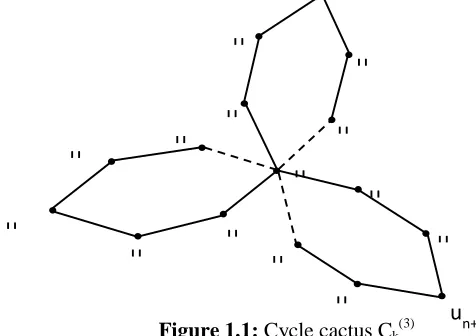
Theorem 2.1. The cycle cactus graph Ck(3) admits cube difference labeling k ≥ 3.

Proof: Let Ck (3)

be a cycle cactus graph, k ≥ 3. Where k is the number of vertices in cycle Ck of cycle cactus graph Ck(3). Denote the vertices of the cycle Ck in the cycle cactus

graph Ck (3)

as u1, u2, …, un in the clockwise direction. Denote the vertices of first copy of

cycle Ck as un+1, …, un+m in the clockwise direction. Similarly denote the vertices of

second copy of cycle Ck as un+m+1, …, un+m+p in the clockwise direction. Note that

│V(G)│= 3n-2 and│ E(G) │= 3n.

Figure 1.1: Cycle cactus Ck(3)

u u

1 u 2

u 3

u

u n

u n+1

u n+2

u n+ u

n+4 u

n+ u

n+m+ u

n+m+2 u

n+m+3 u

n+m+4 u

New Key Graphs

117 The vertex labeling for the graph Ck

(3)

is defined as follows.

f (u) = 0, f (ui) = i , 1 ≤ i ≤ n (1.1)

Now the edge labels are obtained as follows.

f is called cube difference labeling if f*(uv) = │[f(u)]3 - [f(v)] 3│for every uv ∈ E(G) are all distinct where u, v ≥ 0.

Let the edge sets be

E1 = {uui / 0 ≤ i ≤ n} and

E2 = {uiui+1 / 1 ≤ i ≤ n} (1.2)

Let the edge labels be

f *(uui) = i 3

, 1 ≤ i ≤ n and

f *(uiui+1) = 3i2 + 3i + 1 , 1 ≤ i ≤ n (1.3)

Hence the edges are distinct. Hence the cycle cactus graph Ck (3)

admits a cube difference labeling.

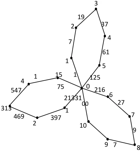
An illustration of the above theorem is shown in Figure 1.2

Figure 1.2: Cube difference labeling of cycle cactus C6 (3)

Theorem 2.2. The <K1,n: 2> admits cube difference labeling.

Proof: Let <K1,n: 2> be a tree. Denote the vertices which are adjacent to u1 as u2, …, un in

the anticlockwise direction. Denote the vertices which are adjacent to the vertex un+1 as

un+2, un+3, …,un+m in the clockwise direction. Let u1, u0, un+1be the path. Note that

│V(G)│= 2n + 3 and│ E(G) │= 2n + 2. 0 1

2

3

4

5

6

7

8 9

10 1

2 313

4 15 1

19

7

37

61

125

216

00 27

9

7 21331

75

397 469

118

Figure 2.1. Tree K<1,n: 2>

The vertex labeling for the tree <K1,n: 2> is defined as follows.

f(u) = 0,

f(ui) = i, 1 ≤ i ≤ n (2.1)

From the above definition in (2.1) it is obvious that the vertex labels are distinct. Now the edge labels are obtained as follows.

f is called cube difference labeling if f *(uv) = │[f(u)]3 –[f(v)]3│for every uv ∈ E(G) are all distinct where u, v ≥ 0.

Let the edge sets be

E1 = {uui / 1 ≤ i ≤ n}

E2 = {uiuj / 1 ≤ i ≤ n , 2 ≤ j ≤ n+m} (2.2)

Let the edge labels be

f *(uui) = i3 , 1 ≤ i ≤ n

f *(uiuj) = i3 – j3 , 1 ≤ i ≤ n , 2 ≤ j ≤ n+m (2.3)

Hence the edges are distinct. Hence the tree <K1,n: 2> admits cube difference labeling.

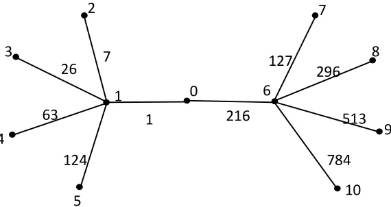
An illustration of the above theorem as follows.

Figure 2.2: Cube difference labeling of <K1,4: 2>

0 1

2

3

4

5

6

7

8

9

10

1 216

7 26

63

124

127

296

513

784 u

5

u 0 u

1 u

2 u

3

u 4

u

6 u_n

u n+1

u n+2

u n+3

u n+4

u n+5

u n+m

New Key Graphs

119

Figure 2.3: Cube difference labeling of <K1,6: 2>

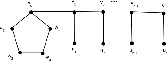
Theorem 2.3. The key graph C5⨀Pn admits a square difference labeling.

Proof: Let the graph G be a key graph C5⨀Pn. The vertex set of G is { w1, w2,……….. w4,

v0, v1,v2,……….vn, u1,u2,……….un} where wi , 1 ≤ i ≤ 4, ui, vi 0 ≤ i ≤ n. Clearly G has

2n+5 vertices and 2n+5 edges.

Figure 2.4: Key graph C5⨀Pn

Let │V(G)│= 2n+5 and │E(G)│= 2n+5.

The mapping f : V(G) → {0,1,2,…,n-1} is defined by f(u) = 0, f(ui) = i,

1 ≤ i ≤ n and the induced function f * : E(G) → N is defined by (i) f * (uui) = │[f(u)]2 – [f(ui)]2│ = i2, 1 ≤ i ≤ n.

(ii) f * (uiui+1) =│[f(ui)] 2

–[f(ui+1)] 2_│

= 2i + 1, 1 ≤ i ≤ n. (iii)f * (uiui+2) = │[f(ui)]

2

– [f(ui+2)] 2

│ = 4i + 4, 1 ≤ i ≤ n.

Here the edge sets are (i) E1= {uui/ 0 ≤ i ≤ n}

(ii) E2= {uiui+1 / 1 ≤ i ≤ n}

(iii) E3 = {uiui+2/ 1 ≤ i ≤ n}

5

0 1

2 3

4

6 ₇

9

10

111

121

1 141

8

1 ₅₁₂

217104881

81916

121621

1685271 223

34233 7 26

63

12463

215

…

w

1

v

0

w

2 w₃

w

4

v

1 v2

u_{1 u}

2

v

n-1

u

n-1

v

n

u

120

Here the edges are distinct. Hence the key graph C5⨀Pn admits a square difference

labeling.

Theorem 2.4. The key graph kn( C5 ⨀ Pn )admits cube difference labeling.

Proof: Denote the key graph C5⨀ Pn as G. The vertex set of G is { w1, w2,... w4, v0,

v1,v2,……….vn, u1,u2,……….un} where wi , 1 ≤ i ≤ 4, ui, vi 0 ≤ i ≤ n. Clearly G has 2n+5

vertices and 2n+5 edges.

Define f : V(G) → {0,1,2,…..,2n+4} as follows,

f(u1) = 0, f(ui) = i, 2 ≤ i ≤ n , f(vi) = i, 1 ≤ i ≤ n, f(wi) = i, 1 ≤ i ≤ 5,

and the induced function f* : E (G) → N is defined by (i) f*(uui) = |[f(u)]3 – [f(ui)]3|= i3 , 1 ≤ i ≤ 2n.

(ii) f*(uiui+1) = |[f(ui)] 3

– [f(ui+1)] 3

|= 3i2+3i+1, 1≤ i ≤ 2n. (iii) f*(uiui+2) = |[f(ui)]3 – [f(ui+2)]3|= 6i2+12i+8, 1≤ i ≤ 2n.

Here the edge sets is E = { wi wi+1, 0 ≤i ≤ 4} ∪ { v0, w5}∪ { vi vi+1, 1 ≤ i ≤ n-1} ∪

{ ui vi , 1 ≤i ≤ n-1} ∪ { v0 v1}

Here the edges are distinct. Hence the key graph C5⨀Pn admits a cube difference

labeling.

3. Conclusion

In this paper the cycle cactus graphs, tree <K1,n: 2 > and key graph are investigated for

the square and cube difference labeling. This labeling can be verified for some other graphs.

REFERENCES

1. F.Harrary, Graph Theory, Narosa Publishing House, New Delhi, India, 2001.

2. J.A.Gallian, A dynamic survey of graph labeling, Electronics Journal of Combinatorics, 16 (2013) # DS6.

3. K.Das, Some algorithms on cactus graphs, Annals of Pure and Applied Mathematics, 2(2) (2012) 114-128.

4. J.Shiama, Square sum labeling for some middle and total graphs, International Journal of Computer Applications, 37 (2912) 1-8.

5. J.Shiama, Square difference labeling for some path, fan and gear graphs, International Journal of Scientific and Engineering Research, 4 (2013) 1-9.

6. J.Shiama, Some special types of Square difference graphs, International Journal of Mathematical Archives, 3 (2012) 2369-2374.

7. J.Shiama, Square difference labeling for some graphs, International Journal of Computer Applications, 44 (2012) 30-33.

New Key Graphs

121

9. S.K.Vaidya and N.B.Vyas, Antimagic labeling of some path and cycle related graphs, Annals of Pure and Applied Mathematics, 3(2) (2013) 119-128.

10. N.Khan, Cordial labelling of cycles, Annals of Pure and Applied Mathematics, 1(2) (2012) 117-130.

11.N.Khan, A.Pal and M.Pal, Edge colouring of cactus graphs, Advanced

Modeling and Optimization, 11(4) (2009) 407-421.

12. N.Khan, M.Pal and A.Pal, L(0,1)-labelling of cactus graphs, Communications and Network, 4 (2012) 18-29.

13. N.Khan and M.Pal, Cordial labelling of cactus graphs, Advanced Modeling and Optimization, 15 (2013) 85-101.

14. N.Khan and M.Pal, Adjacent vertex distinguishing edge colouring of cactus graphs, Inter. J. Engineering and Innovative Technology, 4(3) (2013) 62-71.

15. N.Khan, M.Pal and A.Pal, (2,1)-total labelling of cactus graphs, Journal of Information and Computing Science, 5(4) (2010) 243-260.