Single-Label Multi-Class Image Classification by Deep Logistic Regression

The Thirty-Third AAAI Conference on Artificial Intelligence (AAAI-19)

Single-Label Multi-Class Image Classification by Deep Logistic Regression

Qi Dong,

1

_{Xiatian Zhu,}

2

_{Shaogang Gong}

1

1_{Queen Mary University of London,}2_{Vision Semantics Ltd.}

[email protected], [email protected], [email protected]

Abstract

The objective learning formulation is essential for the success of convolutional neural networks. In this work, we analyse thoroughly the standard learning objective functions for multi-class multi-classification CNNs: softmax regression (SR) for single-labelscenario and logistic regression (LR) for multi-label scenario. Our analyses lead to an inspiration of exploiting LR for single-label classification learning, and then the disclosing of thenegative class distractionproblem in LR. To address this problem, we develop two novel LR based objective functions that not only generalise the conventional LR but importantly turn out to be competitive alternatives to SR in single label classification. Extensive comparative evaluations demonstrate the model learning advantages of the proposed LR functions over the commonly adopted SR in single-label coarse-grained object categorisation and cross-class fine-grained person in-stance identification tasks. We also show the performance superiority of our method on clothing attribute classification in comparison to the vanilla LR function.The code had been made publicly available.

Introduction

Convolutional neural networks (CNNs) (LeCun et al. 1989) have demonstrated impressive performance success in a wide variety of image recognition problems (Krizhevsky, Sutskever, and Hinton 2012; He et al. 2016; Liu et al. 2016). Two common problems aresingle-label(one class label per image) andmulti-label(multiple class labels per image) clas-sification. Whilst both problems have the same learning objective of inducing a multi-class classifier CNN model through supervised training, their standard objective learning functions arerather different.

Specifically, in single-label classification learning, we of-ten adopt thesoftmax regression(SR) learning algo-rithm. This is based on the per-sample single-label and class-exclusion assumptions (Bridle 1990). For multi-label classifi-cation in which a data sample may be tied with multiple class labels, we instead adopt the logistic regression (LR) learning algorithm (Bishop 2006). Without the “single-label” and “class-exclusion” prior, LR considers per-sample prediction of all individual class labelsindependently.

Copyright c2019, Association for the Advancement of Artificial Intelligence (www.aaai.org). All rights reserved.

It is intuitive that single-label classification is a special case of multi-label classification. Hence, LR should be appli-cable for single-label classification. Surprisingly, despite that both SR and LR have been extensively studied and exploited for learning single-label and multi-label classification inde-pendently, their comparison in deep learning of single-label classification has never been investigated systematically in the literature to our knowledge. A few fundamental questions remain unclear: How advantageous is thede facto standard

choice SR over LR for single-label classification on earth? Is LR possibly competitive with or even superior to SR?

In this work, we investigate the potential and validity of

the Logistic Regression learning algorithm for single-label multi-class classificationin theory and practice. We observe that although SR has an advantage of conducting class dis-criminative learning via posing a competition mechanism be-tween the ground-truth and other classes per training sample, it may simultaneously distort the underlying data manifold geometry which may in turn hurt the model generalisation capability (Belkin, Niyogi, and Sindhwani 2006). This is because in SR all non-ground-truth classes are identically pushed away from the labelled ground-truth class in a homo-geneous fashion with the class-to-class correlation ignored in model learning. On the contrary, LR avoids this limitation due to that each class is modelled independently as a separate binary classification task (Bishop 2006). This allows the in-trinsic inter-class geometrical correlation to emerge naturally in a data-mining manner.

In light of the above theoretical merit, we particularly study the efficacy of LR for single-label classification learning. Em-pirically, we found that the vanilla LR indeed yields less discriminative and generalisable models on image classifica-tion tasks in most cases. With in-depth LR loss and gradient analysis, we identify that thenegative class distraction prob-lem turns out to be the major model learning barrier.

classification based image recognition tasks, coarse-grained object categorisation and fine-grained zero-shot person in-stance identification, by usingfivestandard benchmarks. The results show that our methods perform on par with or out-perform the standard algorithm SR. We further validate the effectiveness of our method in clothing attribute classification with extremely sparse labels per data sample.

Related Work

With the recent surge of interest in neural networks like CNNs, image classification by deep learning has gained mas-sive attention and remarkable success (Krizhevsky, Sutskever, and Hinton 2012; Girshick 2015; Dong, Gong, and Zhu 2017b; Liu et al. 2016; Lin et al. 2017; Dong, Gong, and Zhu 2017a). We have witnessed significant advances in many aspects including network architecture improvement (He et al. 2016), nonlinear activations (Maas, Hannun, and Ng ), layer designs (Lin, Chen, and Yan 2014), regularisation techniques (Srivastava et al. 2014), optimisation algorithms (Kingma and Ba 2015), and data augmentation (Krizhevsky, Sutskever, and Hinton 2012).

Essentially, these existing methods are mostly used and grounded on the well-established learning algorithms such as softmax regression (SR) (Luce 2005; Bridle 1990) and logistic regression (LR) (Little 1974; Mor-Yosef et al. 1990). Impacted by the traditional design principles (Goodfellow, Bengio, and Courville 2016; Krishnapuram et al. 2005), LR is often used to produce the prediction output of multi-label multi-class classification models (Liu et al. 2016; Chua et al. 2009), whilst SR to that of single-label multi-class clas-sification models (Krizhevsky, Sutskever, and Hinton 2012; Russakovsky et al. 2015) in current deep learning practice.

Although takingdifferentlearning formulations, both SR and LR algorithms aim to train a multi-class neural network classifier which, once trained, is able to predict the top one or multiple class label(s) of new samples at test time. One reason for this design discrepancy is that in SR, the single-label constraint facilitates the learning of a multi-class classifier. Although lacking the single-label class prior, LR has a merit of individually learning per-class distributions and better maintaining the class manifold structures (Bishop 2006). In spite of that, LR is howeverrarelychosen to learn single-label multi-class classification by existing methods, leaving its potential efficacy for image recognition remaining unknown in deep learning. To fill this gap, we systematically study this ignored problem, identify and address a negative class distraction (NCD) problem.

The NCD problem is concerned with imbalance learning with a particular focus on positive and negative classes per training sample. It is therefore related to the conventional class imbalanced learning problem (Japkowicz and Stephen 2002; Weiss 2004; He and Garcia 2009; Dong, Gong, and Zhu 2018; Huang et al. 2016). Whilst sharing some theoretical concept in general, the NCD problem in our context is funda-mentally different because it isindependentof thetraining data distributionwhich however is the core problem existing class imbalanced learning methods aim to address. Differ-ently, the NCD problem is underpinned in thetarget class

space, occurring in the multi-class joint optimisation process

on each training sample. A larger class space leads to a more serious NCD problem. In other words, the NCD problem remains even withabsolutely balanced(equally sized) train-ing samples per class. Besides, LR bias correction has been extensively studied (King and Zeng 2001; Schaefer 1983; Qiu et al. 2013; Heinze and Schemper 2002) but still focus-ing on the data imbalance issue, rather than the NCD problem as considered in this work.

Delve Deep into Deep Learning Classification

Supervised deep learning algorithms learn to classify in-put images into target class labels, given a training set of nimage-label pairsD = {(xi, yi)}ni=1 whereyi ⊆ Y = {1,2,_{· · ·}, K_}specifies the ground-truth label set of image

xiwith one (single-label) or multiple (multi-label) class(es) associated. There are totallyKpossible classes. Supervised learning of such multi-class classifiers is generally conducted based on estimating probabilistic class distributions p of

training images with the elementpk =p(k|x),k∈ Y. Probability Distribution Estimation. To makepk repre-sent valid probability values, one common approach to nor-malising individualpk is to apply the logistic (or sigmoid) function (Little 1974; Mor-Yosef et al. 1990) to squash the raw outputz=φ(x|θ)into the interval(0,1)as:

pk =p(k|x;θ) =σ(z)k = 1 1 +e−zk

= e zk

ezk+ 1, k∈ Y={1,2,· · ·, K}

(1)

whereθdenotes the model parameters that project an input xinto a logit spacezvia a to-be-learned mappingφ.

In essence, Eq (1) models a Bernoulli distribution for each individual class (a binary-value random variable) indepen-dently, i.e. the model learns to predict the positive probability p(1 _|x) for each class k. Therefore, it naturally fits the

multi-labelclassification scenario: Each image sample can be associated with multiple (an unknown number) class la-bels in any possible combinatorial ways. Eq (1) is known as Logistic Regression(LR).

Single-labelclassification is another common scenario in which only one class label is outputted for a single sam-ple. This implicitly assumes a mutual exclusion relation-ship between all classes. Hence, we can further require theentirevectorpas a multi-class probability distribution:

PK

k=1pk= 1andpk≥0. To that end, the softmax function is often employed (Luce 2005; Peterson and S¨oderberg 1989; Bridle 1990). Formally, we exponentiate and normalise the logitzto obtain a valid probability vectorpas:

pk =p(k|x;θ) =h(z)k = e zk PK

j=1ezj ,

with k∈ Y={1,2,· · · , K}

(2)

Eq (2) models a categorical distribution of a discrete variable over multi-classescollectivelyandinter-dependently. Eq (2) is calledSoftmax Regression(SR).

-40 -30 -20 -10 0 10 20 30 40 -30

-20 -10 0 10 20 30 40

(c) SS-LR

-40 -30 -20 -10 0 10 20 30 40 -40

-30 -20 -10 0 10 20 30

(b) LR

-30 -20 -10 0 10 20 30

-40 -30 -20 -10 0 10 20 30 40

(a) SR

-30 -20 -10 0 10 20 30

-40 -30 -20 -10 0 10 20 30 40

1 2 5 6 8

-30 -20 -10 0 10 20 30

-40 -30 -20 -10 0 10 20 30 40

1 2 5 6 8

-30 -20 -10 0 10 20 30

-40 -30 -20 -10 0 10 20 30 40

1 2 5 6 8

-30 -20 -10 0 10 20 30

-40 -30 -20 -10 0 10 20 30 40

1 2 5 6 8 Bee Bed Apple

Bicycle

-30 -20 -10 0 10 20 30

-40 -30 -20 -10 0 10 20 30 40

1 2 5 6 8

Baby

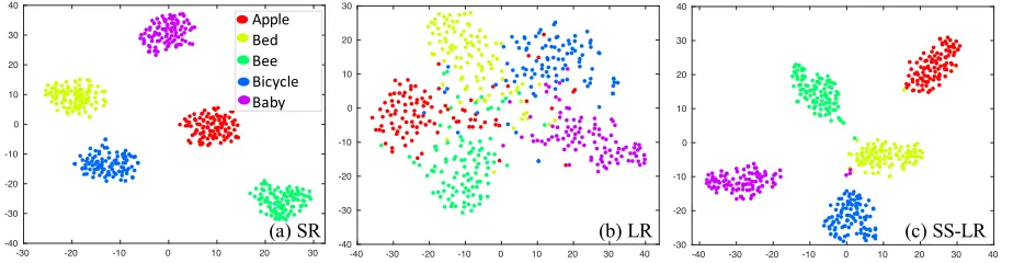
Figure 1: Colour-coded t-SNE feature embedding of 5 CIFAR100 object classes produced by (a) SR, (b) LR, and (c) the proposed SS-LR (Eq (6)) loss functions. It is evident that in the feature embedding space by the vanilla LR, different classes are poorly distinguishable with severe cross-class boundary overlap. In contrast, our SS-LR yields more discriminative feature embedding by addressing the NCD problem involved in model optimisation. Best viewed in colour.

with the data empirical distribution by a cross-entropy mea-surement (Goodfellow, Bengio, and Courville 2016). The specific learning objective function relies on the regression form of the model’ s prediction.

In case of multi-label classification, the objective function for maximum likelihood learning is formulated as:

LLR(x, y) =−

K X

k=1

qklog(pk)+(1−qk) log(1−pk)

(3)

This objective function aggregates the negative log-likelihood of all class-wise Bernoulli distributions.

In case of single-label classification, we directly use the cross-entropy between the ground-truth class distributionq

of the training datum and the predicted class distributionp

of the model to form the objective function.q=δk,yis Dirac delta which equals to 1 ifk=y, and 0 otherwise. The learning

objective function is written as:

LSR(x, y) =−

K X

k=1

qklogpk=−logpy (4)

Remarks. In essence, the key of model learning is to induce the target multi-class feature embedding space. A general-isablefeature space should be characterised by an accurate inter-class manifold structure. Given a training samplex, SR

enforces acompetitionbetween the ground-truth and other classes to learn the model discrimination capability: the soft-max output always sums to 1, subject to that an increase in the estimation of one class necessarily corresponds to a decrease in the estimation of others. Whilst this competition significantly helps learn discriminative inter-class boundaries, it may distort the underlying inter-class manifold structure therefore potentially hurting the model generalisation capabil-ity (Belkin, Niyogi, and Sindhwani 2006), since SR treats all non-ground-truth classesidenticallyby pushing them away from the ground-truth class in a homogeneous manner. In contrast, LR learns to induce the inter-class manifold struc-ture from the training data, enabling a natural emergence of the underlying multi-class manifold geometry.

Focus Rectified Logistic Regression

The Negative Class Distraction Problem

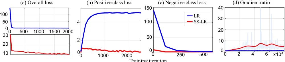
Despite the theoretical merit of LR, directly using the vanilla LR often leads to inferior model performance than SR, as shown in Fig 1 (b). Why does this happen? To examine this problem in LR, we track and analyse the training loss and gradient quantities (the blue curves in Fig 2). We observe that at the beginning of model training, the LR loss drops dramatically until near 0 (see Fig 2 (a)). Further decomposing the LR loss into two parts: the positive class loss on the ground truth class (see Fig 2(b)) and negative class loss on all non-ground-truth classes (see Fig 2(c)), we find that at early training iterations, (1) the starting negative class loss is far larger than the starting positive class loss (e.g. 140 vs 0.4); and (2) the positive class loss increasesunexpectedly, while the negative class loss drops fast. This suggests that at the early training stage, the overall LR loss is dominated by negative classes therefore the positive class is largely ignored. We call this effect asnegative class distraction(NCD).

The NCD problem is intrinsic to single-label multi-class classification. Specifically, suppose aK-class setting, each training samplexhas only one positive class (the ground-truth labely) but(K₋1)negative classes. With the vanilla

LR learning objective (Eq (3)), the positive class obtains insufficient attention, especially whenKis large. Therefore, the training is hinted by the severe learning bias towards the negative classes. Such a biased loss composition deceives the model to converge towards some poor local minima with the negative classes well satisfied (Fig 2(c)) whilst the positive class largely ignored (Fig 2(b)). This can be further justified by the nearly zero gradient ratio of positive to negative classes (Fig 2)(d)). The NCD problem similarly exists in multi-label classification with sparse labels per sample (Fig 4).

Often, the inherent learning difficulty and velocity of dif-ferent classes can be distinct, as indicated in the accuracy variety over object classes (Deng et al. 2009). Hence, treating all negative classes per sample identically as Eq (3) may be

nega-(b) Positive class loss (c) Negative class loss

0 2 4 6 8

Training iterations ₁₀4

0 10 20 30 40

Gradient ratio ₀

20 30 40

0 2 6 x104

10

4

500 1000 1500 2000

0 50 100

500 1000 1500

500 1000 1500 2000

10 20 30

0 2000

0 50 100

10 20 30

(a) Overall loss (d) Gradient ratio

0

500

Training iteration

0

50

100

150

Negative classes loss

100

0 50

250

0 500

LR SS-LR

150

0

1000

2000

Training iteration

2

4

Negative classes loss

0 1000 2000

2 4

0

Training iteration

Figure 2: Negative class distraction effect of LR on Tiny ImageNet. . (a) Overall training loss values; The loss of (b) the positive class and (c) the negative classes; (d) Gradient ratio of positive to negative classes.

tive class selection mechanisms to rectify the biased learning focus of the vanilla LR in a hard mining principle: A training samplexis more (less) informative to hard (easy) classes.

Rectification by Negative Class Hard Selection

We confine the learning focus to non-trivial (hard) other than all negative classes. Specifically, we use the predicted proba-bilitypkas the hardness measurement to rank(K−1) nega-tive classes in the descending order. We then choose the top negative classes to formulate the objective loss function as:

LhsLR(x, y) =−log(py)−α X

k∈fhs(m|p,y)

log(1−pk)

(5)

where the hard selection functionfhs(m|p, y)returns the top m%negative classes with highest prediction probabilities.

We add a balancing weightαto trade-off positive and nega-tive classes, inspired by the cost-sensinega-tive learning (Akbani, Kwek, and Japkowicz 2004; He and Garcia 2009).

Adjustingm ∈[0,100]allows us to modulate the focus

rectification degree: with a training sample, we learn the decision boundaries ofm%most confusing negative classes

along with the positive class. We empirically found thatm= 25is satisfactory. Whenm= 100, we attend all negative

classes with a cost-sensitive trade-off between the positive and all negative classes. The weightαcan be intuitively set as inversely proportional to the selected negative class number: α=_bm%(β_K−1)c <1whereβis a hyper-parameter (β= 10in

our experiments). We call thisnegative class Hard Selection

based LR formulation asHS-LR.

Rectification by Negative Class Soft Selection

An alternative to HS-LR is a soft selection of negative classes. Formally, we employ a hardness (probability) adaptive weight

(pk)rto each negative class as:

LssLR(x) =−log(py)−α K X

k=1,k6=y

(pk)rlog(1−pk)

(6)

where r _≥ 0 is the attending parameter that controls the rate of attending hard negative classes and disregarding easy negative classes. Note that whenr= 0, it is equivalent to HS atm= 100. Growingrmakes the focus modulating effect

like-wisely increase. In our experiments, we found thatris not sensitive in a reasonable range of andr= 2is selected

in our main experiments (Fig 7). We setα=_Kβ₋₁since all negative classes are considered.

Our soft selection mechanism achieves the effect of hard class mining in this manner: If a negative classkis a hard class w.r.t.xand receives a higher probabilitypk, its weight (pk)ris larger and hence more attention is assigned. When the value ofpkis small which suggests an easy negative class, the learning attention will be close to 0 and the quantity of classkis significantly down-weighted. We call thisnegative

class Soft Selectionbased LR formulation asSS-LR. The soft selection principle has been used in other meth-ods, e.g. Entropy-SGD (Chaudhari et al. 2016) and focal loss (Lin et al. 2017). Entropy-SGD tackles a different problem of seeking better local minima. The focal loss is more similar to our SS-LR (Eq (6)) but differs in a number of fundamental aspects: (1) Focal loss solves theglobaltraining data sample imbalance whilst SS-LR deals with thelocalsample-wise negative class distraction, independent of the training data distribution over classes. (2) Focal loss is built on the soft-max regression, whilst SS-LR is formulated based on the logistic regression. (3) Focal loss aims to suppress easy train-ing instances in thesamplespace whilst SS-LR handles the per-sample negative classes in theclassspace.

(c) Deepfashion

(a) CIFAR (c) Tiny Imagenet

2.3.Pre-Processing and Data Augmentation

Prior to training, the training, validation, and test data were zero centered by subtracting the mean image from the training data – this pre-processing step, as well as the data loading, was implemented by re-using code given by CS231N instructors during assignments[11].

Given the small size of the training dataset, live data augmentation was applied during training. In particular, images were randomly rotated by up to 60 degrees, zoomed in up to 1.2x magnification, and shifted vertically and horizontally.

In order to perform the data augmentation, Keras’ Image Data Generator implementation was used[6].

3. Methods

To implement my models I am using version r1.2 of Google’s TensorFlow[6] open source deep learning framework, stacked with the included higher level API, Keras[7]. Keras offers a functional API that allows for faster prototyping as well as creation of wide layers such as Inception with significantly less overhead than vanilla TensorFlow.

3.1. Objective Function

As is to be expected, the all the models trained leverage back-propagation to perform gradient updates. The updates were done by minimizing the cross-entropy loss as given by the Softmax function.

[12]. This is of course the standard in the field, but it is worth noting that cross-entropy is preferable to other losses such as the SVM or hinge loss as cross-entropy provides a probabilistic interpretation.

Note that regularization and bias terms were added to each convolutional layer. In particular, L-2 regularization was utilized after early trials showed it outperformed L-1.

3.2. Weight Initialization

The means of initializing all weights for every layer of each model was the Glorot Uniform Initializer, also called the Xavier Uniform Initializer[13], as implemented by Keras. Namely, the weights were drawn from the following distribution, with n being the layer size. [13]

3.3. Optimization Algorithm

Per guideline presented by Justin Johnson in CS231N lecture 7, the primary optimization algorithm used was Adam[14], as implemented by Keras. Early trials tried using stochastic gradient descent, and Adam + Nesterov Momentum[8], all as implemented by Keras, but ultimately, empirical results showed Adam to be superior in my trials.

3.4. Network Regularization

Early on, I experimented with incorporating Dropout [10] with varying rates, and at different points in the network – after each conv layer, before just the input, after pools, and after batch norm layers. However, ultimately I found Batch Normalization [9] to provide much better validation performance for the models that were trained. The idea behind Batch Normalization being that by adding multiple normalizing layers through the network, we can reduce the internal covariate shift from layer to layer within the network.

Of an interesting note, I found that, contrary to common wisdom, utilizing Dropout led to significantly faster training than Batch Normalization, at a cost in validation loss and accuracy – I found Dropout to overfit significantly more than Batch Normalization.

3.5. VGG Style Model Architectures

The VGG Style architecture features a structure (b) SVHN

(a) CIFAR (c) Tiny Imagenet

2.3.Pre-Processing and Data Augmentation

Prior to training, the training, validation, and test data were zero centered by subtracting the mean image from the training data – this pre-processing step, as well as the data loading, was implemented by re-using code given by CS231N instructors during assignments[11].

Given the small size of the training dataset, live data augmentation was applied during training. In particular, images were randomly rotated by up to 60 degrees, zoomed in up to 1.2x magnification, and shifted vertically and horizontally.

In order to perform the data augmentation, Keras’ Image Data Generator implementation was used[6].

3. Methods

To implement my models I am using version r1.2 of Google’s TensorFlow[6] open source deep learning framework, stacked with the included higher level API, Keras[7]. Keras offers a functional API that allows for faster prototyping as well as creation of wide layers such as Inception with significantly less overhead than vanilla TensorFlow.

3.1. Objective Function

As is to be expected, the all the models trained leverage back-propagation to perform gradient updates. The updates were done by minimizing the cross-entropy loss as given by the Softmax function.

[12]. This is of course the standard in the field, but it is worth noting that cross-entropy is preferable to other losses such as the SVM or hinge loss as cross-entropy provides a probabilistic interpretation.

Note that regularization and bias terms were added to each convolutional layer. In particular, L-2 regularization was utilized after early trials showed it outperformed L-1.

3.2. Weight Initialization

The means of initializing all weights for every layer of each model was the Glorot Uniform Initializer, also called the Xavier Uniform Initializer[13], as implemented by Keras. Namely, the weights were drawn from the following distribution, with n being the layer size. [13]

3.3. Optimization Algorithm

Per guideline presented by Justin Johnson in CS231N lecture 7, the primary optimization algorithm used was Adam[14], as implemented by Keras. Early trials tried using stochastic gradient descent, and Adam + Nesterov Momentum[8], all as implemented by Keras, but ultimately, empirical results showed Adam to be superior in my trials.

3.4. Network Regularization

Early on, I experimented with incorporating Dropout [10] with varying rates, and at different points in the network – after each conv layer, before just the input, after pools, and after batch norm layers. However, ultimately I found Batch Normalization [9] to provide much better validation performance for the models that were trained. The idea behind Batch Normalization being that by adding multiple normalizing layers through the network, we can reduce the internal covariate shift from layer to layer within the network.

Of an interesting note, I found that, contrary to common wisdom, utilizing Dropout led to significantly faster training than Batch Normalization, at a cost in validation loss and accuracy – I found Dropout to overfit significantly more than Batch Normalization.

3.5. VGG Style Model Architectures

The VGG Style architecture features a structure (b) SVHN (b) ImageNet

(e) Market1501 (d) DukeMTMC-ReID

(a) CIFAR

Figure 3: Example images of benchmark datasets evaluated.

Experiments

We evaluated the proposed method on (1) single-label ob-ject classification, (2) person instance identification, and (3) multi-label clothing attribute recognition. For each test, we performed 10 independent runs and reported the average re-sult. Note that, outperforming existing best performers by extra complementary techniques is not the focus of our eval-uations. Rather, the key is to investigate the model general-isation performance of the same network model learned by the SR and LR objective functions in a fair test setting.

Single-Label Object Image Classification

Datasets. We used three single-label object classification benchmarks.CIFAR10andCIFAR100(Krizhevsky and Hin-ton 2009) both have 32_×32 sized images from 10 and 100 classes, respectively. We adopted the benchmarking 50,000/10,000 train/test image split on both.Tiny ImageNet (Tiny200)(Deng et al. 2009) contains 110,000 64×64 images from 200 classes. We followed the standard 100,000/10,000 train/val setting. These datasets present varying class num-bers, thus giving a spectrum of different single-label model test scenarios. Example images of these datasets are given in Fig 3.

Experiment setup. We carried out all the following exper-iments in TensorFlow (Abadi et al. 2016). We tested three varying-capacity networks: ResNet-32 (32 layers with 0.7 million parameters) (He et al. 2016), WideResNet-28-10 (28 layers with 36.5 million parameters) (Zagoruyko 2016), and DenseNet-201 (20 million parameters) (Huang et al. 2017). We adopted the top-1 classification accuracy in our evalua-tions. We used the standard SGD with momentum for model training. We set the initial learning rate to 0.1, the momentum to 0.9, the weight decay to10−4_{, the batch size to 128/64/128} for CIFAR/Tiny200/ImageNet, the epoch number to 300. We set the parameter m(Eq (5)) in the range of[25,75] and

r= 2(Eq (6)) (r = 50for ImageNet) by a grid search on the validation dataset. Data augmentation includes horizontal flipping and translation. All models compared used the same training/test data for fair comparative evaluations.

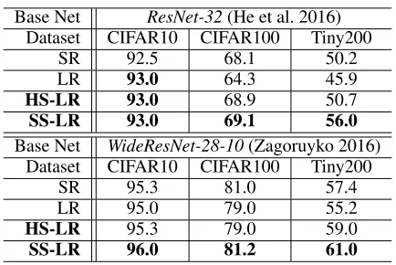
Table 1: Evaluation on single-label object image classifica-tion. Metric: Top-1 accuracy rate (%).

Base Net ResNet-32(He et al. 2016) Dataset CIFAR10 CIFAR100 Tiny200

SR 92.5 68.1 50.2

LR 93.0 64.3 45.9

HS-LR 93.0 68.9 50.7

SS-LR 93.0 69.1 56.0

Base Net WideResNet-28-10(Zagoruyko 2016) Dataset CIFAR10 CIFAR100 Tiny200

SR 95.3 81.0 57.4

LR 95.0 79.0 55.2

HS-LR 95.3 79.0 59.0

SS-LR 96.0 81.2 61.0

Evaluation. Table 1 compares the single-label object cat-egorisation performances between the SR and LR function

variants using the small ResNet-32 and large WideResNet-28-10 architectures. We make these observations:(1)When the class number increases, the vanilla LR suffers a more severe NCD problem and yields much weaker performances than SR. For example, on CIFAR10 with 10 classes, LR per-forms on a par or even slightly better. However, LR is clearly inferior on Tiny ImageNet with 200 classes (On the other hand, this also simultaneously implies a good potential of LR since the results are not far worse).(2)The proposed LR variants notably improve the performance and outperform the SR, especially on tasks with more classes. This indicates that once the NCD problem is properly solved (Fig 2), LR can be a stronger formulation for single-label classification learning. This observation is rarely made in the literature where SR dominants the learning of single-label classifica-tion models.(3)The Soft Selection (SS) strategy consistently yields the best model generalisation, suggesting the advan-tages of exploiting all negative object classes in a hardness adaptive manner.(4)Both small and large nets benefit from the proposed LR algorithms, indicating that our method is generically applicable to different CNN architectures.

Fine-Grained Person Instance Identification

Datasets. We used two popular person instance identifica-tion (a.k.a., person re-identificaidentifica-tion) benchmark datasets in our experiments. TheMarket-1501(Zheng et al. 2015) has 32,668 images of 1,501 different identities (ID) captured from 6 outdoor camera views. We followed the standard 751/750 train/test ID split. TheDukeMTMC(Ristani et al. 2016) consists of 36,411 images of 1,404 IDs from 8 cam-era views. We adopted the benchmarking 702/702 ID split as (Zheng, Zheng, and Yang 2017). Unlike normal image classification, person re-identification (re-id) is a more fine-grained recognition problem of matching person instances across non-overlapping camera views. It is more challenging due to the inherent zero-shot learning knowledge transfer from seen classes (IDs) to unseen classes in deployment, i.e. no overlap between training and test classes.

Experiment setup. We tested two nets, with variant capac-ities, often used in existing re-id methods: ResNet-50 (He et al. 2016) (50 layers with 25.6 million parameters), and MobileNet (Howard et al. 2017) (28 layers with 3.3 million parameters). We adopted two standard performance metrics in thesingle querymode: the Cumulative Matching Charac-teristic accuracy (Rank-1rate) and mean Average Precision

(mAP). We used the Adam optimiser (Kingma and Ba 2015), and set the initial learning rate to 0.0003, the momentum to 0.9, the weight decay to10−4_{, the batch size to 32, and} the maximum epoch number to 300. We trained all methods without using complex tricks in order to focus the evaluation on comparing SR and LR algorithms.

Table 2: Evaluation on person instance identification.

Base Net ResNet-50(He et al. 2016) Dataset Market-1501 DukeMTMC Metric (%) Rank-1 mAP Rank-1 mAP

SR 83.3 65.8 73.7 54.9

LR 81.4 65.0 72.2 54.6

HS-LR 87.1 70.7 77.9 60.1

SS-LR 85.8 69.7 76.7 58.2

Base Net MobileNet(Howard et al. 2017) Dataset Market-1501 DukeMTMC Metric (%) Rank-1 mAP Rank-1 mAP

SR 71.7 50.0 57.0 35.8

LR 51.5 34.3 43.9 27.5

HS-LR 76.4 54.1 63.7 42.5

SS-LR 74.0 53.7 62.9 41.5

algorithms improve the model performance, suggesting that the NCD problem still matters in cross-class recognition.(3) Hard selection (HS) turns out to be the best strategy, as op-posite to object classification (Table 1) where SS is the best performer. This indicates that using every training sample to learn all classes is not necessarily superior, which may nega-tively affect the modelling capacity of mining fine-grained discriminative information among a large number of training classes (751 on Market-1501, and 702 on DukeMTMC).

To validate the statistical significance of our model’s per-formance, we conducted a Wilcoxon signed-rank test on the DukeMTMC results using MobileNet. The test verifies that the improvements in accuracy and mAP rates are statistically significant at the 5% significance level.

Clothing Attributes Recognition

Apart from single-label classification, we evaluated our LR methods on the multi-label classification specially with only a few labels per instance, which also suffers a similar NCD problem. The SR is not applicable in this test.

Dataset. We evaluated a large scale multi-label clothing attribute datasetDeepFashion(Liu et al. 2016). This dataset has 289,222 images labelled with 1,000 fine-grained clothing attributes with a 209,222/40,000/40,000 train/val/test bench-mark setting. Each image is associated withextremelysparse labels, 3 out of 1,000 in average. The training set is also

highly class imbalanced (733:1), therefore presenting a very challenging multi-label classification task. We adopted the standard multi-label classification setting without using aux-iliary types of supervision such as key-points and clothing category as used in (Liu et al. 2016).

Experiment setup. We similarly tested two nets: ResNet-50 (He et al. 2016), and MobileNet (Howard et al. 2017). We adopted two standard performance measurement criteria: mean Average Precision (mAP) and balanced classification accuracy (Dong, Gong, and Zhu 2018; Huang et al. 2016). The latter is particularly designed to remedy the performance evaluation bias towards the majority classes of imbalanced data. For each metric, we evaluated per-image and per-class model performances of top-5 class predictions. We used the

Table 3: Evaluation on multi-label attribute recognition.

Base Net ResNet-50(He et al. 2016) Metric (%) _{Per Img Per Cls}Accuracy _{Per Img Per Cls}mAP

LR 64.8 50.1 21.6 2.5

HS-LR 74.3 59.0 31.5 9.3

SS-LR 73.9 58.7 34.4 9.2

Base Net MobileNet(Howard et al. 2017) Metric (%) _{Per Img Per Cls}Accuracy _{Per Img Per Cls}mAP

LR 62.4 51.9 23.4 4.7

HS-LR 72.2 57.4 28.1 7.2

SS-LR 72.0 55.8 31.0 6.5

Adam optimiser (Kingma and Ba 2015), with the learning rate of 0.0001 for the first 45 epochs and 0.00001 for the last 5 epochs, the weight decay of 0.00004, the momentum of 0.9, and the batch size of 32.

0 1 2 3 4 5

Training iteration 104

0 50 100 150

Training loss

LR SS-LR HS-LR

Training iteration

0 1 2 3 4 5

T

ra

ini

ng l

os

s

0 1 2 3 4 5

Training iteration 104 0

50 100 150

Training loss

LR SS-LR HS-LR

50 100 150

x104

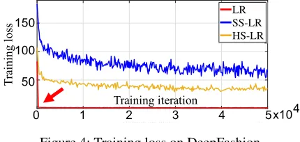
Figure 4: Training loss on DeepFashion.

Evaluation. Table 3 shows the clothing attribute classifica-tion performances of different LR variants. It is observed that: (1)Our LR methods are significantly superior to the vanilla algorithm, which is consistent with the results on single-label object classification and person re-id.(2)Hard and soft selection strategies perform similarly across different nets and metrics. These results suggest the generic advantages of our approach in multi-label classification, confirming the existence of NCD. Moreover, our method also notably out-performs the state-of-the-art result (54.5 per-class accuracy) in the same test setting obtained by (Dong, Gong, and Zhu 2018), further validating the efficacy of our approach.

Figure 4 shows the loss converging process during training. Similar to single label object classification (Fig 2), the vanilla LR is clearly hurt by the NCD problem. In contrast, SS-LR and HS-LR achieve a more stable and healthy model learning process by adaptively hard mining negative classes.

Further Analysis and Discussion

the learning focus of positive classes in training and therefore mitigating the NCD problem.

5 10 15

104 0 0.2 0.4 0.6 SR LR HS-LR SS-LR

0 5 10 15 x104

20 40 60 Training iteration Te st a cc ur ac y (% )

Figure 5: Evaluating the converging rate on CIFAR100.

Convergence Rate. Figure 5 compares the convergence rate of SR and LR on CIFAR100. It is shown that all learning algorithms have very similar convergence speeds, suggesting that our method does not sacrifice the training efficiency whilst yielding favourable performance advantages.

20 40 60 80 100 55 56 57 58 59 60 _DukeMTCT

20 40 60 80 100

67 67.5 68 68.5 69 69.5

20 40 60 80 100 67 67.5 68 68.5 69 69.5 HS-LR SS-LR CIFAR100 67 68 69

20 40 60 80 100 20 40 60 80 100

Te st A cc ur ac y (% ) 55 56 57 58 59 60

(b) Positive class loss (c) Negative class loss

0 2 4 6 8

Training iterations ₁₀4 0

10 20 30 40

Gradient ratio ₀

20 30 40

0 2 6 x104

10

4 500 1000 1500 2000

0 50 100

500 1000 1500

500 1000 1500 2000

10 20 30 0 2000 0 50 100 10 20 30

(a) Overall loss (d) Gradient ratio

0

500

Training iteration

0

50

100

150

Negative classes loss

100 0 50 250 0 500 LR SS-LR 150

0

1000

2000

Training iteration

2

4

Negative classes loss

0 1000 2000

2 4

0

Training iteration

Figure 2: Model collapse at early training stage.

where the hard selection functionfhs(m|p, y) returns the topm%negative classes with highest

162

prediction probabilities. We also adjust the balancing weight↵, inspired by cost-sensitive imbalance 163

learning formulation [65, 44] The weight↵can be intuitively set as inversely proportional to the 164

selected negative class number: ↵= _{bm%(K 1)c} where is a hyper-parameter ( = 10 in our

165

experiments). We call thisnegative class Hard Selectionbased LR formulation asHS-LR.

166

It is worth pointing out that a smallermwill lead to that fewer negative classes learn from the training 167

samplex, whilst the others do not learn in a mini-batch training of a deep network. Hence, it reduces

168

the utilisation of training data in each iteration and leads to slow convergence rate and the need for

169

more learning iterations.

170

4.3 Focus Rectification by Negative Class Soft Selection 171

An alternative to HS-LR is soft selection of negative classes. Formally, we add a hardness (probability)

172

adaptive weight(pk)rto each negative class as

173

LssLR(x) = log(py) ↵

K X

k=1,k6=y ⇣

(pk)rlog(1 pk) ⌘

(7)

wherer 0is the attending parameter that controls the rate of attending hard classes and disregarding

174

easy classes. We set↵=_{K 1} since all negative classes are considered.

175

Our soft selection mechanism achieves hard class mining in this manner: If a negative classkis a hard 176

class w.r.t.xand receives a higher probabilitypk, its weight(pk)ris larger and hence more attention

177

is assigned. When the value ofpk is small which suggests an easy negative class, the learning

178

attention will be close to 0 and the objective quantity of classkis significantly down-weighted. We 179

call thisnegative class Soft Selectionbased LR formulation asSS-LR.

180

With SS-LR, we overcome the per-batch lower utilisation limitation of hard selection (Eq (6)). The

181

soft attention principle has also been exploited in other optimisation methods, e.g. Entropy-SGD

182

[66] and focal loss [25]. Entropy-SGD tackles a different problem of seeking better local minima

183

in the model configuration space. Focal loss is more similar to SS-LR (Eq (7)) but with a number

184

of fundamental differences: (1) Focal loss solves theglobaltraining data sample imbalance whilst

185

SS-LR deals with thelocalsample-wise negative class distraction, regardless whether the global

186

training data is class balanced or not. (2) Focal loss is built on softmax regression, whilst SS-LR is

187

formulated based on logistic regression. (3) Focal loss aims to suppress easy training instances in

188

sample space whilst SS-LR handles the sample-wise negative classes in class space.

189

5 Experiments

190

We evaluated the proposed methods on single-label object classification (Sec 5.1), person instance

191

identification (Sec 5.2) and multi-label clothing attribute recognition (Sec 5.3). It is worth noting that,

192

outperforming existing best results using extra techniques is not the focus of our evaluations. Rather,

193

the key is to investigate the generalisation performance of the same network model learned by two

194

categories of algorithms, SR and LR (Sec 3 and 4).

195

5

(b) Positive class loss (c) Negative class loss

0 2 4 6 8

Training iterations ₁₀4 0

10 20 30 40

Gradient ratio ₀

20 30 40

0 2 6 x104

10

4 500 1000 1500 2000

0 50 100

500 1000 1500

500 1000 1500 2000

10 20 30 0 2000 0 50 100 10 20 30

(a) Overall loss (d) Gradient ratio

0

500

Training iteration

0

50

100

150

Negative classes loss

100 0 50 250 0 500 LR SS-LR 150

0

1000

2000

Training iteration

2

4

Negative classes loss

0 1000 2000

2 4

0

Training iteration

Figure 2: Model collapse at early training stage.

where the hard selection function fhs(m|p, y) returns the topm% negative classes with highest

162

prediction probabilities. We also adjust the balancing weight↵, inspired by cost-sensitive imbalance 163

learning formulation [65, 44] The weight↵can be intuitively set as inversely proportional to the 164

selected negative class number: ↵= _{bm%(K 1)c} where is a hyper-parameter ( = 10 in our

165

experiments). We call thisnegative class Hard Selectionbased LR formulation asHS-LR.

166

It is worth pointing out that a smallermwill lead to that fewer negative classes learn from the training 167

samplex, whilst the others do not learn in a mini-batch training of a deep network. Hence, it reduces

168

the utilisation of training data in each iteration and leads to slow convergence rate and the need for

169

more learning iterations.

170

4.3 Focus Rectification by Negative Class Soft Selection 171

An alternative to HS-LR is soft selection of negative classes. Formally, we add a hardness (probability)

172

adaptive weight(pk)rto each negative class as

173

LssLR(x) = log(py) ↵

K X

k=1,k6=y ⇣

(pk)rlog(1 pk) ⌘

(7)

wherer 0is the attending parameter that controls the rate of attending hard classes and disregarding

174

easy classes. We set↵=_{K 1} since all negative classes are considered.

175

Our soft selection mechanism achieves hard class mining in this manner: If a negative classkis a hard 176

class w.r.t.xand receives a higher probabilitypk, its weight(pk)ris larger and hence more attention

177

is assigned. When the value ofpk is small which suggests an easy negative class, the learning

178

attention will be close to 0 and the objective quantity of classkis significantly down-weighted. We 179

call thisnegative class Soft Selectionbased LR formulation asSS-LR.

180

With SS-LR, we overcome the per-batch lower utilisation limitation of hard selection (Eq (6)). The

181

soft attention principle has also been exploited in other optimisation methods, e.g. Entropy-SGD

182

[66] and focal loss [25]. Entropy-SGD tackles a different problem of seeking better local minima

183

in the model configuration space. Focal loss is more similar to SS-LR (Eq (7)) but with a number

184

of fundamental differences: (1) Focal loss solves theglobaltraining data sample imbalance whilst

185

SS-LR deals with thelocalsample-wise negative class distraction, regardless whether the global

186

training data is class balanced or not. (2) Focal loss is built on softmax regression, whilst SS-LR is

187

formulated based on logistic regression. (3) Focal loss aims to suppress easy training instances in

188

sample space whilst SS-LR handles the sample-wise negative classes in class space.

189

5 Experiments

190

We evaluated the proposed methods on single-label object classification (Sec 5.1), person instance

191

identification (Sec 5.2) and multi-label clothing attribute recognition (Sec 5.3). It is worth noting that,

192

outperforming existing best results using extra techniques is not the focus of our evaluations. Rather,

193

the key is to investigate the generalisation performance of the same network model learned by two

194

categories of algorithms, SR and LR (Sec 3 and 4).

195 5 (a) (b) mA P (%)

Figure 6: Sensitivity evaluation ofmin HS-LR.

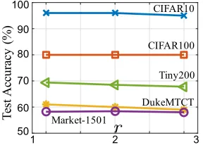
Parameter Analysis. We analysed the parameter sensitivity of HS (min Eq (5)) and SS (rin Eq (6)) designs. Fig 6 shows that a good selection ofmis important, and a high value of mis preferred for object classification but hurts the perfor-mance of person re-id. This is consistent with the earlier observation that re-id needs to mine fine-grained discrimina-tive information by concentrating the learning attention more on the most confusing negative classes. As shown in Fig 7,r is not sensitive to the model performance (r= 2in the main

experiments), rendering SS a favourable choice over HS in terms of parameter selection.

1 1.5 2 2.5 3 50 60 70 80 90 100 CIFAR10 CIFAR100 Tiny200 DukeMTCT Market-1501 3 2 1 60 70 80 90 Te st A cc ur ac y (% )

(b) Positive class loss

(c) Negative class loss

0

2

4

6

8

Training iterations

₁₀

4

0

10

20

30

40

Gradient ratio

₀

20

30

40

0

2

6 x10

4

10

4

500 1000 1500 2000 0

50 100

500

1000

1500

500 1000 1500 2000 10 20 30

0

2000

0

50

100

10

20

30

(a) Overall loss

(d) Gradient ratio

0

500

Training iteration

0

50

100

150

Negative classes loss

100

0

50

250

0

500

LR

SS-LR

150

0

1000

2000

Training iteration

2

4

Negative classes loss

0

1000

2000

2

4

0

Training iteration

Figure 2: Model collapse at early training stage.

where the hard selection function

f

hs

(

m

|

p

, y

)

returns the top

m

%

negative classes with highest

162

prediction probabilities. We also adjust the balancing weight

↵

, inspired by cost-sensitive imbalance

163

learning formulation [65, 44] The weight

↵

can be intuitively set as inversely proportional to the

164

selected negative class number:

↵

=

_b

_m

_%(

_K

₁₎

_c

where

is a hyper-parameter (

= 10

in our

165

experiments). We call this

negative class Hard Selection

based LR formulation as

HS-LR.

166

It is worth pointing out that a smaller

m

will lead to that fewer negative classes learn from the training

167

sample

x

, whilst the others do not learn in a mini-batch training of a deep network. Hence, it reduces

168

the utilisation of training data in each iteration and leads to slow convergence rate and the need for

169

more learning iterations.

170

4.3 Focus Rectification by Negative Class Soft Selection

171

An alternative to HS-LR is soft selection of negative classes. Formally, we add a hardness (probability)

172

adaptive weight

(

p

k

)

r

to each negative class as

173

L

ss

LR

(

x

) =

log(

p

y

)

↵

K

X

k

=1

,k

₆

=

y

⇣

(

p

k

)

r

log(1

p

k

)

⌘

(7)

where

r

0

is the attending parameter that controls the rate of attending hard classes and disregarding

174

easy classes. We set

↵

=

_K

₁

since all negative classes are considered.

175

Our soft selection mechanism achieves hard class mining in this manner: If a negative class

k

is a hard

176

class w.r.t.

x

and receives a higher probability

p

k

, its weight

(

p

k

)

r

is larger and hence more attention

177

is assigned. When the value of

p

k

is small which suggests an easy negative class, the learning

178

attention will be close to 0 and the objective quantity of class

k

is significantly down-weighted. We

179

call this

negative class Soft Selection

based LR formulation as

SS-LR.

180

With SS-LR, we overcome the per-batch lower utilisation limitation of hard selection (Eq (6)). The

181

soft attention principle has also been exploited in other optimisation methods, e.g. Entropy-SGD

182

[66] and focal loss [25]. Entropy-SGD tackles a different problem of seeking better local minima

183

in the model configuration space. Focal loss is more similar to SS-LR (Eq (7)) but with a number

184

of fundamental differences: (1) Focal loss solves the

global

training data sample imbalance whilst

185

SS-LR deals with the

local

sample-wise negative class distraction, regardless whether the global

186

training data is class balanced or not. (2) Focal loss is built on softmax regression, whilst SS-LR is

187

formulated based on logistic regression. (3) Focal loss aims to suppress easy training instances in

188

sample space whilst SS-LR handles the sample-wise negative classes in class space.

189

5 Experiments

190

We evaluated the proposed methods on single-label object classification (Sec 5.1), person instance

191

identification (Sec 5.2) and multi-label clothing attribute recognition (Sec 5.3). It is worth noting that,

192

outperforming existing best results using extra techniques is not the focus of our evaluations. Rather,

193

the key is to investigate the generalisation performance of the same network model learned by two

194

categories of algorithms, SR and LR (Sec 3 and 4).

195

50 100

Figure 7: Sensitivity evaluation ofγin SS-LR.

Hard Mining for SR. How is the performance of the pro-posed focus rectified hard mining on SR? We additionally applied the same HS formulation (Eq (5)) to SR, and tested two cases: (1) With MobileNet on DukeMTMC, we obtained 54.9%/34.9% Rank-1/mAP vs 57.0%/35.8% by the standard

SR. (2) With WRN-28-10 on CIFAR100, no performance change, both at 80.0%. This suggests SR does not suffer from the same NCD problem as LR.

Conclusion

In this work, we have extensively investigated the validity and advantages of the logistic regression (LR) learning al-gorithms for training single-label multi-class neural network classifiers, a standard technique conventionally employed for multi-label classification model learning. This is moti-vated by our in-depth analyses of softmax regression (SR) and LR in learning properties and their correlation. We iden-tified the negative class distraction problem and proposed two rectification solutions using a hard mining idea. Exten-sive experiments on both coarse-grained object classification and fine-grained person re-identification and spare attribute recognition tasks show the performance effectiveness of the proposed LR algorithms over the standard choice SR.

Acknowledgements

This work was partly supported by the China Scholarship Council, Vision Semantics Limited, the Royal Society New-ton Advanced Fellowship Programme (NA150459), and In-novate UK Industrial Challenge Project on Developing and Commercialising Intelligent Video Analytics Solutions for Public Safety (98111-571149).

References

Abadi, M.; Barham, P.; Chen, J.; Chen, Z.; Davis, A.; Dean, J.; Devin, M.; Ghemawat, S.; Irving, G.; Isard, M.; et al. 2016. Tensorflow: A system for large-scale machine learning. In

OSDI.

Akbani, R.; Kwek, S.; and Japkowicz, N. 2004. Applying support vector machines to imbalanced datasets. InECML. Belkin, M.; Niyogi, P.; and Sindhwani, V. 2006. Manifold regularization: A geometric framework for learning from labeled and unlabeled examples. JMLR7(Nov):2399–2434. Bishop, C. M. 2006. Pattern recognition and machine learn-ing (information science and statistics).

Bridle, J. S. 1990. Probabilistic interpretation of feedforward classification network outputs, with relationships to statistical pattern recognition. InNeurocomputing.

Chaudhari, P.; Choromanska, A.; Soatto, S.; LeCun, Y.; Bal-dassi, C.; Borgs, C.; Chayes, J.; Sagun, L.; and Zecchina, R. 2016. Entropy-sgd: Biasing gradient descent into wide valleys. InICLR.

Chua, T.-S.; Tang, J.; Hong, R.; Li, H.; Luo, Z.; and Zheng, Y. 2009. Nus-wide: a real-world web image database from national university of singapore. InCIVR.

Deng, J.; Dong, W.; Socher, R.; Li, L.-J.; Li, K.; and Fei-Fei, L. 2009. Imagenet: A large-scale hierarchical image database. InCVPR.

Dong, Q.; Gong, S.; and Zhu, X. 2017a. Class rectification hard mining for imbalanced deep learning. InICCV. Dong, Q.; Gong, S.; and Zhu, X. 2017b. Multi-task curricu-lum transfer deep learning of clothing attributes. InWACV.

Dong, Q.; Gong, S.; and Zhu, X. 2018. Imbalanced deep learning by minority class incremental rectification.TPAMI. Girshick, R. 2015. Fast r-cnn. InICCV.

Goodfellow, I.; Bengio, Y.; and Courville, A. 2016. Deep learning. MIT press Cambridge.

He, H., and Garcia, E. A. 2009. Learning from imbalanced data.TKDE.

He, K.; Zhang, X.; Ren, S.; and Sun, J. 2016. Deep residual learning for image recognition. InCVPR.

Heinze, G., and Schemper, M. 2002. A solution to the problem of separation in logistic regression. Statistics in medicine.

Howard, A. G.; Zhu, M.; Chen, B.; Kalenichenko, D.; Wang, W.; Weyand, T.; Andreetto, M.; and Adam, H. 2017. Mo-bilenets: Efficient convolutional neural networks for mobile vision applications.arXiv preprint arXiv:1704.04861. Huang, C.; Li, Y.; Change Loy, C.; and Tang, X. 2016. Learning deep representation for imbalanced classification. InCVPR.

Huang, G.; Liu, Z.; Van Der Maaten, L.; and Weinberger, K. Q. 2017. Densely connected convolutional networks. In

CVPR.

Japkowicz, N., and Stephen, S. 2002. The class imbalance problem: A systematic study. IDA.

King, G., and Zeng, L. 2001. Logistic regression in rare events data.Political analysis.

Kingma, D., and Ba, J. 2015. Adam: A method for stochastic optimization. InICLR.

Krishnapuram, B.; Carin, L.; Figueiredo, M. A.; and Hartemink, A. J. 2005. Sparse multinomial logistic regres-sion: Fast algorithms and generalization bounds.TPAMI. Krizhevsky, A., and Hinton, G. 2009. Learning multiple lay-ers of features from tiny images.Technical report, University of Toronto.

Krizhevsky, A.; Sutskever, I.; and Hinton, G. E. 2012. Ima-genet classification with deep convolutional neural networks. InNIPS.

LeCun, Y.; Boser, B.; Denker, J. S.; Henderson, D.; Howard, R. E.; Hubbard, W.; and Jackel, L. D. 1989. Backpropagation applied to handwritten zip code recognition.NC.

Lin, T.-Y.; Goyal, P.; Girshick, R.; He, K.; and Doll. 2017. Focal loss for dense object detection. InICCV.

Lin, M.; Chen, Q.; and Yan, S. 2014. Network in network. InICLR.

Little, W. A. 1974. The existence of persistent states in the brain. InFrom High-Temperature Superconductivity to Microminiature Refrigeration.

Liu, Z.; Luo, P.; Qiu, S.; Wang, X.; and Tang, X. 2016. Deep-fashion: Powering robust clothes recognition and retrieval with rich annotations. InCVPR.

Luce, R. D. 2005.Individual choice behavior: A theoretical analysis.

Maas, A. L.; Hannun, A. Y.; and Ng, A. Y. Rectifier nonlin-earities improve neural network acoustic models. InICML.

Mor-Yosef, S.; Samueloff, A.; Modan, B.; Navot, D.; and Schenker, J. G. 1990. Ranking the risk factors for cesarean: logistic regression analysis of a nationwide study. Obstetrics and gynecology.

Peterson, C., and S¨oderberg, B. 1989. A new method for mapping optimization problems onto neural networks. IJNS. Qiu, Z.; Li, H.; Su, H.; Ou, G.; and Wang, T. 2013. Logistic regression bias correction for large scale data with rare events. InICADMA.

Ristani, E.; Solera, F.; Zou, R.; Cucchiara, R.; and Tomasi, C. 2016. Performance measures and a data set for multi-target, multi-camera tracking. InECCV workshop on Benchmarking Multi-Target Tracking.

Russakovsky, O.; Deng, J.; Su, H.; Krause, J.; Satheesh, S.; Ma, S.; Huang, Z.; Karpathy, A.; Khosla, A.; Bernstein, M.; et al. 2015. Imagenet large scale visual recognition challenge.

IJCV.

Schaefer, R. L. 1983. Bias correction in maximum likelihood logistic regression.Statistics in Medicine.

Srivastava, N.; Hinton, G. E.; Krizhevsky, A.; Sutskever, I.; and Salakhutdinov, R. 2014. Dropout: a simple way to prevent neural networks from overfitting.JMLR.

Weiss, G. M. 2004. Mining with rarity: a unifying framework.

ACM SIGKDD Explorations Newsletter.

Zagoruyko, S. e. a. 2016. Wide residual networks. arXiv preprint arXiv:1605.07146.

Zheng, L.; Shen, L.; Tian, L.; Wang, S.; Wang, J.; and Tian, Q. 2015. Scalable person re-identification: A benchmark. In

ICCV.