Cataract Detection

(1)

711 Copyright © 2011-15. Vandana Publications. All Rights Reserved.

Volume-5, Issue-3, June-2015

International Journal of Engineering and Management Research

Page Number: 711-716

Economic Dispatch Scheduling using Classical and Newton Raphson

Method

Navneet Kaur1, Maninder2, Inderjeet Singh3

1,2,3

Electrical Engineering & PTU, INDIA

ABSTRACT

Over the past several years, concerns have been raised over the possibility that the exposure to 50.60 Hz electromagnetic fields from power lines, substations and other power sources may have detrimental health effects on living organisms. The economic dispatch problem was defined so as to determine the allocation of electricity demand among the committed generating units to minimize the operating costs subject to physical and technological constraints. Economic load dispatch is an important optimization task in power system operation for allocating generation among the committed units such that the system constraints imposed are satisfied and energy requirement in terms of kCal/h or Btu/h or Rupees per hour (Rs/h) are minimized. To all intents and purposes, there has been concern that the economic dispatch may not be the best environmentally. In this research paper economic scheduling of thermal units has been done. Over and above, regular electric supply is the sheer necessity for growing industry and other fields of life.

Keywords--- Economic dispatch, Lamda iteration, Classical Method and Newton Raphson Method.

I. INTRODUCTION

The economic load dispatch problem pertains to the optimum generation scheduling of available generating units in a power system to minimize the cost of generation subject to system constraints [1,2]. In view of rapid growth in demand and supply of electricity, electric power system is becoming increasingly larger and more complex day by day. Regular electric supply is the utmost necessity for growing industry and other fields of life. With the increasing dependence of industry, agriculture and day-to-day household comfort upon the continuity of electric supply, the reliability of power systems has put on great importance [3]. Every electric utility is normally under

obligation to provide to its consumers a certain degree of continuity and quality of service (power flow on transmission lines in a specified range). Therefore, economy, emission etc. objectives of the power system must be properly coordinated in arriving at optimal power dispatch[4,5]. It is, therefore, required to search for better and realistic strategies to achieve various objectives along with desired quality of power supply and satisfying simultaneously various system constraints. This implies economic load dispatch scheduling aspects of the system operation, which are duly investigated in the present work in a unified multiobjective approach[6].

II. ECONOMIC DISPATCH

(2)

712 Copyright © 2011-15. Vandana Publications. All Rights Reserved.

Fig. 2.1 Operating cost versus power output curve

The power output of the plant is increased sequentially by opening a set of valves at the inlet to its steam turbine. The throttling losses in a valve are large, when it is just opened and small when it is fully opened. As a result the operating cost of a plant has the form as shown in Figure. 2.2.

MW (min)

MW (max) Power Output

( Y- axis -Operating cost Rs/h )

Figure 2.2 Cost Rs/h versus output MW curve

For dispatching purposes, this operating cost per unit generator is usually approximated by quadratic polynomial.

( )

(

_i

)

i g i i g i i g

i

P

a

P

b

P

c

F

=

2

+

Rs. /h

Where

a

i

,

b

i

,

c

i are the cost coefficients and i stands for the unit’s number.

The main objective of the economic dispatch is to minimize the cost of fuel for the thermal power system, subject to certain constraints as generating enough power to meet the load demand and to stay within operating

limits [8,9]. Mathematically, this is an optimization problem.

III. SOLUTION BASED ON

LAMBDA ITERATION METHOD

The economic dispatch problem is defined as that which minimizes the total operating cost of the power system while meeting the total load plus transmission losses within generator limits. Mathematically, the problem is defined a

Minimize

( )

_∑

(

)

=

+

=

N

i

i gi i gi i

gi

a

P

b

P

c

P

F

1 2

Rs/h

(3.1a) Subject to

(i) The energy balance equation

∑

=

+

=

N

i

L D gi

P

1

(3.1b) (ii) and the inequality constraint

P

_gimin

≤

P

_gi

≤

P

_gimax

;

(

i

=

1 ,

2 ,...,

N

)

(3.1c)

Where

ai ,bi, ci are the cost coefficients

PD

is the load demand

gi

P

is the real power generation and will act as decision variable

N is the number of generation buses PL

∑∑

= =

=

N

i N

j

gj ij gi

L

P

B

P

1 1

is the transmission power loss.

One of the most important, simple but approximate method of expressing transmission loss as a function of generator powers is through B-coefficients. This method uses the fact that under normal operating conditions, the transmission loss is quadratic in the injected bus real powers. The general form of the loss formula using B-coefficients is

MW

(3.2)

Where, Pgi and Pgj are the real power injections at

the ith and jth buses, respectively

Bij are the loss coefficients which are constant

under certain assumed conditions, N is number of generation buses.

The transmission loss formula of (3.2) is known as George’s formula.

(3)

713 Copyright © 2011-15. Vandana Publications. All Rights Reserved.

∑∑

∑

= = =

+

=

N

i N

j

gj ij gi N

i

gi i

L

B

P

B

P

1 1 1

0

00

MW (3.3) Where

Pgi and

P

gj are the real power injections at ith and jth buses, respectively

B00, Bi0 and Bij are the loss coefficients which are

constant under assumed conditions,

N is the number of the generation buses.

The above constrained optimization problem is converted into an unconstrained optimization problem. Lagrange multiplier method is used in which the function is minimized (or maximized) with side conditions in the form of equality constraints. Using Lagrange multipliers and augmented function is defined as

N

L (Pgi, λ) = F (Pgi) + λ (PD+PL - ∑ Pgi)

(3.4) i=1

Where λ is the Lagrangian multiplier.

Necessary conditions for the optimization problem are

∂L(Pgi, λ )/ ∂Pgi = ∂F(Pgi)/ ∂Pgi+ λ (∂PL /∂Pgi

-1) =0 (i=1,2,…….N) Rearranging the above equation,

∂F(Pgi)/ ∂Pgi= λ (1-∂PL/∂Pgi) (i=1,2,…..N)

(3.5) Where

∂F(Pgi)/ ∂Pgi is the incremental cost of the ith

generator (Rs/MWh)

∂PL/∂Pgi is the incremental transmission losses.

Equation (3.5) is known as the exact coordination equation, and

N

∂L(P gi, λ ) / ∂λ =P D +PL - ∑ Pgi = 0

(3.6)

i=1

Equation (3.5) the so-called coordination equation, numbering N is solved simultaneously with Eqn.

(3.6) to yield a solution for Lagrange multiplier λ and the

optimal generation of N generators., By differentiating the transmission loss equation Eqn (3.3) with respect to Pgi,

the incremental transmission loss can be obtained as, N

∂PL/∂Pgi = Bi0 +∑ 2BijPgj (i=1,2,……..N)

(3.7) j=1

And by differentiating cost function eqn.(3.1a) with respect to Pgi

∂F(P

, the incremental cost can be obtained as

gi)/ ∂Pgi = 2aiPgi +bi

Equation (3.5) can be rewritten as

(i=1,2,…….N) ( 3.8)

{∂F(Pgi)/ ∂Pgi } / (1- ∂PL/∂Pgi)= λ

or

{∂F(Pgi)/ ∂Pgi}Li= λ (i=1,2,…….N)

(3.9)

where Li = 1.0/(1-∂PL/∂Pgi) is called the penalty factor of

ith plant.

To obtain the solution, substitute Eqs. (3.7) and (3.8) into eq (3.5)

N

2aiPgi +bi = λ (1-Bi0 – ∑2BijPgj)

(i=1,2,……..N)

j=1

Rearranging the above equation to get Pgi, we have

N

2(ai+ λ Bii) Pgi =λ (1-Bi0 – ∑ 2Bij Pgj) - bi

(i=1,2,…….N)

j=1 j≠i

The value of Pgi

N can obtained as

Pgi= {λ (1-Bi0 – ∑2 Bij Pgj)-bi} / 2(ai +λ Bii)

(i=1,2,…..N) (3.10) j=1 j≠i

If the intial values of Pgi(i=1,2,…..N) and λ are

known the above equation can be solved iteratively until

eq.(3.6) is satisfied by modifying λ. This technique is

known as successive approximation.

IV. ALGORITHM: ECONOMIC

DISPATCH (CLASSICAL METHOD)

1. Read data, namely cost coefficients, ai, bi, ci;

B-coefficients, Bij, Bi0, B00 (i=1,2,….N ; j=1,2,…….N);

convergence tolerance є, step size α , and maximum

iterations allowed, ITMAX,etc.

2. Compute the initial values of Pgi(i=1,2,……..N) and λ

by assuming that the transmission losses are zero, i.e. PL

=0

3. Set iteration counter, IT =1

4. Compute Pgi (i=1,2…….N) using eq.(3.10)

5. Compute transmission loss using Eq. (3.3) N

6. Compute ∆P= PD +PL – ∑Pgi

i=1

7. Check |∆P| ≤ ε ,if ‘yes’, then GOTO Step 10.

(4)

714 Copyright © 2011-15. Vandana Publications. All Rights Reserved.

8. Update λnew=λ+α|∆P|, where α is the step size u sed to

increase or decrease the value of λ in order to meet the

step 6.

9. IT =IT+1, λ= λnew and GOTO Step 4 and repeat.

10. Compute optimal total cost from eq.(3.1a) and transmission loss from (3.3).

11. Stop.

V. ECONOMIC DISPATCH USING

NEWTON-RAPHSON METHOD

The economic dispatch problem is expressed by eqs.(3.1a), (3.1b) and (3.1c) and is converted into an unconstrained optimization problem as in eq.(3.4) . Necessary conditions for the optimization problems eq.(3.4) are given by eqs. (3.5) and eqs (3.6). The solution of nonlinear eq.(3.5) can be obtained using the Newton-Raphson method in which any change in control variables about the initial values can by obtained using Taylor’s expansion. Taylor’s expansion to second order of eq. (3.5) and eq. (3.6) can be written as

N

(∂2L/ ∂P2gi) ∆Pgi + ∑ (∂2L /∂Pgi∂ Pgj ) Pgj + (∂2L /∂Pgi∂

λ) ∆ λ = -∂L /∂ Pgi (5.1)

j=1 j ≠ i N

∑ ((∂2

L /(∂ λ ∂ Pgj ) ∆ Pgj + (∂2L /∂ λ2

∇ pg pg ∇pgλ ∆pg = -∇pg

∇

) ∆ λ = -∂L /∂ λ (5.2)

j=1

The above equation can be rewritten in matrix form as

T_λ

pg ∇λλ ∆ λ -∇λ

(5.3)

Derivatives can be obtained as follows: ∂L/ ∂Pgi =∂Fi/ ∂Pgi + λ [(∂PL/ ∂Pgi) –1]

N

=(2 ai Pgi+bi) + λ (Bi0 + ∑ 2 Bij Pgj -1)

i=1 (i=1,2,……..N) (5.4a)

N

∂L/ ∂ λ = PD + PL - ∑ Pgi

(5.4b) i=1

Taking derivatives of eq.(3.14a) with respect to Pgi ,

(∂2L/ ∂P 2gi ) =∂ 2Fi/ ∂P 2gi+ λ(∂2 PL/ ∂P 2gi ) =2 ai+2λ Bii

(i=1,2,……NG) (5.5 a)

(∂2L/∂Pgi∂Pgj) = λ (∂2

(i=1, 2 ….NG; j=1,2,…..NG; i≠j) (5.5b)

PL /∂Pgi∂Pgi) =2 λ Bij

Taking derivatives of eqs. (3.14a) and (3.14 b) with

respect to λ ,

NG (∂2L/∂ λ ∂Pgi)= (∂2L/ ∂Pgi∂ λ) = ∂PL/∂Pgi -1=Bi0 +∑ 2 Bij

Pgj-1

i=1

(i=1,2,…..NG) (5.5c)

∂2L/∂ λ2

1. Read data, namely ai, bi, ci (cost coefficients); Bij,

Bi0, B00(B-coefficients) (i=1,2,….N; j=1,2,……N)

convergence tolerance, є, and ITMAX (

maximum allowed iterations), etc.

=0 (5.5d)

Equations (5.1) and (5.2) are iterated till no further improvement is obtained or single derivatives with respect to control variables become zero.

VI. ALGORITHM: ECONOMIC

DISPATCH (NEWTON-RAPHSON

METHOD)

2. Compute the initial values of Pgi (i=1,2,…….,N)

and λ by presuming that PL = 0.

3. Assume that no generator has been fixed either at lower limit or at upper limit.

4. Set iteration counter IT =1.

5. Compute Hessian and Jacobian matrix elements using eqs (3.14) and (3.15)

[H] ∆pg = - [J]

∆ λ

Deactivate row and column of Hessian matrix and row of Jacobian matrix

representing the generator whose generation is fixed either at lower limit or at

upper limit. This is done so that fixed generators,can not participate in allocation.

6. Gauss elimination method is employed in which triangularization and back-

substitution processes are performed to find Pgi

(i=1,2,.. .R and ∆ λ) . Here R is the number of generators which can participate in allocation.

7. Check either

( )

λ



≤

ε











_∇

₊

_∇

∑

=

R

i gi

P

1

2 2

or

ε

λ



≤























∂

+













∂

∑

=

R

i gi

L

P

1

(5)

if convergence condition is ‘yes’ then GOTO Step 10.

Check IT > ITMAX, if condition is ‘yes’ GOTO Step 10.(it means the procedure

proceeds without obtaining required convergence). 8. Modify control variables,

Pgi(new) =Pgi +∆Pgi; (i=1,2,………..R ) and λ (new)

= λ +∆λ

9. IT =IT+ 1, Pgi = Pgi(new) , λ = λ (new) and GOTO

Step 5 and repeat.

10. If no more violations then GOTO Step 12, else check the limits of generators

and fix up as follows:

If Pgi < Pmingi then Pgi = Pmingi

If Pgi > Pmaxgi then Pgi = Pmaxgi

11. GOTO Step 4 and repeat.

12. Compute the optimal total cost and transmission loss.

13. Stop.

VII. TEST SYSTEMS AND RESULTS

7.1 Test problem no.1

The fuel inputs per hour of two plants are given as

F1 (Pg1) = (0.00889 Pg12 +10.333 Pg1 +200) Rs/h

F2 (Pg2) = (0.00741 Pg22 +10.833 Pg2 +240) Rs/h

Determine the economic schedule to meet the demand of 150MW and the corresponding cost of generation. The transmission losses are given by

PL = 0.001Pg12 + 0.002 Pg22

I T

– 2(0.0002 Pg1 P g2 )

Assumptions: α = 0.05, ε =0.0001, and ITMAX=

50

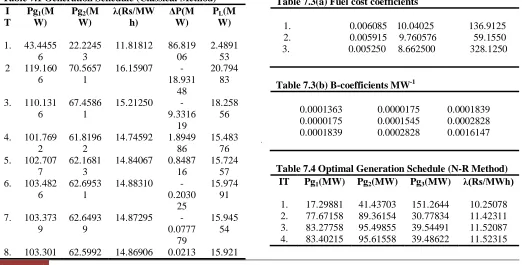
Table 7.1 Generation Schedule (Classical Method) Pg1(M

W)

Pg2(M

W)

λ(Rs/MW h)

ΔP(M W)

PL(M

W)

1. 43.4455 6

22.2245 3

11.81812 86.819 06

2.4891 53 2 119.160

6

70.5657 1

16.15907 -18.931

48

20.794 83

3. 110.131 6

67.4586 1

15.21250 -9.3316

19

18.258 56

4. 101.769 2

61.8196 2

14.74592 1.8949 86

15.483 76 5. 102.707

7

62.1681 3

14.84067 0.8487 16

15.724 57 6. 103.482

6

62.6953 1

14.88310 -0.2030

25

15.974 91

7. 103.373 9

62.6493 9

14.87295 -0.0777

79

15.945 54

8. 103.301 62.5992 14.86906 0.0213 15.921

2 9 91 84

9. 103.313 3

62.6048 5

14.87013 0.0070 19

15.925 22 10

.

103.320 1

62.6095 7

14.87049 -0.0022

29

15.927 43

11 .

103.318 8

62.6089 3

14.87037 -0.0006

37

15.927 05

12 .

103.318 1

62.6084 8

14.87034 0.0002 26

15.926 85 13

.

103.318 3

62.6085 5

14.87035 0.0000 66

15.926 88

TOTAL COST = 2309.77 Rs/hr.

Table 7.2 Generation Schedule (N-R Method) IT Pg1(MW) Pg2(MW) λ(Rs/MWh)

1. 104.5631 60.62549 14.7952 2. 103.2330 62.56359 14.86603 3. 103.3040 62.61016 14.86981 4. 103.3183 62.60859 14.87035

POWER LOSS = 15.9269 MW TOTAL COST = 2309.771 Rs/hr.

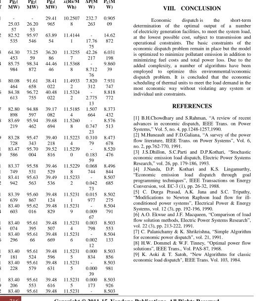
7.2 Test problem no.2

For a three generator system the fuel cost coefficients are given in table 3.3(a). The B coefficients for transmission loss are given in table 3.3(b).Determine the economic schedule for load of 210 MW.

Table 7.3(a) Fuel cost coefficients

Table 7.3(b) B-coefficients MW

0.0001363 0.0000175 0.0001839 -1

0.0000175 0.0001545 0.0002828 0.0001839 0.0002828 0.0016147

Table 7.4 Optimal Generation Schedule (N-R Method) IT Pg1(MW) Pg2(MW) Pg3(MW) λ(Rs/MWh)

1. 17.29881 41.43703 151.2644 10.25078 2. 77.67158 89.36154 30.77834 11.42311 3. 83.27758 95.49855 39.54491 11.52087 4. 83.40215 95.61558 39.48622 11.52315

(6)

POWER LOSS = 8.50394 MW

Table 7.5 Generation Schedule (Classical Method) I

T Pg1(

MW) Pg2(

MW) Pg3(

MW)

λ(Rs/M Wh)

ΔP(M W)

PL(M

W)

1 -25.03 57 -26.20 53 29.41 965 10.2507 8 232.7 263 0.905 09

2 82.52 535 95.97 546 63.89 54 11.4144 1 -17.76 75 14.62 872

3 64.30 453 73.25 59 36.20 86 11.3255 7 42.26 217 6.031 198 4 85.75

984 98.34 872 44.46 46 11.5368 8 -8.712 76 9.860 39

5 80.08 464 91.61 658 38.41 022 11.4933 2 7.820 312 7.931 747 6 84.38

613 96.72 755 40.48 022 11.5324 2 -2.775 13 8.818 772

7 82.80 898 94.88 597 39.17 082 11.5185 4 1.507 664 8.373 432 8 83.69

219 95.94 462 39.68 694 11.5260 8 -0.747 23 8.576 513

9 83.28 728 95.47 343 39.40 218 11.5223 4 0.310 79 8.473 678 1 0 83.47 586 95.70 004 39.52 816 11.5239 0 -0.183 59 8.520 476 1 1 83.37 749 95.58 531 39.46 529 11.5229 8 0.068 744 8.496 844 1 2 83.41 942 95.63 563 39.49 536 11.5233 2 -0.042 73 8.507 685 1 3 83.39 639 95.60 867 39.48 124 11.5231 1 0.015 977 8.502 275 1 4 83.40 603 95.62 016 39.48 829 11.5231 9 -0.009 67 8.504 791 1 5 83.40 074 95.61 395 39.48 507 11.5231 4 0.003 798 8.503 553 1 6 83.40 296 95.61 66 39.48 669 11.5231 6 -0.002 12 8.504 133 1 7 83.40 181 95.61 524 39.48 596 11.5231 5 0.000 834 8.503 856 1 8 83.40 228 95.61 579 39.48 631 11.5231 5 -0.000 39 8.503 981 1 9 83.40 206 95.61 553 39.48 616 11.5231 5 0.000 173 8.503 926 2 83.40 95.61 39.48 11.5231 - 8.503

0 217 564 624 5 0.000 09

952

VIII. CONCLUSION

Economic dispatch is the short-term determination of the optimal output of a number of electricity generation facilities, to meet the system load, at the lowest possible cost, subject to transmission and operational constraints. The basic constraints of the economic dispatch problem remain in place but the model is optimized to minimize pollutant emission in addition to minimizing fuel costs and total power loss. Due to the added complexity, a number of algorithms have been employed to optimize this environmental/economic dispatch problem. It is concluded that the economic scheduling of thermal units to meet the load demand in the most economic way without violating any system or individual unit constraints.

REFERENCES

[1] B.H.Chowdhary and S.Rahman, “A review of recent advances in economic dispatch, IEEE Trans. on Power Systems,” Vol. 5, no. 4, pp.1248-1257,1990.

[2] M.Huneault and F.D.Galiana, “A survey of the power flow literature, IEEE Trans. on Power Systems”, Vol. 6, no. 2, pp.762-770, 1991.

[3] J.S.Dhillon, S.C.Parti and D.P.Kothari, “Stochastic economic emission load dispatch, Electric Power Systems Research,” vol. 26, pp. 179-186, 1993.

[4] J.Nanda, D.P. Kothari and K.S. Lingamurthy, “Economic emission load dispatch through goal programming techniques”, IEEE Transactions on Energy Conversion, vol. EC-3 (1), pp. 26-32, 1988.

[5] C. Durga Prasad, A.K. Jana and S.C. Tripathy, “Modifications to Newton Raphson load flow for ill-conditioned power systems”, Electrical Power & Energy Systems, vol. 12 (3), pp. 192-196, 1990.

[6] A.O. Ekwue and J.F. Macqueen, “Comparison of load flow solution methods, Electric Power Systems Research”, vol. 22 (3), pp. 213-222, 1991.

[7] C. Palanichamy & K. Shrikrishna, “Simple Algorithm for economic power dispatch”, vol. 21, 1991.

[8] H.W. Dommel & W.F. Tinney, “Optimal power flow solutions”, IEEE Trans., Vol. PAS-87, 1968.