+,−%%./∃0
)1 &∀∀%233∀ 43/53
ABSTRACT
Sequential patterns mining is an important data-mining technique used to identify frequently observed sequential occurrence of items across ordered transactions over time. It has been extensively studied in the literature, and there exists a diversity of algorithms. However, more complex structural patterns are often hidden behind sequences. This article begins with the introduction of a model for the representation of sequential patterns—Sequential Patterns Graph—which motivates the search for new structural relation patterns. An integrative framework for the discovery of these patterns–Postsequential Patterns Mining–is then described which underpins the postpro-cessing of sequential patterns. A corresponding data-mining method based on sequential patterns postpropostpro-cessing is proposed and shown to be effective in the search for concurrent patterns. From experiments conducted on three component algorithms, it is demonstrated that sequential patterns-based concurrent patterns mining provides
an eficient method for structural knowledge discovery.
Keywords: concurrent patterns mining method; patterns, postsequential patterns mining; sequential patterns graph; sequential patterns mining; structural relation
INTRODUCTION
Sequential patterns mining is an important data-mining and pattern-discovery technique
that aims to ind the relationships between occurrences of sequential events and to ind if there are any speciic orders within these oc -currences. It has been extensively studied and
several methods have been proposed (Agrawal & Srikant, 1995; Pei, Han, Mortazavi-Asl, &
Pinto, 2001; Zaki 2001). However, there are
still some challenges within the conventional framework: most methods mine the complete set of sequential patterns and, in many cases, a large set of sequential patterns is not intuitive
Sequential Patterns
Postprocessing for Structural
Relation Patterns Mining
Jing Lu, Southampton Solent University, UK
Weiru Chen, Shenyang Institute of Chemical Technology, China
Osei Adjei, University of Bedfordshire, UK
and not necessarily very easy to understand or use. Also, questions that are usually asked with respect to sequential patterns mining are: What is the inherent relation among sequential patterns? Is there a general representation of sequential patterns? Are there any other novel patterns that can be discovered based on se-quential patterns?
These questions pointed out some obstacles within conventional sequential patterns mining methods and indicated further research direc-tions associated with sequential patterns mining that has inspired this work. Since each sequence can be viewed as a partial order of a subset of events, any partial order can be represented by a directed acyclic graph (Mannila & Meek, 2000). It is then possible to describe a set of sequential patterns using a graphical model called Sequential Patterns Graph, or SPG (Lu,
Adjei, Chen, & Liu,2004; Lu, Adjei, Wang, &
Hussain,2004). SPG acts as a bridge between
a discrete sequences set and a uniied graphical
structure. It is not only a minimal representa-tion of sequential patterns mining results, but it also represents the potential interrelation
among patterns such as concurrent, exclusive
or iterative patterns. The framework for mining
these new structural relation patterns has been
called Postsequential Patterns Mining or PSPM
(Lu, Wang, Adjei, & Hussain,2004).
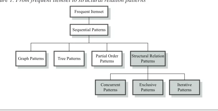
Figure 1 shows the levels of patterns rang-ing from a simple frequent itemset (Agrawal,
Imielinski, & Swami, 1993), to sequential
patterns (Agrawal & Srikant, 1995), to com-plex structures like graph patterns (Ivancsy & Vajk, 2005), tree patterns (Zaki 2002), partial order patterns (Mannila & Meek, 2000), and the proposed structural relation patterns. The
shaded parts in the igure indicate the areas of
new work in this article and elsewhere (Lu,
Wang, et al.,2004; Lu 2006).
The objectives of the research, which has been undertaken (Lu, 2006), are as follows:
• Propose and construct Sequential Patterns
Graph as a new model to represent the relations among sequential patterns.
• Deine new structural relation patterns such
as concurrent patterns, exclusive patterns, and iterative patterns.
• Elucidate the framework for Postsequential
Patterns Mining as an extension of tradi-tional sequential patterns mining.
• Devise methods and develop algorithms
for mining structural relation patterns.
• Demonstrate the effectiveness of the
method, and analyse the eficiency of the
algorithms through experiments.
The remainder of the article is structured as follows: following a summary of sequential
Figure 1. From frequent itemset to structural relation patterns
Graph Patterns Tree Patterns Partial Order Patterns
Structural Relation Patterns Frequent Itemset
Sequential Patterns
Concurrent Patterns
Exclusive Patterns
patterns mining, the Sequential Patterns Graph model is introduced to represent sequential pat-terns graphically. In the next section, structural
relation patterns are deined formally and the
Postsequential Patterns Mining architecture is
described. The focus of this article is on
con-current patterns and an associated data-mining
method, which is then speciied along with its
component algorithms. The penultimate sec-tion gives an experimental evaluasec-tion, using synthetic datasets, and the performance of the algorithms is presented in detail. The article draws to a close by making brief conclusions and indicating future research directions.
SEQUENTIAL PATTERNS
MINING AND MODELLING
Sequential patterns mining aims to discover frequently occurring sequences (or sequential patterns) in a sequence database. It is important to understand the inherent relations among patterns as well as their general representation. Therefore, a graphical model called Sequential
Patterns Graph (Lu, Adjei, Chen, et al., 2004;
Lu, Adjei, Wang, et al., 2004) was proposed
as a model to represent the relations among sequential patterns.
Sequential Patterns Mining
The sequential patterns mining referred to here
is based on frequent itemset mining, which was
originally deined by Agrawal et al.(1993) as fol-lows. Let I={i1,i2,…,il} be a set of l items and let
TDB=<T1,T2,…,Tk> be a transaction database, where Tj (1≤j≤k) is a transaction which contains a set of items in I. Suppose an itemset, denoted by
A=(x1,x2,…,xq), is an unordered nonempty set of
q items. The support (or occurrence frequency)
of A is the number of transactions containing A
in TDB. An itemset A is frequent if A’s support
is no less than a predeined minimum support threshold, . Given a transaction database TDB and a minimum support threshold , the problem
of inding the complete set of frequent itemsets
is called frequent itemset mining.
Following the above concepts for frequent
itemset mining, the problem of discovering
sequential patterns was considered by Agrawal
and Srikant (1995). Their approach introduced
some of the most important and basic deini
-tions in sequential patterns mining. A sequence
S, denoted by <e1 e2… ek>, is an ordered set of
k elements where each element ei (1≤i≤k) is an itemset and k is called the length of the sequence. A sequence databaseSDB is considered to be
a multiset of sequences or, more speciically,
data sequences. A sequence S1=<X1X2 … Xn> is
contained in another sequence S2=<Y1Y2 … Ym> if n≤m and there exist integers 1≤i<i2<…<in≤m
such that Xj⊆
j i
Y(1≤j≤n), and it is denoted by
S1∠S2. If sequence S1 is contained in sequence
S2, then S1 is called a subsequence of S2 and S2
a super-sequence of S1.
The absolute support of sequence Sin
SDB is deined as the number of sequences
belonging to SDB that contain S, and the
relative support is deined as the percentage
of sequences belonging to SDB that contain S.
The relative measure of support will be used throughout this article, where the support of
S in SDB is denoted by S.sup. The minimum
support (minsup) is speciied by the user and
stands for the minimum fraction of total data sequences which support this sequence. A
se-quence S is called a sequential pattern in SDB
if S.sup≥minsup. A sequential pattern is called amaximal sequence if it is not contained in any other sequential patterns.
Using the above deinitions, Agrawal
and Srikant (1995) proposed the problem of sequential patterns mining as follows: given a sequence database SDB, where each sequence consists of a list of elements and each element consists of a set of items, and given a minimum support threshold, sequential patterns mining aims to discover the set of all sequential
pat-terns (SP) in SDB.
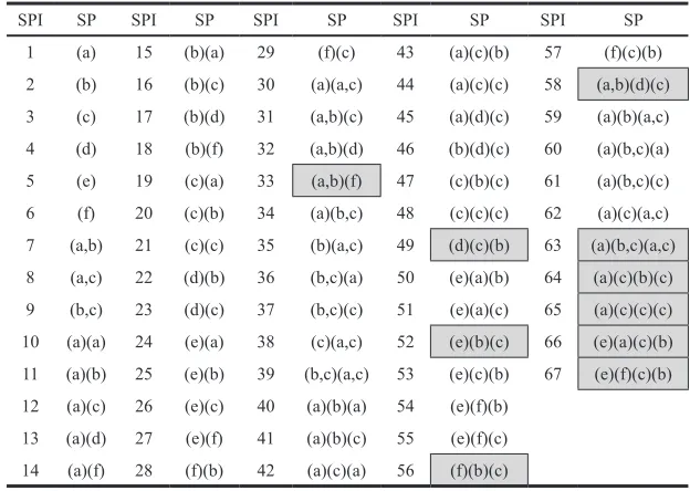
Example 1 Consider a sequential patterns
mining example used in PreixSpan (Pei et al.,
2001): given SDB={<a (a,b,c) (a,c) d (c,f)>, <(a,d) c (b,c) (a,c)>, <(e,f) (a,b) (d,f) cb>, <e g (a,f) cbc>} with a minsup of 50%. Table 1 shows the set of all sequential patterns under
this setup and the Sequential Patterns Index,
Given a SDB and user speciied minsup,
a set of sequential patterns can be discovered from sequential patterns mining. All sequential patterns marked within the boxes in Table 1 are sub-sequences of maximal sequences.
Sequential Patterns Graph
The use of graphs to model complex datasets has been recognised by various researchers in
different domains. In the ield of Knowledge
Discovery, using graphs is an expressive and versatile modelling technique that provides ways to reason about information implicit in the data (Cook & Holder, 2000; Garriga 2005; Lin & Lee, 2005). Typically, nodes of these graphs are sets of items, and edges represent the
rela-tionships of speciicity among them. This has
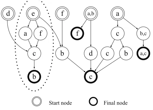
led to the development of a sequential patterns model that explores the inherent relationship among sequential patterns. All sequential pat-terns under minsup can be generated from the maximal sequences. Thus, a directed acyclic Sequential Patterns Graph or SPG [16,17] can be used to represent the maximal sequence sets. Figure 2 shows an SPG that corresponds to the
set of maximal sequences and, therefore, the complete set of sequential patterns in Table 1.
With reference to Figure 2, it is seen that nodes (i.e., items or itemsets) of SPG corre-spond to elements in a sequential pattern and directed edges are used to denote the sequence relation between two elements. Any path from
a start node to a inal node corresponds to one
maximal sequence. Two special types of nodes
called the start node and the inal node are used
to indicate the beginning and end of maximal sequences.
As a further example, consider the segment circled by a dotted line above; it represents maximal sequences <eacb> and <efcb> in particular; it also represents other sequential patterns <e>, <a>, <c>, <f>, <b>, <ea>, <ef>, <ec>, <eb>, <ac>, <fc>, <ab>, <fb>, <cb>, <eac>, <efc>, <eab>, <efb> and <ecb>. Hence, SPG is a summary of sequential patterns, useful
for representing results to users. The deini
-tion, properties and the construction method of SPG are developed systematically in (Lu,
Adjei, Chen, et al.,2004; Lu, Adjei, Wang,et
al.,2004).
SPI SP SPI SP SPI SP SPI SP SPI SP
1 (a) 15 (b)(a) 29 (f)(c) 43 (a)(c)(b) 57 (f)(c)(b)
2 (b) 16 (b)(c) 30 (a)(a,c) 44 (a)(c)(c) 58 (a,b)(d)(c)
3 (c) 17 (b)(d) 31 (a,b)(c) 45 (a)(d)(c) 59 (a)(b)(a,c)
4 (d) 18 (b)(f) 32 (a,b)(d) 46 (b)(d)(c) 60 (a)(b,c)(a)
5 (e) 19 (c)(a) 33 (a,b)(f) 47 (c)(b)(c) 61 (a)(b,c)(c)
6 (f) 20 (c)(b) 34 (a)(b,c) 48 (c)(c)(c) 62 (a)(c)(a,c)
7 (a,b) 21 (c)(c) 35 (b)(a,c) 49 (d)(c)(b) 63 (a)(b,c)(a,c)
8 (a,c) 22 (d)(b) 36 (b,c)(a) 50 (e)(a)(b) 64 (a)(c)(b)(c)
9 (b,c) 23 (d)(c) 37 (b,c)(c) 51 (e)(a)(c) 65 (a)(c)(c)(c)
10 (a)(a) 24 (e)(a) 38 (c)(a,c) 52 (e)(b)(c) 66 (e)(a)(c)(b)
11 (a)(b) 25 (e)(b) 39 (b,c)(a,c) 53 (e)(c)(b) 67 (e)(f)(c)(b)
12 (a)(c) 26 (e)(c) 40 (a)(b)(a) 54 (e)(f)(b)
13 (a)(d) 27 (e)(f) 41 (a)(b)(c) 55 (e)(f)(c)
14 (a)(f) 28 (f)(b) 42 (a)(c)(a) 56 (f)(b)(c)
The signiicance of SPG is not limited to
the minimal representation of a collection of sequential patterns. It also motivates the further relationships among sequential patterns to be discovered. Some sequential patterns may be supported by the same data sequence, and these
are called concurrent patterns; while some
others may not possibly occur in the same data
sequence, and these are called exclusive
pat-terns. Furthermore, some sequential patterns may occur more than once in a data sequence, such that an iterative relationship is expressed, and this is called an iterative pattern. This leads to more complex structured patterns called
structural relation patterns, to be deined for -mally in the next section.
STRUCTURAL RELATION
PATTERNS AND
POSTSEQUENTIAL PATTERNS
MINING
With the successful development of eficient
and scalable algorithms for mining frequent itemsets and sequences, the literature has been extended to other structures like partial order
(Atallah, Gwadera, & Szpankowski, 2004;
Garriga & Balcazar, 2004; Mannila & Meek,
2000), graph (Cook & Holder, 2000; Han &
Yan, 2004; Huan, Wang, Prins, & Yang,2004)
and tree (Zaki, 2002) patterns. The search for
novel patterns deined here can be motivated
using SPG and the framework to mine this new knowledge is known as Postsequential Patterns
Mining (Lu, Adjei, Wang, et al.,2004).
Structural Relation Patterns
For the following deinitions, it is assumed
that {sp1,sp2,…,spm}is the set of m sequential
patterns and they are not contained in each
other.
Deinition 1 Concurrence and Concurrent Patterns: The concurrence of sequential pat-terns sp1,sp2,…,spk (1≤k≤m) is deined as the fraction of data sequences that contain all of the sequential patterns. This is denoted by
concurrence(sp1,sp2,…,spk)=|{C:∀i (i=1,2,…,k)
spi∠C, C∈SDB}|/|SDB| (1)
where spi∠C represents sequential pattern spi contained in data sequence C and the symbol |…| denotes the number of data sequences. Figure 2. A sequential patterns graph of sequential patterns in Table 1
a
c
f
b
c
d
b,c
f
e
d
a,ba
b
c
f
a,c
Start node Final node
Let mincon be the user speciied minimum
concurrence. If
concurrence(sp1,sp2,…,spk)≥mincon
(2)
is satisfied, then sp1,sp2,…,spk are called
concurrent patterns. This is represented by
ConPk=[sp1+sp2+…+spk] where k is the number of sequential patterns which occur together, and the notation ‘+’ represents the concurrent relationship.
Example 2 Consider SDB={<a (a,b,c)
(a,c) d (c,f)>, <(a,d) c (b,c) (a,c)>, <(e,f) (a,b) (d,f) cb>, <eg (a,f) cbc>} and assume a mincon
of 50%. Since both data sequences <(e,f) (a,b) (d,f) cb> and <eg (a,f) cbc> support sequential patterns <ebc>, <eacb> and <efcb>, then:
c o n c u r r e n c e( <e b c> , <e a c b> , <efcb>)=2/4=50%.
Therefore, they constitute a concurrent pattern given by ConP3=[<ebc>+<eacb>+<
efcb>].
The deinition of a sequence contained in
another sequence can be applied to concurrent patterns.
Definition 2 Maximal Concurrent Pat
-terns: Concurrent pattern ConPk=[a1+a2+… +ak] is contained in concurrent pattern ConP(k+m) =[b1+b2+…+bk+m] if ai∠bj, for
1≤i≤k and 1≤j≤(k+m). This is denoted by
ConPk∠ConP(k+m).
Concurrent patterns are called maximal
if they are not contained in any other concur-rent patterns.
In a complementary manner, the
relation-ship between sequential patterns that do not
typically occur together in data sequences can be explored when a maximum exclusion degree
maxexc is speciied.
Deinition 3: Exclusive Patterns: Sequential patterns sp1 and sp2 are called exclusive
pat-terns if
concurrence(sp1,sp2)≤maxexc
(3)
is satisied, and is represented by ExcP=[sp1
–sp2], where the notation ‘–’ represents the exclusive relationship.
The maxexc degree is the extent that sequential patterns are allowed to occur to-gether and remain exclusive. Consider the same sequence database SDB in Example 2 and assume a maxexc of 0. Any data sequence in SDB which contains <a(b,c)(a,c)> does not contain <efcb>, and vice versa. Therefore, the concurrence is zero and an exclusive pattern ExcP=[<a(b,c)(a,c)>–<efcb>] is obtained.
Deinition 4: Iterative Patterns: A sequential pattern sp is known as an iterative pattern if it appears within the same data sequence at least
n times (n ≥ 2) and at most m times (m ≥ n).
The expression <{sp}mn> denotes the iterative
pattern, where m and n represent the upper and lower iteration bounds respectively, which means the maximal and minimal number of patterns appearing in a data sequence. If an iterative pattern has no upper iteration bound, then the parameter m is not required.
As an illustration, consider the SDB of Example 2 again and assume a minsup of 50%;
then an iterative pattern {c}3 can be obtained,
where c is a sequence of length 1, which iterates
three times in the irst two data sequences.
Deinition 5: Structural Relation Patterns
Furthermore, the concurrent, exclusive or iterative combination of structural relation
patterns constitutes new SRPs.
Postsequential Patterns Mining
Having deined structural relation patterns the main problem is to ind a method to mine such
patterns. This subsection will introduce a new approach called postsequential patterns mining,
or PSPM (Lu, Adjei, Wang, et al.,2004), which
is used to provide a framework for mining structural relation patterns.
It is interesting to note that structural relation patterns are often hidden within se-quential patterns. With years of research and
development, there have been many eficient
and scalable sequential patterns mining methods devised. In order to capitalise on these pattern discovery techniques, sequential patterns min-ing is used to drive PSPM. Further analysis of the inherent relationships behind sequential
patterns results in the identiication of more
complex structures—such as concurrent pat-terns, exclusive patterns or iterative patterns—to be discovered.
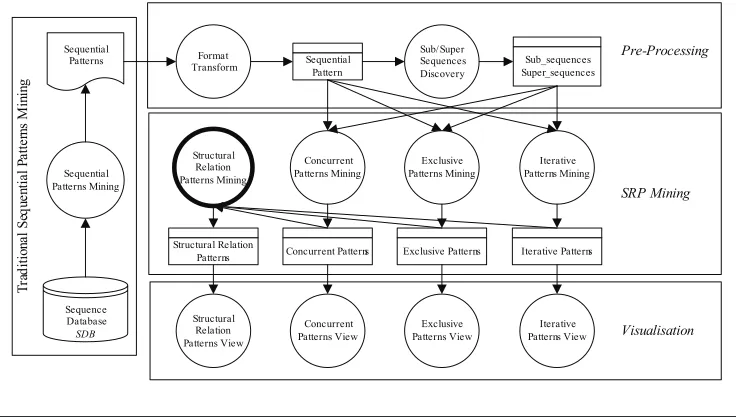
Figure 3 shows the architecture of PSPM and its relationship with traditional sequential patterns mining. It is clear that, in order to
pursue postsequential patterns mining, the traditional sequential patterns mining should
be performed irst (as indicated to the left of the igure). A sequence database provides the
input and sequential patterns are discovered after sequential patterns mining. Postsequential patterns mining can be viewed as a three-phase
process: Preprocessing, SRP Mining and
Vi-sualisation (as indicated from the top to the
bottom of the igure).
The irst Preprocessingtask transforms the result of sequential patterns mining into the ap-propriate format for the system. This phase also
inds the subsequences and supersequences of
each sequential pattern, which is straightforward and necessary for the following phase.
SRP Mining corresponds to the execution of the mining algorithm. This phase is complex and has several challenges that can be charac-terised in principle as follows:
i. Representation of structural relation
pat-terns, including the formal (or logical) representation, computer internal repre-sentation and visual reprerepre-sentation. ii. Development of effective methods to
dis-cover structural relation patterns, based on sequential patterns post-processing.
T ra d it io na l S eq ue nt ia l P at te rn s M in in g Sequential Patterns Mining Sequential Patterns Structural Relation Patterns View Structural Relation Patterns Mining Concurrent Patterns Mining Exclusive Patterns Mining Iterative Patterns Mining
Concurrent Patterns Exclusive Patterns Iterative Patterns Structural Relation Patterns Format Transform Sub/ Super Sequences Discovery Sub_sequences Super_sequences Sequential Pattern Concurrent Patterns View Iterative Patterns View Exclusive Patterns View Pre-Processing Sequence Database SDB SRP Mining Visualisation
iii. Adoption of appropriate data sequences to test the algorithms and analyse their
performance for eficiency.
iv. Understanding of the actual meanings of structural relation patterns, related to the application area of real-world datasets.
During the inal Visualisation phase, the
mined structural relation patterns can be rep-resented graphically, although it is not covered in this article.
CONCURRENT PATTERNS
MINING METHOD AND
ALGORITHMS
Concurrency is an important aspect of some system behaviour. For example, discovering patterns of concurrent behaviour from traces of system events is useful in a wide variety of software engineering tasks, including architec-ture discovery, reengineering, user-interaction modelling, and software-process improvement. The structural relation patterns of particular interest here are concurrent patterns and this section will propose a corresponding data-min-ing method and its three component algorithms, indicating computational complexity.
Concurrent Patterns Mining Method
The three main steps in this method to mine concurrent patterns are described below:
1. Calculation of Sequential Patterns
Sup-ported by Data Sequences (SuppSP)
Sequential patterns which are supported
by a sequence C (i.e., C∈SDB) are computed
and denoted by:
SuppSP(C) ={sp: sp∈SP∧sp∠C}
(4)
T h e u n i o n o f s e t s
SuppSP(C1),SuppSP(C2),…,SuppSP(Cn), where Ci∈SDB (1≤i≤n, n is the number of data sequences in SDB), are the sequential
patterns supported by the sequence database SDB, denoted by:
1
( )
n
i i
SuppSp SuppSP C
−
=
(5)
The detailed algorithms for this step will
be deined in the next section.
2. Determination of Concurrent Patterns
(ConP)
Each SuppSP(Ci) can be viewed as a
transaction (i.e., the unordered set of sequential
patterns supported by data sequence Ci). Thus,
the problem of inding the concurrent patterns which satisfy the user speciied minimum
concurrence (mincon) becomes one of mining frequent itemsets under minsup. Therefore, the traditional frequent itemset mining approach can be adapted for this step.
3. Finding Maximal Concurrent Patterns (MaxConP)
According to the containing relationship among sequences, the ConP need to be
sim-pliied in order to get the maximal concurrent patterns. This can be obtained using Deinition
2 by:
a. Deleting the concurrent patterns which are contained by other concurrent patterns; b. Deleting the sequential patterns in ConP
which are contained by other sequential patterns of the ConP.
Example 3 An example is given to ex-plain how to mine concurrent patterns based on traditional sequential patterns mining. In
order to do this, the sequence database SDBin
Step 1. Using the results from Table 1, SuppSP are computed for every data sequence in order. These results are shown in Table 2, where the column SuppSP lists the sequential patterns index supported by the corresponding
Data Sequence Index, DSI.
Step 2. To calculate concurrent patterns,
consider mincon to be 50%, which means ind -ing the groups of sequential patterns which occur together in more than 50% of the data sequences. Then the frequent itemset mining method is used to discover concurrent patterns with the minimum support threshold set to mincon. The results are listed below:
11 12 16 3 2 1: 4
11 12 16 3 2 1 21 23 41 44 4 65 63 62 61 60 59 48 15 42 40 39 38 37 36 35 34 30 19 10 9 8 : 2
11 12 16 3 2 1 23 4 6 13 14 58 46 45 17 33 32 31 18 7 : 2
11 12 16 3 2 1 20 23 43 4 49 22 : 2
11 12 16 3 2 1 20 43 6 67 66 57 56 55 54 53 52 51 50 5 29 28 27 26 25 24 : 2
11 12 16 3 2 1 20 21 41 43 44 64 47 : 2 11 12 16 3 2 1 6 : 3
11 12 16 3 2 1 21 41 44 6 : 2 11 12 16 3 2 1 23 4 : 3 11 12 16 3 2 1 21 41 44 : 3 11 12 16 3 2 1 20 43 : 3
Each line above represents a concurrent pattern. For example,
11 12 16 3 2 1: 4
means concurrent pattern [11+12+16+3+2+1] and the value after the symbol “:” is the number of sequences which support this concurrent pattern.
Step 3. In the above example, consider the three concurrent patterns underlined in step 2; since
[11+12+16+3+2+1]∠[11+12+16+3+2+1+6]∠[
11+12+16+3+2+1+21+41+44+6],
then neither of the concurrent patterns [11+12+16+3+2+1] and [11+12+16+3+2+1+6] are maximal, and they can be deleted.
One can then ask: is ConP10=[11+12+16
+3+2+1+21+41+44+6] a maximal concurrent pattern now? Further work is still needed and, in this case, the sub-sequence which was calculated during the Preprocessing phase is useful. For
example, for ConP10 and referencing Table 1,
the following contained relationships exist:
1∠11∠41, 2∠11∠41, 3∠11∠41 and 1∠12∠41,
2∠12∠41, 3∠12∠41, 16∠41, 21∠44
Therefore 1,2,3,11,12,16,21 can be
deleted from ConP10, which results in
ConP3=[6+41+44].
Deleting all nonmaximal concurrent pat-terns gives the results below, which show the maximal concurrent patterns (MaxConP).
DSI SuppSP
1 1,2,3,4,6,8,9,10,11,12,15,16,19,20,21,22,23,30,34,35,36,37,38,39,40,41,42,43,44,47,48,49, 59,60,61,62,63,64,65
2 1,2,3,4,5,7,8,11,12,13,14,16,17,18,20,22,23,24,25,26,27,28,29,31,32,33,43,45,46,49,50,51,5 2,53,54,55,56,57,58,66,67
3 1,2,3,4,6,7,8,9,10,11,12,13,14,15,16,17,18,19,21,23,30,31,32,33,34,35,36,37,38,39,40,41,42 ,44,45,46,48,58,59,60,61,62,63,65
[23+63+65] [52+56+66+67] [11+33+58] [16+43+49] [6+41+44]
Using these results and Table 1, the patterns are represented as
[dc+a(b,c)(a,c)+accc] [ebc+eacb+efcb+fbc] [ab+(a,b)f+(a,b)dc] [bc+acb+dcb] [f+abc+acc]
Algorithms
The focus in this sub-section is on the irst step
of the concurrent patternsmining method—how
to calculate sequential patterns supported by data sequence (i.e., SuppSP). Two categories
of algorithms, called Full-Check (FCmine)
and Partial-Check (PCmine), are developed for
mining such sequential patterns. The FCmine algorithm is given below in pseudo-code.
Performance Analysis
In the FCmine algorithm, data sequences are compared with all the sequential patterns.
Therefore, the complexity is O(m×n), where n
is the number of data sequences and m is the
number of sequential patterns.
An alternative category of algorithms,
called Partial-Check (PCmine), is proposed
to mine sequential patterns supported by data sequence. Before addressing this category
concerning SuppSP mining, two lemmas are
presented based on an antimonotone Apriori
property, which states in Agrawal et a l. (1993)
if a pattern with k items is not frequent, any of its superpatterns with (k+1) or more items can never be frequent.
Lemma 1 If a sequential pattern sp is
sup-ported by a data sequence C, then all the
sub-sequences of sp must be supported by C too.
Lemma 2 If a sequential pattern sp is not
supported by a data sequence C, then all the
supersequences of sp cannot be supported by
C either.
PCmine is similar to FCmine in that it also checks the relationship between data sequence and sequential pattern. But it is different from
the latter in that PCmine utilises the above
lem-mas and is able to avoid some comparisons of sequential patterns.
Depending on different usage of the above
two lemmas, the PCmine category can be
di-vided into two algorithms:
TopDown Algorithm (i.e., Lemma1 is used);
BottomUp Algorithm (i.e., Lemma 2 is used).
Both of these algorithms require the use of sub-sequences or super-sequences of se-quential patterns that are calculated during the Preprocessing phase. Since the sub-sequences or supersequences are also used in other phases of the mining, there is no extra computational cost in the use of the algorithms.
The following notation is used to make the proposed algorithm more concise and clear:
Input: Sequence database (SDB); sequential patterns (SP).
Output: Sequential patternssupported by data sequences (SuppSP).
Procedure:
(1) For each data sequence Ci in SDB
(2) {SuppSP(Ci)=∅ // SuppSP(Ci) is the pattern set supported by Ci
(3) For each spk∈SP // k is the identiier of spk and ranges from 1 to the length of SP (4) {If spk∠Ci // spk is contained in data sequence Ci.
• SubSeq(spk): Represents a set of
sub-se-quences of sequential patterns spk
• SupSeq(spk): Represents a set of
superse-quences of sequential patterns spk
• Mark(spk,true): Sets the mark of spkto be
true (i.e., sequential pattern spk is supported by a data sequence)
• Mark(spk,false): Sets the mark of spkto be false (i.e., sequential pattern spk is not supported by a data sequence)
Performance Analysis
The above algorithm makes use of Lemma 1. That is, if a data sequence Ci supports a
sequential pattern spk, then all sub-sequences
of spk (i.e., SubSeq(spk)), are also supported by Ci (see rows (5) and (6) in Algorithm 2).
These sub-sequences of spk need not be checked
further. Therefore, in this approach, only the following two types of sequential pattern need to be checked in order to determine if they are supported by a data sequence:
a. sequential patterns whose supersequences
are not supported by the data sequence;
In this case, given a sequential pattern
sp and for any data sequence C, the minimum
support implies that the extent that sp is not
supported by C is (1-minsup). Clearly for m
sequential patterns the extent will be m×
(1-minsup).
b. sequential patterns which have no super-sequences (i.e., maximal super-sequences)
Compared with the number of sequential patterns, the number of maximal sequences is small. For example, consider a maximal
sequence of length L, where there are 2L-1
sub-sequences and the maximal sequence is just the
fraction 1/(2L-1 +1) of these patterns.
So, generally speaking, most sequential patterns which need to be checked are from case a). This means that the number of sequential
patterns may be computed as m×(1-minsup)
times. On the whole, the complexity of the
TopDown algorithm is O(n×m×(1-minsup))
and itis eficient when minsupis greater than
0.5 and approaches 1.
Performance Analysis
In the BottomUp approach, only the
follow-ing two types of sequential pattern need to be checked in order to determine if they are sup-ported by a data sequence:
a. sequential patterns which have no sub-sequence.
b. sequential patterns whose sub-sequences
are supported by the data sequence.
If a sequential pattern is not supported by a
data sequence, then its supersequences are not
Input: Sequence database (SDB); sequential patterns (SP)
Output: Sequential patterns supported by data sequences (SuppSP)
Procedure:
(1) For each data sequence Ci in SDB (2) {Let SuppSP(Ci) be empty
(3) Clear marks of all sequential patterns
(4) For each spk∈SP // k is the identiier of spk and ranges from the length of SP to 1 (5) {If (no mark on spk)and (spk∠Ci)
(6) {SuppSP(Ci)=SuppSP(Ci)+spk+SubSeq(spk); (7) Mark(spk,true);
(8) Mark(SubSeq(spk),true);} (9) }
either and therefore do not need to be compared against the data sequence.
The complexity of this algorithm is O(n×m×minsup) and it is more eficient when
minsupis smaller, especially when minsup is
less than 0.5 and approaches 0. A small minsup means lower support for sequential patterns from data sequences (i.e., most of the data se-quences will not support a sequential pattern and therefore will not support its supersequences, which is often the case for real applications).
It can be concluded that the complexities of algorithms 1, 2 and 3 increase as the number of
data sequences (n) and the number of sequential
patterns (m) increase. In algorithms 2 and 3 the
complexities depend on the factors (1-minsup)
and minsup respectively; therefore the TopDown
and BottomUp algorithms of PCmine are likely
to be more eficient than FCmine.
The three algorithms described above cor-respond to step 1 of the data-mining method specified in the previous subsection—the calculation of sequential patterns supported
by data sequences (i.e., SuppSP). Any frequent
itemset mining can be used in step 2 to generate concurrent patterns so long as all of the SuppSP have been discovered. SuppSP(Ci), (1≤i≤n), is an unordered set and can be considered as a
transaction Ti in TDB. The minimum support
threshold is taken to be the minimum
concur-rent threshold mincon and the results of this mining—frequent itemsets—are the concurrent
patterns required. An eficient mining technique
called CLOSET (Pei, Han, & Mao,2000) can for
example be used in this step. It is worth noting that the data reduction from step 1 to step 2 is
from O(n×m) to at most O(n).
Finally, maximal concurrent patterns need to be discovered. The key requirement in
step 3 is checking the containing relationship
between sequences, which is straightforward in principle.
EXPERIMENTS
To evaluate the eficiency of the algorithms,
experiments were performed on large-scale synthetic datasets that show consistent and promising results. The performance of the algorithms was measured by comparing their running time on a dedicated computer.
Experimental Set-Up and Datasets
The experiments for concurrent patterns mining were performed on a 2.4GHz Pentium PC, with 1.0GB main memory, running under Microsoft Windows 2000. To make the time measurements more reliable, no other application was allowed to run on the system while the experiments were running.
Input: Sequence database (SDB); sequential patterns (SP)
Output: Sequential patterns supported by data sequences (SuppSP)
Procedure:
(1) For each data sequence Ci in SDB (2) {SuppSP(Ci)=∅
(3) Clear marks of all sequential patterns
(4) For each spk∈SP // k is the identiier of spk and ranges from 1 to the length of SP (5) {If (no mark on spk)
(6) {If (spk∠Ci)
(7) {SuppSP(Ci)=SuppSP(Ci)+spk; (8) Mark(spk,true);}
(9) else
(10) {Mark(spk,false);
Synthetic sequence data used in this experiment were generated using the IBM data generator, which has been used in most sequential patterns mining studies (Agrawal &
Srikant, 1995; Pei et al.,2001; Zaki 2001). The
particular software was retrieved in July 2007 from IBM Almaden (http://www.almaden.ibm. com/cs/projects/iis/hdb/Projects/data_mining/ datasets/syndata.html).
The datasets consist of sequences of item-sets, where each itemset represents a market basket transaction.
This synthetic dataset generator produces a database of data sequences whose character-istics can easily be controlled by the user. The generator allows one to specify the number of data sequences |D|, the average number of
transactions in a sequence |C|, the average length
of maximal potentially large sequences |S|, the
average number of items in a transaction |T|, and the number of different items |N|. Table 3 characterises the test datasets appropriate to this article.
The convention for the datasets can be
described as follows: dataset C10-T8-S8-N
1K-D10K, for example, means that the dataset
contains 10,000 (i.e., 10K) data sequences and the number of items is 1,000 (i.e., 1K). The
average number of items in a transaction (i.e., event) is set to 8, and the average number of transactions per data sequence is set to 10. Using the same convention as noted previously, it is straightforward to deduce the meanings of the other datasets in Table 3. These four synthetic datasets are used to compare the performance of algorithms in mining concurrent patterns.
Calculation of Sequential Patterns Supported by Data Sequence
The respective performance is considered here for the three algorithms proposed in the previous
section for mining SuppSP; that is, the FC (Full
Check mining), TD (TopDown Partial mining)
and BU (BottomUp Partial mining) algorithms.
The experiments use the four synthetic datasets
C10-T8-S8-N1K-D10K, C100-T4-S4-N
100-D100, C100-T4-S4-N100-D100 and C50-T
2.5-S4-N1K-D1K, which are described in Table
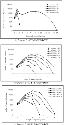
3. The corresponding pattern distributions resulting from mining the above datasets are
listed in Figure 4 (from a to d), which shows
the number of sequential patterns of different lengths for various levels of minsup.
To explain the experimental results, one may distinguish between “dense” datasets and “sparse” datasets. A dense dataset has many frequent patterns of larger size and higher support, while datasets with mainly short pat-terns are called sparse. Longer patpat-terns may exist in sparse datasets, but only with very low support.
It can be seen from Figure 4(a) that the
sequence database C10-T8-S8-N1K-D10K is
sparse. For example, when minsup is 1% or more, the length of sequential patterns is very short (only 2 or 3). From the data distributions
which are shown in Figure 4 (b to d), one may
conclude that datasets C100-T4-S4-N
100-D100, C100-T4-S4-N100-D100 and C50-T
2.5-S4-N1K-D1K are relatively dense.
The three algorithms FC, TD and BU were
all found to be effective in calculation of the sequential patterns supported by data sequences,
Name |C| |T| |S| |N| |D| Size
(KB)
C10-T8-S8-N1K-D10K 10 8 8 1,000 10,000 2540
C50-T2.5-S4-N1K-D1K 50 2.5 4 1,000 1,000 635
C200-T2.5-S4-N1K-D1K 200 2.5 4 1,000 1,000 2520
Figure 4. Pattern distributions from mining synthetic datasets
1 10 100 1000 10000 100000 1000000
1 2 3 4 5 6 7 8 9 10 11 12 13 14 15 16 17
Length of sequential pattern
N
u
m
b
er
o
f
se
q
u
en
ti
al
p
at
te
rn
s
minsup=2.5% minsup=2% minsup=1.5% minsup=1% minsup=0.5%
(a) Dataset C10-T8-S8-N1K-D10K
1 10 100 1000 10000 100000
1 2 3 4 5 6 7
Length of sequential pattern
N
u
m
b
er
o
f
se
q
u
en
ti
al
p
at
te
rn
s
minsup=100% minsup=99% minsup=98% minsup=97% minsup=96% minsup=95%
(b) Dataset C100-T4-S4-N100-D100
1 10 100 1000 10000 100000
1 2 3 4 5 6 Length of sequential pattern
N
u
m
b
er
o
f
se
q
u
en
ti
al
p
at
te
rn
s
minsup=70% minsup=65% minsup=60% minsup=55% minsup=50%
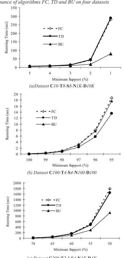
so the analysis presented below is comparing
their eficiency. Figure 5(a-d) demonstrates
the relationship between the running time and the minimum support (minsup) on the four datasets respectively. Note that the running time excludes the data reading time and the result writing time.
The following conclusions are drawn from the experiments on the four datasets.
1. The test results demonstrate that the three algorithms are able to discover all sequen-tial patterns supported by data sequences
(SuppSP) to varying levels of eficiency,
depending on the minimum support (minsup).
2. The FC algorithm is generally less eficient
than the TD and BU algorithms. The rea-son is that FC is based on a full checking approach; therefore, each sequential pat-tern is compared to every data sequence in the database in order to determine if it is supported.
3. The TD algorithm is most eficient (see
Figure 5 (b)) only when minsup is large, for example as it approaches 1. This
conirms its computational complexity
of O(n×m×(1-minsup)) discussed in the
previous section.
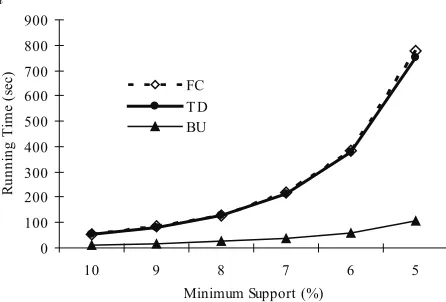
4. The BU algorithm is most eficient (see
Figures 5 (a), (c) and (d)) as minsup be-comes smaller. Computational complexity
of O(n×m×minsup) is again conirmed
from before.
Clearly, the BU algorithm is of most prac-tical value from the above results, especially in real large-scale applications where minsup is typically small. It is also worth noting that, while the TD algorithm starts checking from the largest sequential patterns, BU begins with the shortest, and larger sequential patterns require more items to be compared within the same data sequence and, hence, need more time in general.
CONCLUSION AND FUTURE
WORK
The challenge of mining patterns not only relates to the search for frequent itemsets, but also more and more complex patterns. The work described in this article is intended to develop data-mining techniques in order to discover new structural relations through the postprocessing of sequential patterns. Thus, the main contribu-tions of this article are drawn from three key areas that encompass sequential patterns graph, postsequential patterns mining, and a novel
data-(d) Dataset C50-T2.5-S4-N1K-D1K Figure 4. continued
1 10 100 1000 10000 100000
1 2 3 4 5 6 7 8 9 10
Length of sequential pattern
N
u
m
b
er
o
f
se
q
u
en
ti
al
p
at
te
rn
s
Figure 5. Performance of algorithms FC, TD and BU on four datasets
(a)Dataset C10-T8-S8-N1K-D10K
0 50 100 150 200 250 300 350
5 4 3 2 1
Minimum Support (%)
R
u
n
n
in
g
T
im
e (
se
c)
FC
T D
BU
(c) Dataset C200-T2.5-S4-N1K-D1K
0 2 4 6 8 10 12 14 16 18 20
100 99 98 97 96 95
Minimum Support (%)
R
u
n
n
in
g
T
im
e (
se
c) FC
T D
BU
(b) Dataset C100-T4-S4-N100-D100
0 200 400 600 800 1000 1200 1400 1600 1800 2000
70 65 60 55 50 Minimum Support (%)
R
u
n
n
in
g
T
im
e (
se
c) FC
mining method and component algorithms for the discovery of concurrent patterns.
The concurrent patterns mining method has been shown to be effective in the calcula-tion of sequential patterns supported by data sequences, which leads on to the determina-tion of concurrent patterns and the maximal concurrent patterns contained therein. The performance of the three algorithms proposed was analysed and found to vary according to the minimum support threshold, enabling an
eficient mining approach to be taken across a
range of cases.
In order to extend the current research, an indication of some further work is outlined
be-low. To highlight this with an example, the
con-current pattern ConP4 = [ebc+eacb+efcb+fbc]—
one of the patterns resulting from mining in Example 3—can be represented graphically by Figure 6(a). It is clear from this graph that
some sequential patterns have a common preix
(i.e., <ebc>, <eacb> and <efcb> share e)and
some have a common postix (i.e., <eacb> and <efcb> share cb). Taking out the common
preix and/or postix leads to another new type
of pattern called a Concurrent Branch Pattern
or CBP (Lu, 2006), represented graphically in
Figure 6(b).
The expression and construction method of SPG can be adapted to concurrent branch
(d) Dataset C50-T2.5-S4-N1K-D1K Figure 5. continued
0 100 200 300 400 500 600 700 800 900
10 9 8 7 6 5
Minimum Support (%)
R
u
n
n
in
g
T
im
e (
se
c) FC
T D BU
Figure 6. From concurrent patterns to concurrent branch patterns
e
b
b
c
f
c
a
c
c
b
b
f
e
e
(a) Concurrent Pattern [ebc+eacb+efcb+fbc]
(b) Concurrent Branch Pattern [<e[<bc>+<[a+f]cb>]>+<[e+f]bc>]
e
a
c
f
b
b
c
f
+ +
patterns representation, and characterised as
Concurrent Branch Patterns (CBP) Graph.
The formal deinition and method for this is
the subject of another piece of work, which extends the PSPM framework to CBP mining. In addition, there is potential for future work to cover other forms of structural patterns—such as exclusive patterns and iterative patterns—to
fulil the complete mining of structural relation
patterns.
ACKNOWLEDGMENT
This work was supported by Liaoning (China)
Education Ofice, Science Technology and
Research Project No.20040287. Thanks to Professor Jianwei Han of University of Illinois at Urbana-Champaign, particularly for his kind suggestions for this work.
REFERENCES
Agrawal, R., Imielinski, T., & Swami, A. (1993). Mining association rules between sets of items in large databases. In Proceedings of the 1993 ACM SIGMOD (pp. 207-216).
Agrawal, R., & Srikant, R. (1995). Mining sequen-tial patterns. In Proceedings of 11th International
Conference on Data Engineering (pp. 3-14). Taipei, Taiwan: IEEE Computer Society Press.
Atallah, M. J., Gwadera, R., & Szpankowski, W.
(2004). Detection of signiicant sets of episodes in
event sequences. In Proceedings of the Fourth Inter-national Conference on Data Mining (pp. 3-10).
Cook, D. J., & Holder, L. B. (2000). Graph-based data mining. IEEE Intelligent Systems, 15(2), 32-41.
Garriga, G. C. (2005). Summarizing sequential data with closed partial orders. In Proceedings of the SIAM International Conference on Data Mining, California (pp. 380-391).
Garriga, G. C., & Balcazar, J. L. (2004). Coproduct transformations on lattices closed partial orders. In Proceedings of the Second International Con-ference on Graph Transformation (pp. 336-351). Rome, Italy, .
Han, J. W., & Yan, X. F. (2004). From sequential patterns mining to structured pattern mining: A
pat-tern-growth approach. Journal of Computer Science and Technology, 19(3), 257-279.
Huan, J., Wang, W., Prins, J., & Yang, J. (2004). SPIN: Mining maximal frequent subgraphs from graph databases. In Proceedings of the 10th ACM SIGKDD (pp. 581-586). Seattle, WA:
Ivancsy, R., & Vajk, I. (2005). A survey of discovering frequent patterns in graph. In Proceedings of Data-bases and Applications (pp. 60-72). ACTA Press.
Lin, M. Y., & Lee, S. Y. (2005). Fast discovery of sequential patterns through memory indexing and database partitioning. Journal of Information Science
and Engineering, 21, 109-128.
Lu, J. (2006). From sequential patterns to concur-rent branch patterns: A new post sequential patterns mining approach. Unpublished doctoral dissertation,
University of Bedfordshire, UK.
Lu, J., Adjei, O., Chen, W.R., & Liu, J. (2004). Post sequential patterns mining: A new method for discovering structural patterns. In Proceedings of the Second International Conference on Intelligent Information Processing (pp. 239-250). Beijing, China: Springer-Verlag.
Lu, J., Adjei, O., Wang, X. F., & Hussain, F. (2004). Sequential patterns modelling and graph pattern mining. In Proceedings of the 10th International Conference IPMU (Vol. 2, pp. 755-761). Perugia, Italy.
Lu, J., Wang, X. F., Adjei, O., & Hussain, F. (2004). Sequential patterns graph and its construction algorithm. Chinese Journal of Computers, 27(6), 782-788.
Mannila, H., & Meek, C. (2000). Global partial orders from sequential data. In Proceedings of the 6th Annual Conference on Knowledge Discovery and Data Mining (KDD-2000) (pp. 161-168).
Pei, J., Han, J. W., & Mao, R. (2000). CLOSET:
An eficient algorithm for mining frequent closed
itemsets. In Proceedings of the 2000 ACM-SIGMOD International Workshop Data Mining and Knowledge Discovery (pp. 11-20).
Pei, J., Han J. W., Mortazavi-Asl, B., & Pinto, H.
(2001). PreixSpan: Mining sequential patterns eficiently by preix-projected pattern growth. In
Proceedings of the Seventh International Conference
Zaki, M. J. (2001). SPADE: An eficient algorithm
for mining frequent sequences. Machine Learning, 42(1/2), 31-60.
Zaki, M. J. (2002). Eficiently mining frequent
trees in a forest. In Proceedings of the SIGKDD
(pp. 71-78).
Jing Lu is a post-doctoral enterprise fellow at Southampton Solent University, UK. Jing Lu has been en-gaged in curriculum design, research and consultancy in knowledge management and intelligent systems at the University since the start of 2007. Lu was awarded her PhD in late 2006 from the University of Bedfordshire in the area of knowledge discovery and data mining. Prior to 2005, she had been working in China as an associate professor in the Faculty of Computer Science and Technology, Shenyang Institute of Chemical Technology. Lu was the academic leader for teaching and research in computer applications
with a primary focus on the ields of artiicial intelligence, data mining, database management and
web-based systems.
Weiru Chen is the dean of the Faculty of Computer Science and Technology at the Shenyang Institute of Chemical Technology (SYICT), China. He received his BSc in computer application (1985) from Dalian University of Technology, China, and MSc in Computer Science and Application (1988) from Northeastern University, China. He then joined SYICT as a lecturer and has remained there ever since, becoming dean of faculty in 2004. His research interests include software architecture, software reliability engineering, biological information analysis, data mining and grid computing, and he is also a Director of the Liaoning Computer Federation in China. Professor Chen worked as an external supervisor for Jing Lu’s PhD research from 2004 to 2006 and was invited to the University of Bedfordshire, UK in the summer of 2006.
Osei Adjei received his MSc (CNAA) in electronic physics from Polytechnic of North London in 1978 and
PhD in computer applications and management science from Cranield University in 1996. He previously worked as an antenna systems engineer at EMI SV& E Ltd, Hayes, Middlesex and as a Design and Devel
-opment Engineer on aircraft engine control systems at Dowty Defence and Air Systems, Acton, London.
He currently teaches computer science at the University of Bedfordshire, Luton campus. His research
interests include artiicial intelligence systems, quantum computation, robotics and data mining. Dr. Adjei is a Chartered Engineer, a Chartered IT Practitioner and a full member of the Institution of Engineering & Technology (IET) and the British Computer Society (BCS). His hobbies are optical and radio astronomy
and kit car construction.
Malcolm Keech is the associate dean of Creative Arts, Technologies & Science at the University of Bed -fordshire, UK. Before joining the University in 1999, Keech had worked extensively in computing and IT development and management, both in the academic and industrial sectors. While his original academic background lies in mathematics (BA Oxford, MSc/PhD Manchester), Keech's professional experience
includes periods at the London School of Economics, the Universities of London and Manchester, Florida State University, British Telecom and British Aerospace. He was head of computing & information systems
at the Luton campus in Bedfordshire for 5 years before taking up his present position. Keech is both a fellow
of the Institute of Mathematics & its Applications (Chartered Mathematician) and a fellow of the British