Volume 2011, Article ID 980805,15pages doi:10.1155/2011/980805
Research Article
Optimal Multitaper Wigner Spectrum Estimation of a Class of
Locally Stationary Processes Using Hermite Functions
Maria Hansson-Sandsten (EURASIP Member)
Mathematical Statistics, Centre for Mathematical Sciences, Lund University, P.O. Box 118, 221 00 Lund, Sweden
Correspondence should be addressed to Maria Hansson-Sandsten,[email protected]
Received 24 June 2010; Revised 27 October 2010; Accepted 3 December 2010
Academic Editor: Haldun emduh Ozaktas
Copyright © 2011 Maria Hansson-Sandsten. This is an open access article distributed under the Creative Commons Attribution License, which permits unrestricted use, distribution, and reproduction in any medium, provided the original work is properly cited.
This paper investigates the time-discrete multitapers that give a mean square error optimal Wigner spectrum estimate for a class of locally stationary processes (LSPs). The accuracy in the estimation of the time-variable Wigner spectrum of the LSP is evaluated and compared with other frequently used methods. The optimal multitapers are also approximated by Hermite functions, which is
computationally more efficient, and the errors introduced by this approximation are studied. Additionally, the number of windows
included in a multitaper spectrum estimate is often crucial and an investigation of the error caused by limiting this number is made.
Finally, the same optimal set of weights can be stored and utilized for different window lengths. As a result, the optimal multitapers
are shown to be well approximated by Hermite functions, and a limited number of windows can be used for a mean square error optimal spectrogram estimate.
1. Introduction
A locally stationary process (LSP) has a covariance function which is a multiplication of a covariance function of a stationary process and a time-variable function, [1]. The pro-cess is nonstationary with properties suitable for modeling measured signals that, for example, have a transient ampli-tude behavior, such as evoked or induced potentials arising in the electroencephalogram, [2,3]. To statistically differentiate between responses from different types of stimuli, choosing a spectral estimator with small bias and low variance is important. Such estimators can be found but additionally important is that the estimators have discrete-time and discrete-frequency properties suitable from implementation aspects, such as few choices of parameters and computational efficiency.
The mean square error optimal kernel for the class of Gaussian harmonizable processes has been obtained by Say-eed and Jones [4], and further, the optimal time-frequency kernel for LSPs, restricted to covariance functions defined by a multiplication of two variable Gaussian functions, is obtained in [5]. The calculation of the two-dimensional convolution between the kernel and the Wigner distribution
of a process realization can be simplified using kernel decom-position and calculating multitaper spectrograms, [6,7]. The time-lag estimation kernel is rotated, and the corresponding eigenvectors and eigenvalues are calculated. The estimate of the Wigner spectrum is given as the weighted sum of the spectrograms of the data with the different eigenvectors as sliding windows and the eigenvalues as weights, [8]. Different approaches to approximate a time-varying spectrum with a few windowed spectrograms have been taken, for example, [9–15]. The sampling properties related to time-frequency analysis are well covered in [16,17], and differences in the time-discrete case compared to the time-continuous case are considered, for example, in [18,19].
−5 0 5
s
−5 0 5
t
(a)RLSPx ,c=1.1
−5 0 5
s
−5 0 5
t
(b)RLSPx ,c=3
−5 0 5
s
−5 0 5
t
(c)RLSP
x ,c=1.1,m=2,d= −2
−5 0 5
s
−5 0 5
t
(d)RLSP
x ,c1=1.1,c2=20
Figure1: Examples of covariance matricesRxof LSP for different parameter values withN =256 andFs=7: (a) LSP:c=1.1, (b) LSP:
c=3, (c) LSCP:c=1.1,m=2,d= −2 (real-valued part only), and (d) MLSP:c1=1.1,c2=20.
number could be reduced without degraded performance is done. Many applications where such an algorithm could be useful for implementation can be found. In the present study, examples are shown of the electrophysiological correlates of toddlers’ watching of video clips displaying different types of nonlinguistic communication between two actors.
The paper is organized as follows, Section 2 presents examples of the class of LSPs used in the paper. Section 3
summarizes the estimation of the optimal kernel approach and the corresponding multitapers and gives some exam-ples. In Section 4, a comparison of several algorithms for
estimation of locally stationary spectra is given. Section 5
evaluates the approximation using Hermite functions, and the reduction of the number of averaged multitaper spec-trograms is investigated in Section 6. In Section 7, the electroencephalogram data examples are shown, Section 8
concludes the paper.
2. Locally Stationary Processes
−0.2 0 0.2
R
ealizations
of
x
LSP
(t)
−5 0 5
t
(a)c=1.1
−0.5 0 0.5
R
ealizations
of
x
LSP
(t)
−5 0 5
t
(b)c=3
−1 −0.5 0 0.5 1
R
ealizations
of
x
LSCP
(t)
−5 0 5
t
(c)c=1.1,m=2,d= −2
−1 −0.5 0 0.5 1
R
ealizations
of
x
MLSP
(t)
−5 0 5
t
(d)c1=1.1,c2=20
Figure2: Process realizations corresponding to the covariance functionrx(t,s) inFigure 1forN=256 andFs=7: (a) LSP:c=1.1, (b) LSP:
c=3, (c) LSCP:c=1.1,m=2,d= −2 (real-valued part only), and (d) MLSP:c1=1.1,c2=20.
function determined by two functions according to,
rLSP
x (t,s)=q
t
+s 2
·r(t−s). (1)
In this paper,q(τ)=e−τ2/2
, is a fixed Gaussian function with a constant sign which we assume to be nonnegative, [5] and the functionr(τ)=e(−c/4)τ2/2
, withc≥1. Whenc4,r(τ) decreases quicker thanq(τ), and we approach a stationary process asc → ∞. The opposite extreme withc =1 gives maximal nonstationarity. A locally stationary chirp process, (LSCP), [5], is defined
rLSCP
x (t,s)=q
t+s
2
·r(t−s)eim(t−s)((t+s)/2−d), (2)
wheremdetermines the chirp frequency anddthe start of the chirp frequency. The definition of LSP is also extended to a sum of locally stationary processes,
rxMLSP(t,s)=
J
j=1
q
t+s
2
·rj(t−s), (3)
a so-called multicomponent locally stationary process(MLSP) where the variable Gaussian functionrj(τ)=e(−cj/4)τ
2/2
has differentcjforj=1,. . .,J, [5].
The sampled versions of these definitions are given with
t=s=n/Fs,n= −N/2,. . .,N/2−1, whereFsis chosen for
the Gaussian functions to become approximately zero fort= ±N/2Fs. TheN×Ncovariance matrixRx(t,s) is computed,
and inFigure 1some examples of the shape of this matrix for different parameter values are depicted forN=256 and
Fs=7.
To illustrate the processes for different parameters, a number of realizationsx=[x(0) . . . x(N−1)]T, are sim-ulated from
x=Hb, (4)
process with variance one. The process-generating matrixH is related to the covariance matrix as
Rx=E[xx∗]=HE[bb∗]H∗=HH∗. (5)
In Figure 2, examples of the base-band shapes of such processes are shown. Important to remember is that these processes can be translated in frequency as well as in time, and still the Cohen’s class estimators will give the same time-and frequency-translated result, [8]. For a small value ofc=
1.1, the realizations are narrow banded,Figure 2(a), but for a largerc, the realizations are more wide banded with a more irregular form, Figure 2(b). InFigure 2(c), the parameters manddare chosen for an increasing chirp frequency, but the principal shape is the same as inFigure 2(a)asc = 1.1 (note that only the real part of these process realizations are shown). The realizations inFigure 2(d)have the covariance matrix of (3) withJ = 2, c1 = 1.1, and c2 = 20, giving
realizations which are a combination of a narrow-banded and wide-banded shapes.
3. Optimal Kernels and Multitapers
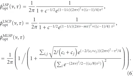
The optimal ambiguity domain kernel in the mean square error sense for zero-mean Gaussian processes was estimated in [4], and based on this, the corresponding kernels for the processes defined in (1), (2), and (3) were derived in [5] as
φLSPopt(ν,τ)=
1 2π
1
1 +c−1/2e(1−1/c)(2πν)2+((c−1)/4)τ2,
φLSCP
opt (ν,τ)=
1 2π
1
1 +c−1/2e(1−1/c)(2πν−mτ)2+((c−1)/4)τ2,
φMLSPopt (ν,τ)
= 1 2π ⎛ ⎜ ⎜ ⎝1 ⎛ ⎜ ⎜ ⎝1 +
i,j
2/ci+cj
e(−2/(ci+cj))(2πν)2−τ2/4
ie−(2πν)
2/2−((c
i/8)τ2) 2 ⎞ ⎟ ⎟ ⎠ ⎞ ⎟ ⎟ ⎠. (6)
The optimal ambiguity domain kernels corresponding to the covariance functions and processes of Figures 1 and2 are computed and plotted inFigure 3.
Instead of calculating the time-frequency estimate using the ambiguity domain kernel, the calculations can be simpli-fied by using a multitaper spectrogram, [8], where Cohen’s class is written as
WC
t,f
=
Ax(ν,τ)φopt(ν,τ)e−i2π(τ f−tν)dτ dν
=
x
u+τ
2
x∗
u−τ
2
ρopt(t−u,τ)e−i2π f τdu dτ.
(7)
Witht=(t1+t2)/2 andτ=t1−t2,
WC
t,f
=
x(t1)x∗(t2)ρopt
t−t1+t2
2 ,t1−t2
e−i2π f(t1−t2)dt
1dt2
=
x(t1)x∗(t2)ρoptrot(t−t1,t−t2)e−i2π f t1ei2π f t2dt1dt2,
(8)
where
ρrot
opt(t1,t2)=ρ
t1+t2
2 ,t1−t2
. (9)
If the kernel ρrot
opt(t1,t2) satisfies the Hermitian property
ρrot
opt(t1,t2)=(ρoptrot(t2,t1))∗, then solving the integral
ρrotopt(t1,t2)q(t1)dt1=λq(t2) (10)
results in eigenvaluesλkand eigenfunctionsqkwhich form a
complete set. The time-lag kernel can be expressed as
ρrot
opt(t1,t2)=
∞
k=1
λkqk(t1)q∗k(t2). (11)
Using the eigenvalues and eigenvectors, (7) is rewritten as a weighted sum of spectrograms,
WC
t,f=
∞
k=1
λk
x(t1)e−i2π f t1q∗k(t−t1)dt1
2. (12)
With just a few λk that differ from zero, the multitaper
spectrogram solution is an effective solution from imple-mentation aspects.
Using discrete-time data, the windows and weights are found from the solution of the corresponding matrix equation
Roptqk=λkqk, k=1,. . .,N, (13)
where the eigenvalues are ordered according toλ1 ≥ λ2 ≥ · · · ≥ λN, and Ropt is the sampled matrix of sizeN×N
corresponding toρrot
opt(t1,t2) in (9) wheret1,t2 = n/Fs,n =
−N/2,. . .,N/2−1. To extract the corresponding samples
of ρrot
opt(t,τ) in an easy way, the time-lag kernel, ρopt(t,τ)
should be sampled with 2Fs, that is, t = n/2Fs, withn =
−N,. . .,N−1 andτ =n/2Fswithn= −2N,. . ., 2N−1 to
cover the required range fort1andt2. The ambiguity domain
kernel φopt(ν,τ) sampled with 2Fs and the discrete fourier
transform (DFT) in the first variable will give the sampled ρopt(t,τ) and the matrix Ropt. Examples of the eigenvalues
and eigenvectors connected to the corresponding matrices Ropt are computed forN = 256 andFs = 7 and depicted
in Figure 4 where the 10 first eigenvalues are plotted in
Figure 4(a) and the three first eigenvectors are seen in Figures
4(b),4(c),4(d), and4(e) for the respective case.
Table1: The mean square error of the LSP-optimal multitapers and weights (LSPopt) compared to optimal choices of parameters of different
methods evaluating the class of LSPs whenc=1.1, 3, and 20.
Method c=1.1 c=3 c=20
LSPopt 19.23 11.85 3.27
WIG 19.27 14.45 7.21
C-W 19.25 (σ=38) 12.67 (σ=1.45) 4.37 (σ=0.15)
HANN 20.80 (Nw=48) 11.97 (Nw=37) 4.39 (Nw=17)
WOSA 25.59 (Nw=44,K=2) 12.69 (Nw=35,K=2) 3.39 (N =25,K=3)
TH MW 25.26 (Nw=54,K=2) 12.51 (Nw=42,K=2) 3.40 (Nw=29,K=3)
PM MW 23.07 (Nw=36,K=2) 11.94 (Nw=30,K=2) 3.46 (Nw=21,K=8)
which was shown to be true in [5]. The eigenvectors for LSP withc = 1.1 and c = 3 have a very similar shape, and it was also shown in [5] that the eigenfunctions approximate Hermite functions and differ with a specific scaling factor. These approximations will be investigated inSection 4.
4. Evaluation
Using the set of windows and weighting factors described in the previous section, a performance comparison of different kernels and multitaper methods is made. For a fair comparison, the optimal parameter values are found for all methods in all evaluations. For the Wigner spectrum (WIG), [20], the time-lag kernel of the Wigner distribution is defined as
ρ(t,τ)=δ(t), (14)
and the Choi-Williams kernel (C-W), [21], has a time-lag kernel defined as
ρ(t,τ)=πσ
|τ|e−π
2σt2/τ2
, (15)
whereσ is optimized for the smallest mean square error in each case. In the computer evaluation, the C-W time-lag kernel for the discrete-time case proposed in [22], Chapter 6, page 271, is used. For the single Hanning window (HANN), the window length Nw is optimized in each case. For the
Welch method (WOSA), [23], also a Hanning window is used with an overlap of 50 % between the windows, and the optimal lengthNw, and number of windowsK is found for
each case. In the Thomson multitaper method (TH MW), the lengths Nw of the K multitapers are optimized, and
the relation with the resolution bandwidth determined by B = (K + 3)/Nw in each case, [24]. The peak matched
multiple windows (PM MW), [25], are designed to give low correlations between subspectra when the spectrum of the random process includes peaks, that is, a spectrum corresponding to a process with large dynamics. It has been shown that this method gives a small mean square error for evoked potentials, [26] as well as for estimation of heart rate variability (HRV), [27]. The window lengths Nw as well as
the number of windowsKare optimized for the best result, and the corresponding resolution bandwidth is determined byB = (K+ 3)/Nw, similarly as for TH MW in each case.
The weighting factors are chosen as the eigenvaluesαk =λk,
k=1,. . .,K, as this choice is close to the optimal weighting
factors, [28]. The reason for comparing with these methods is that either they are very frequently used various applications or they are designed to be optimal for a similar type of process.
The total mean square error is defined as
J=
ν
τ
EAx(ν,τ)·γφopt(ν,τ)−E[Ax(ν,τ)]
2
, (16)
where E denotes expected value. Using a sufficiently large value N and an appropriate sampling frequency Fs,
the discrete-time case will produce results close to the continuous-time case. The parameter γ is used to adjust the kernel φopt(ν,τ) to give the smallest possible mean
square error for every method and choice of parameters. The parameter γ is optimized individually for all methods and parameter cases and is found by derivation as
γopt=
ντE[Ax(ν,τ)]2φopt(ν,τ)
ντE
A2
x(ν,τ)
φ2
opt(ν,τ)
. (17)
In the first simulation, the resulting total mean square errors (MSE) of the LSP-optimal multitapers (LSPopt) for
three different processes defined by (1), with the parameter casc=1.1, 3, and 20, ranging from nonstationary to more stationary processes, are calculated forN=256 andFs=7.
The results of the different methods are presented inTable 1. The optimal choice is compared with a number of other methods, also optimized for the smallest error. For C-W, the parameterσ is varied in different ranges:σ = 1–38 for c = 1.1,σ = 0.05–1.9 for c = 3, andσ = 0.01–0.38 for c=20, to find the minimum value in each case. The window lengthsNwthat give the optimum result for HANN, WOSA,
PM MW, and TH MW are varied betweenNw=30 and 140.
For WOSA, TH MW, and PM MW, a different number of
windows ranging fromK=2 to 8 are also tested to find the number of windows that give a minimum error.
The results show that WIG and C-W give a mean square error very close to the optimal error, Jopt = 19.23 when
c = 1.1 and that, out of the spectrogram methods, HANN gives the best result. Forc = 3, WIG as well as the result of C-W are larger than the spectrogram methods where the PM MW gives an error closer to the optimal mean square errorJopt = 11.85. Forc =20, the result of the TH MW is
0 0.05
1 0
−1
ν
−20
0
20
τ
(a)φLSP
opt(ν,τ), c=1.1
0 0.05
0.5 0
−0.5
ν
−10 0
10
τ
(b)φLSP
opt(ν,τ), c=3
0 0.05
2 0
−2
ν
−20
0
20
τ
(c)φLSCP
opt (ν,τ), c=1.1, m=2
0 0.05 0.1
0.2 0
−0.2 −0.4
ν
−20
0
20
τ
(d)φMLSP
opt (ν,τ),c1=1.1,c2=20
Figure3: The mean square error optimal ambiguity domain kernel corresponding to processes with covariance functions inFigure 1for
N=256 andFs=7: (a)φoptLSP:c=1.1, (b)φLSPopt:c=3, (c)φLSCPopt :c=1.1,m=2, and (d)φoptMLSP:c1=1.1,c2=20.
Table2: The mean square error of the LSCP-optimal multitapers and weights (LSCPopt) compared to optimal choices of parameters of
different methods evaluating the class of LSCPs whenc=1.1, 3, and 20, andm=2,d= −2.
Method c=1.1 c=3 c=20
LSCPopt 19.23 11.85 3.27
WIG 19.27 14.45 7.21
C-W 19.33 (σ=950) 13.23 (σ=37.5) 4.88 (σ=0.275)
HANN 25.49 (Nw=24) 13.35 (Nw=24) 4.44 (Nw=17)
WOSA 30.64 (Nw=21,K=2) 15.76 (Nw=21,K=2) 3.81 (Nw=21,K=3)
TH MW 31.34 (Nw=27,K=2) 15.94 (Nw=27,K=2) 3.82 (Nw=25,K=3)
PM MW 26.65 (Nw=20,K=2) 13.76 (Nw=20,K=2) 3.77 (Nw=19,K=8)
the great variation in the properties of the class of LSPs when cchanges. Whencincreases fromc=1.1 to larger values the process varies from being narrow banded to wide banded. This is why WIG gives a closer optimum value forc =1.1, but TH MW gives the MSE closer to the optimal value for c=20. None of the established methods are able to give small errors in all three cases, even if all possible parameters of the methods are optimized.
The next simulation evaluates the performance for an LSCP, (2) and the corresponding optimal windows, (LSCPopt). In this case, we usem = 2 andd = −2 for the
simulation of all three processes using the samec-values as
in the preceding example. The evaluation is done using the same methods with the C-W parameter varied in the range, σ=25–950 forc=1.1,σ=2.5–95 forc=3, andσ=0.025– 0.95 forc = 20. InTable 2, the results show that WIG and the C-W are almost as optimal as LSCPoptforc =1.1. The
optimal value forc =3,Jopt =11.85 is not reached by any
other method. Forc= 20, the optimal result isJopt =3.27
and the three multitaper methods give the closest result. The last simulation with results shown in Table 3 eval-uates the performance for the optimal window and weights of MLSP, (3), and (MLSPopt), using two different processes
−0.1 −0.05 0 0.05 0.1 0.15
λk
0 5 10
k
(a) eigenvalues
−0.2 −0.1 0 0.1 0.2 0.3
−10 0 10
t
(b)q1–3(t),c=1.1
−0.2 −0.1 0 0.1 0.2 0.3
−10 0 10
t
(c)q1–3(t),c=3
−0.2 −0.1 0 0.1 0.2 0.3
−10 0 10
t
(d)q1–3(t),c=1.1,m=2
−0.2 −0.1 0 0.1 0.2 0.3
−10 0 10
t
(e)q1–3(t),c1=1.1,c2=20
Figure4: Optimal eigenvalues and eigenvectors corresponding to the ambiguity domain kernels inFigure 3forN =256 andFs =7: (a)
the 10 largest eigenvalues, (solid line=LSP,c=1.1 and LSCP,c=1.1,m=2,d= −2, dash-dotted line=LSP,c=3, dotted line=MLSP,
c1 =1.1, andc2=20). Optimal eigenvectors: (b)c=1.1; (c)c=3; (d)c=1.1,m=2,d= −2 (real-valued part only); (e)c1=1.1 and
c2=20.
Table3: The mean square error of the MLSP-optimal multitapers and weights (MLSPopt) compared to optimal choices of parameters for
different methods evaluating the class of MLSPs in three cases:c1=1.1,c2=20;c1=2,c2=10;c1=4,c2=8.
Method c1=1.1,c2=20 c1=2,c2=10 c1=4,c2=8
MLSPopt 37.09 36.88 31.72
WIG 48.87 49.75 46.51
C-W 40.91 (σ=1.1) 40.53 (σ=0.8) 36.00 (σ=0.55)
HANN 38.32 (Nw=41) 38.10 (Nw=35) 33.92 (Nw=31)
WOSA 41.45 (Nw=35,K=2) 38.72 (Nw=32,K=2) 32.68 (Nw=32,K=2)
TH MW 41.44 (Nw=41,K=2) 38.33 (Nw=39,K=2) 32.30 (Nw=35,K=2)
PM MW 38.46 (Nw=31,K=2) 37.23 (Nw=29,K=2) 32.34 (Nw=27,K=3)
c1=1.1,c2=20, the second case withc1=2,c2 =10, and
the third case withc1=4,c2=8. For the C-W, the evaluation
is done usingσthat varies fromσ =0.05–1.9 in the first and second case, and fromσ =0.025–0.95 in the third case. It is seen that none of the methods reach the optimal mean square error for this more complicated process. The HANN and the PM MW, however, give small errors comparable to the error of the MLSPoptmultitapers in the first case. In the last case,
all the multitaper methods are able to reach a small mean
square error. The worst results are produced from the WIG and C-W in all three cases.
5. Approximation of Windows Using
Hermite Functions
First eigenvector
−80 −40 −20
−60 0
log
(
ε1
(
Fs
,
c
,
FH
op
t
))
0 10 20 30 40
Fs
(a)
Second eigenvector
−80 −40 −20
−60 0
log
(
ε2
(
Fs
,
c
,
FH
op
t
))
0 10 20 30 40
Fs
(b) 4th eigenvector
−80 −40 −20
−60 0
log
(
ε4
(
Fs
,
c
,
FH
op
t
))
0 10 20 30 40
Fs
c=1.1
c=3
c=10
c=20 (c)
10th eigenvector
−80 −40 −20
−60 0
log
(
ε10
(
Fs
,
c
,
FH
op
t
))
0 10 20 30 40
Fs
c=1.1
c=3
c=10
c=20 (d)
Figure5: The dependence onFsof the errors between the eigenvector optimal to LSP and the corresponding hermite function for different
c-values. The 1st, 2nd, 4th, and 10th eigenvectors are compared. The eigenvector length isN=256.
This approximation is appropriate in the continuous infinite-length case, but in the finite-infinite-length discrete-time case, a set of Hermite functions might be far from the true eigenvectors. How far, depends on the scaling of the matrix Ropt with use of the sampling frequency parameter Fs.
If Fs is very small, the covariance values are large at
the edges of the matrix Ropt and the Hermite functions
certainly are inappropriate as eigenvectors. WithFstoo large,
the larger part of the power of Ropt will be located in
just a few samples in the middle of the matrix, and the eigenvectors will consist of a few values that differ from zero. A proper choice between these extremes should be carefully considered.
Another result from [5] is that the Hermite functions can be dilated, where the dilation factors depend on c according to c1/4/√2. If these results transfer to the
eachc. Thereby, the whole range ofc-values are easily tuned by a new weighting of the set of computed spectrograms. A scaling of the sampling frequency of the optimal kernel and corresponding time-lag matrixRoptis done according to
Fc
s =
F√sc1/4
2 . (18)
Instead of dilating the Hermite functions, the optimal kernel is dilated for different c-values. Using this c-dependent sampling frequency we investigate a set of Hermite functions,
h1(t)=e−t
2/2
,
h2(t)=2te−t
2/2
,
hk(t)=2thk−1(t)−2(k−2)hk−2(t), k=3,. . .,K,
(19)
witht=n/FHforn= −N/2,. . .,N/2−1. The resulting set
of vectors is
hFH
k =
hk
− N
2FH
· · · hk
N 2FH
T
, k=1,. . .,K.
(20)
The square error
εk(Fs,c,FH)=
hFH
k −q
Fc s
k
T
hFH
k −q
Fc s
k
(21)
is computed for all sets of Hermite functions withFHvarying
from 0.1 to 50 with a step of ΔFH = 0.1. The best set
of Hermite functions is chosen as the one where the sum of square errors between the first eigenvector and the first Hermite function is minimized, that is,
FHopt=arg min
FH
ε1(Fs,c,FH). (22)
Thereby, the whole set of optimal Hermite functionshFHopt
k ,
k = 1,. . .,K, is determined for a specificFc
s. However, the
optimal set of Hermite functions found from this criterion does not necessarily have FHopt = Fs. The resulting square
error εk(Fs,c,FHopt) is studied for a number of differentFs
andc-values, where the sampling frequencyFc
s according to
(18) is used for the computation of the optimal kernel and corresponding multitapers. The results are given inFigure 5
forN=256 and inFigure 6forN=32. The logarithm of the different error vectors forc-valuesc=1.1, 3, 10, and 20 are depicted in the same figure as a function ofFsand the results
are presented for the 1st, 2nd, 4th, and 10th eigenvectors. The results inFigure 5forN = 256 show that for the 1st eigenvector, the samplingFsis less sensitive than that of the
10th eigenvector. The range ofFs, where the error is small, is
between 2.5 and 20 for allqFsc
1 where it is just between 4 and
15 forqFsc
10, see Figures5(a)and5(d). However, with a proper
choice ofFs, the Hermite functions approximate the first 10
eigenvectors in an appropriate way forN=256. Within this range, it can also be verified thatFs=FHopt, and thereby the
same set of Hermite functions can be used independently of the value ofc.
Table4: The appropriate range forFs=FHoptfor small errors when
using Hermite functions as multitapers optimal to LSP for different
values ofN.
N 512 256 128 64 32
intervalFs 7–30 4–12 4–6 3–3.5 2–2.5
InFigure 6, the square errorεk(Fs,c,FHopt) is shown for
N=32, where the error is small in the range ofFsbetween 2
and 2.5 with an maximum error of 10−7 (1.5 and 3.4 if we
allow a larger maximum error of 10−5). Also within these
ranges, it can be verified thatFs=FHopt. The error increases
for the 2nd and 4th eigenvectors. The range of the minimum errors is, however, about the same as that of qFsc
1. For q
Fc s 10
the error is much larger independently ofFs(note the larger
scale on theY-axis). This means that for smallN-values, the higher order eigenvectors are not possible to approximate as Hermite functions with a small error. The corresponding ranges forN=512, 128, and 64 have also been studied, and the results are summarized inTable 4.
6. Reduction of the Number of
Averaged Spectrograms
The only variables left to adapt the optimal set of multitapers to a certain process are the eigenvalues. In Figure 7, the eigenvalues for differentcare depicted where the calculations are made forN=512 andFs=15. Note the logarithmicX
-axis. Using other values ofNwith appropriate corresponding Fs will give equal sets of eigenvalues. Changing Fs andN
do not alter the eigenvalues, as N and Fs just change the
sampling and size of the matrix Ropt. This is verified to
be true ifRopt is still sampled in an appropriate way, with
the choice ofFs in the intervals specified inTable 4. From
Figure 7, it is seen how the eigenvalues vary with c, for example, theλ1decreases slowly whereλ2is first negative and
then positive. For large values ofc, several eigenvalues differ from zero where, for example, forc=2 there are just a few eigenvalues that differ from zero.
An important aspect is that a multitaper spectrogram should be calculated with a reasonable number of windows. This is possible if a major part of the eigenvalues is close to zero. Here, four different levels for the eigenvalues to contribute to the final estimate are suggested based on
λδk=
⎧ ⎪ ⎨ ⎪ ⎩
λk if
λk
λ1
≥δ,
0 otherwise,
(23)
whereδ=0 (i.e., all eigenvalues are included),δ=0.01,δ=
First eigenvector
−70 −60 −50 −40 −30 −20 −10 0
log
(
ε1
(
Fs
,
c
,
FH
op
t
))
0 1 2 3 4 5
Fs
(a)
Second eigenvector
−70 −60 −50 −40 −30 −20 −10 0
log
(
ε2
(
Fs
,
c
,
FH
op
t
))
0 1 2 3 4 5
Fs
(b) 4th eigenvector
−70 −60 −50 −40 −30 −20 −10 0
log
(
ε4
(
Fs
,
c
,
FH
op
t
))
0 1 2 3 4 5
Fs
c=1.1
c=3
c=10
c=20 (c)
10th eigenvector
−70 −60 −50 −40 −30 −20 −10 0
log
(
ε10
(
Fs
,
c
,
FH
op
t
))
0 1 2 3 4 5
Fs
c=1.1
c=3
c=10
c=20 (d)
Figure6: The dependence onFsof the errors between the eigenvector optimal to LSP and the corresponding hermite function for different
c-values. The 1st, 2nd, 4th, and 10th eigenvector are compared. The eigenvector length isN=32.
appropriate estimate, varying betweenK=1–5, dash-dotted line.
A set of Hermite functions hFkHopt, k = 1,. . .,K, is easy to compute, and as the set can also be used as corresponding eigenvectors independently of the parameter cthe advantage is even larger. If we, by this approximation of the eigenvectors, avoid solving an eigenvalue problem from a matrix of size N × N, we should also use the advantage that the eigenvalues can be computed once and for all and stored to be utilized independently of the value of N. We use the computed eigenvalues in Figure 7
and name them λstorek . Using this set of windows and
eigenvalues, the mean square errorJMWδ is computed where δ is determining the limit for the number of averages
in the spectrograms according to Figure 8. The result is compared with Jopt. In Table 5, the results using N = 256
and Fs = 7 is shown. It is apparent that the use of the
Hermite functions does not degrade the result, and also that using δ = 0.01 is equally optimal. With fewer windows (largerδ), a small difference in the mean square error can be seen.
In the next example, the window length is much shorter, N = 32 andFs = 2.5. The results are seen inTable 6. For
Eigenvalues
−0.1 −0.05 0 0.05 0.1 0.15
λk
λ1
λ2 λ3
100 101
c
Figure7: Eigenvalues, dependence on the parameterc.
Number of averaged spectrograms
0 5 10 15 20 25
K
0 5 10 15 20 25 30
c
Figure 8: Number of averaged multitaper spectrograms K for
different values ofc; solid line=δ=0.01, dashed line=δ =0.05,
dash-dotted line=δ=0.2.
Table5: Results of the MSE of the LSP for different parameter choices using Hermite functions as windows and a decreasing
number of eigenvalues,N=256 andFs=7.
Method c=1.1 c=3 c=20
Jopt 19.23 11.85 3.27
J0
MW 19.23 11.85 3.27
J0.01
MW 19.23 11.85 3.27
J0.05
MW 19.29 11.87 3.30
J0.2
MW 19.30 11.87 3.31
and the level δ = 0.01 gives the same result as using all windows, (δ=0).
The last example inTable 7shows the result whenN =
32, butFsis now altered to be outside the appropriate range,
toFs=5. This choice ofFsgives a very large error when all
windows are included in the estimate, (δ=0). The reason of
Table6: Results of the MSE of the LSP for different parameter choices using Hermite functions as windows and a decreasing
number of eigenvalues,N =32 andFs=2.5.
Method c=1.1 c=3 c=20
Jopt 19.23 11.85 3.27
J0
MW 19.23 11.86 3.32
J0.01
MW 19.23 11.86 3.32
J0.05
MW 19.23 11.87 3.34
J0.2
MW 19.29 11.87 3.34
Table7: Results of the MSE of the LSP for different parameter choices using Hermite functions as windows and a decreasing
number of eigenvalues,N =32 andFs=5.
Method c=1.1 c=3 c=20
Jopt 19.23 11.85 3.27
J0
MW 37.62 22.79 8.83
J0.01
MW 19.36 11.85 6.41
J0.05
MW 19.23 11.87 3.30
J0.2
MW 19.30 11.87 3.31
course is that the Hermite functions are not at all appropriate to use for larger K, as they are no longer similar to the eigenvectors. Reducing the number of windows, however, δ ≥0.01, gives a mean square error sufficiently close to the trueJopt. This shows that the Hermite functions together with
limiting the number of windows give an appropriate estimate even ifFsis chosen inappropriately.
7. Estimation of Induced Potential Power in
the Electroencephalogram
To show the performance of the proposed method and especially show the possibility to view the multitaper spec-trograms for different model assumptions, that is, different c-values, examples are shown of the electrophysiological correlates of toddlers’ processing of imperative and declar-ative gestures. Neural responses to video clips displaying different types of nonlinguistic communication between two actors are recorded. Results from investigations of language learning, indicate that there may be important developments in this domain in the second half of the second year, [29]. The hypothesis was that if the comprehension of declarative, but not imperative, communication acts is specific to humans, the processing of these two types of acts should be associated with different neural activity. There is not much research on what young children understand as onlookers of communication between other people. It is important to find suitable models for the time-varying power estimation of these signals.
2 4 6 8 10
Fre
q
u
en
cy
(H
z)
0 1
Time (s) Sub.1, PDec
(a)
2 4 6 8 10
Fre
q
u
en
cy
(H
z)
0 1
Time (s) Sub.1, PImp
(b)
2 4 6 8 10
Fre
q
u
en
cy
(H
z)
0 1
Time (s) Sub.1, PPlay
(c)
2 4 6 8 10
Fre
q
u
en
cy
(H
z)
0 1
Time (s) Sub.2, PDec
(d)
2 4 6 8 10
Fre
q
u
en
cy
(H
z)
0 1
Time (s) Sub.2, PImp
(e)
2 4 6 8 10
Fre
q
u
en
cy
(H
z)
0 1
Time (s) Sub.2, PPlay
(f)
Figure9: Multitaper spectrogram estimation of induced potentials from Protodeclarative (PDec), Protoimperative (PImp) and neutral
parallel play (PPlay) shows, usingN =256,Fs=12,c=1.1, andδ=0.05. The number of averaged power responses are for subject 1, 20
and for subject 2, 29.
the international 10–20 system. The vertical electrooculo-gram (VEOG) was recorded from electrodes placed above and below the right eye, and the horizontal electrooculogram (HEOG) was recorded from electrodes placed lateral to the left and the right eye. All electrodes were referenced to the average of the left and the right mastoids. Impedances were kept below 5 kΩ for all electrodes. The EEG was recorded with a 0.1/70 Hz band-pass filter at a sampling rate of 500 Hz, and amplified with a Neuroscan NuAmps amplifier. The sampling frequency is reduced to 62.5 Hz by decimation in Matlab and before and after the 2s epochs, zeros are added to allow for the total data window length. The included data epochs are limited so that the same number of epochs is used for the declarative, imperative, and parallel play acts. For subject 1, the number of epochs were 20 in each of the three cases, and for subject 2, the number of epochs were 29. The averaged power from two different subjects is estimated using a set of Hermite functions with N = 256 andFs = FHopt = 12. Different sets of eigenvalues are used
as weighting factors, corresponding to c = 1.1, c = 3,
and c = 20. Using δ = 0.05, the estimation of the spectrogram is then done using a reasonable number of
averaged spectrograms, K = 10, K = 2 and, K = 6,
respectively. Remember, that with this procedure only the averaging of the spectrograms need to be redone for a new value of the parameterc, the individual single-window periodograms with the set of chosen Hermite functions are the same. The results of two subjects are shown in Figures
2 4 6 8 10
Fre
q
u
en
cy
(H
z)
0 1
Time (s) Sub.1, PDec
(a)
2 4 6 8 10
Fre
q
u
en
cy
(H
z)
0 1
Time (s) Sub.1, PIpm
(b)
2 4 6 8 10
Fre
q
u
en
cy
(H
z)
0 1
Time (s) Sub.1, PPlay
(c)
2 4 6 8 10
Fre
q
u
en
cy
(H
z)
0 1
Time (s) Sub.2, PDec
(d)
2 4 6 8 10
Fre
q
u
en
cy
(H
z)
0 1
Time (s) Sub.2, PImp
(e)
2 4 6 8 10
Fre
q
u
en
cy
(H
z)
0 1
Time (s) Sub.2, PPlay
(f)
Figure10: Multitaper spectrogram estimation of induced potentials from Protodeclarative (PDec), Protoimperative (PImp) and neutral
parallel play (PPlay) shows, usingN=256,Fs=12,c=3, andδ=0.05. The number of averaged power responses are for subject 1, 20 and
for subject 2, 29.
estimator, (c=20) inFigure 11. This shows the possibility to easily investigate a whole range of estimators when the data model is not well defined.
8. Conclusions
The mean square error optimal multitaper spectrogram estimator, for a class of locally stationary processes is evaluated and compared to other frequently used methods: the Wigner distribution, the Choi-Williams distribution, the single Hanning spectrogram, the Welch method, the Thomson multitapers, and the peak matched multitapers. The results show that it is possible to find other methods that give a result more or less close to the result of the optimal multitapers in mean square error sense, but it is different methods for different processes of the class. An evaluation is also made for the classes of locally stationary chirp processes and sum of locally stationary processes.
An investigation of the error shows that with a proper sampling frequency of the windows, the windows are well approximated by a set of Hermite functions where the same set of functions is valid for the whole class if an appropriate dilation factor is used. Another advantage is that the optimal set of weighting factors can be stored and utilized for all different window lengths. It is also investigated if the number of included spectrograms in the average can be reduced, and the results show that only a small number of windows, 1– 10, are needed for an appropriate approximation of the true kernel.
2 4 6 8 10
Fre
q
u
en
cy
(H
z)
0 1
Time (s) Sub.1, PDec
(a)
2 4 6 8 10
Fre
q
u
en
cy
(H
z)
0 1
Time (s) Sub.1, PIpm
(b)
2 4 6 8 10
Fre
q
u
en
cy
(H
z)
0 1
Time (s) Sub.1, PPlay
(c)
2 4 6 8 10
Fre
q
u
en
cy
(H
z)
0 1
Time (s) Sub.2, PDec
(d)
2 4 6 8 10
Fre
q
u
en
cy
(H
z)
0 1
Time (s) Sub.2, PImp
(e)
2 4 6 8 10
Fre
q
u
en
cy
(H
z)
0 1
Time (s) Sub.2, PPlay
(f)
Figure11: Multitaper spectrogram estimation of induced potentials from Protodeclarative (PDec), Protoimperative (PImp) and Neutral
Parallel Play (PPlay) shows, usingN=256,Fs=12,c=20 andδ=0.05. The number of averaged power responses are for subject 1, 20 and
for subject 2, 29.
processing of imperative and declarative gestures, are shown as example of the use of the proposed method.
Acknowledgments
The author wishes to thank the Swedish Research Council for financing, and she also thanks Associate Professor Mag-nus Lindgren, Department of Psychology, Lund University, Sweden, and Ph.D. Janne von Koss Torkildsen, Department of Biological and Medical Psychology, University of Bergen, Norway, for permission to use experimental data.
References
[1] R. A. Silverman, “Locally stationary random processes,”IRE
Transactions on Information Theory, vol. 3, pp. 182–187, 1957. [2] M. Hansson-Sandsten and J. Sandberg, “Optimization of weighting factors for multiple window spectrogram of
event-related potentials,”EURASIP Journal on Advances in Signal
Processing, vol. 2010, Article ID 391798, 10 pages, 2010.
[3] M. Hansson-Sandsten, “Evaluation of the optimal lengths and number of multiple windows for spectrogram estimation of
SSVEP,”Medical Engineering and Physics, vol. 32, no. 4, pp.
372–383, 2010.
[4] A. M. Sayeed and D. L. Jones, “Optimal kernels for
non-stationary spectral estimation,”IEEE Transactions on Signal
Processing, vol. 43, no. 2, pp. 478–491, 1995.
[5] P. Wahlberg and M. Hansson, “Kernels and multiple windows for estimation of the Wigner-Ville spectrum of Gaussian
locally stationary processes,” IEEE Transactions on Signal
Processing, vol. 55, no. 1, pp. 73–84, 2007.
[6] G. S. Cunnigham and W. J. Williams, “Kernel decomposition
of time-frequency distributions,”IEEE Transactions on Signal
Processing, vol. 42, no. 6, pp. 1425–1442, 1994.
[7] M. G. Amin, “Spectral decomposition of time-frequency
distribution kernels,”IEEE Transactions on Signal Processing,
vol. 42, no. 5, pp. 1156–1165, 1994.
[8] L. Cohen,Time-Frequency Analysis, Prentice-Hall, New York,
NY, USA, 1995.
[9] F. Cakrak and P. J. Loughlin, “Multiple window time-varying
spectral analysis,”IEEE Transactions on Signal Processing, vol.
[10] L. L. Scharf and B. Friedlander, “Toeplitz and Hankel kernels for estimating time-varying spectra of discrete-time random
processes,”IEEE Transactions on Signal Processing, vol. 49, no.
1, pp. 179–189, 2001.
[11] M. Bayram and R. G. Baraniuk, “Multiple window
time-frequency analysis,” inProceedings of the IEEE-SP International
Symposium on Time-Frequency and Time-Scale Analysis, pp. 511–514, June 1996.
[12] S. Aviyente and W. J. Williams, “A centrosymmetric kernel decomposition for time-frequency distribution computation,”
IEEE Transactions on Signal Processing, vol. 52, no. 6, pp. 1574– 1584, 2004.
[13] S. Aviyente and W. J. Williams, “Multitaper marginal
time-frequency distributions,”Signal Processing, vol. 86, no. 2, pp.
279–295, 2006.
[14] M. Hansson, “Multiple window decomposition of time-frequency kernels using a penalty function for suppressed
sidelobes,” inProceedings of the IEEE International Conference
on Acoustics, Speech and Signal Processing (ICASSP ’06), vol. 3, pp. 432–435, Toulouse, France, May 2006.
[15] M. Hansson-Sandsten, “Multi taper wigner distribution with predetermined doppler-lag bandwdith and sidelobe
sup-pression,” in Proceedings of the European Signal Processing
Conference (EUSIPCO ’10), Aalborg, Denmark, 2010. [16] M. S. Richman, T. W. Parks, and R. G. Shenoy, “Discrete-time,
discrete-frequency, time-frequency analysis,” IEEE
Transac-tions on Signal Processing, vol. 46, no. 6, pp. 1517–1527, 1998. [17] A. H. Costa and G. Faye Boudreaux-Bartels, “An overview
of aliasing errors in discrete-time formulations of
time-frequency representations,”IEEE Transactions on Signal
Pro-cessing, vol. 47, no. 5, pp. 1463–1474, 1999.
[18] J. Sandberg and M. Hansson-Sandsten, “A comparison
between different discrete ambiguity domain definitions in
stochastic time-frequency analysis,” IEEE Transactions on
Signal Processing, vol. 57, no. 3, pp. 868–877, 2009.
[19] C. Richard, “Time-frequency-based detection using
discrete-time discrete-frequency Wigner distributions,”IEEE
Transac-tions on Signal Processing, vol. 50, no. 9, pp. 2170–2176, 2002. [20] E. Wigner, “On the quantum correction for thermodynamic
equilibrium,” Physical Review, vol. 40, no. 5, pp. 749–759,
1932.
[21] H. I. Choi and W. J. Williams, “Improved time-frequency representation of multicomponent signals using exponential
kernels,”IEEE Transactions on Acoustics, Speech, and Signal
Processing, vol. 37, no. 6, pp. 862–871, 1989.
[22] B. Boashash, Ed.,Time Frequency Signal Analysis and
Process-ing, Elsevier, New York, NY, USA, 1st edition, 2003.
[23] P. D. Welch, “The use of fast fourier transform for the estima-tion of power spectra: a method based on time averaging over
short, modified periodograms,”IEEE Transactions on Audio
Electroacoustics, vol. 15, no. 2, pp. 70–73, 1967.
[24] D. J. Thomson, “Spectrum estimation and harmonic analysis,”
Proceedings of the IEEE, vol. 70, no. 9, pp. 1055–1096, 1982. [25] M. Hansson and G. Salomonsson, “A multiple window
method for estimation of peaked spectra,”IEEE Transactions
on Signal Processing, vol. 45, no. 3, pp. 778–781, 1997. [26] M. Hansson and M. Lindgren, “Multiple-window
spectro-gram of peaks due to transients in the electroencephalospectro-gram,”
IEEE Transactions on Biomedical Engineering, vol. 48, no. 3, pp. 284–293, 2001.
[27] M. Hansson-Sandsten and P. J¨onsson, “Multiple window correlation analysis of HRV power and respiratory frequency,”
IEEE Transactions on Biomedical Engineering, vol. 54, no. 10, pp. 1770–1779, 2007.
[28] M. Hansson, “Optimized weighted averaging of peak matched
multiple window spectrum estimates,”IEEE Transactions on
Signal Processing, vol. 47, no. 4, pp. 1141–1146, 1999. [29] J. v. K. Torkildsen, H. Friis Hansen, J. M. Svangstu et al., “Brain
dynamics of word familiarization in 20-month-olds: effects of
productive vocabulary size,”Brain and Language, vol. 108, no.