On Sequential Track Extraction within the PMHT Framework

Volume 2008, Article ID 276914,13pages doi:10.1155/2008/276914

Research Article

On Sequential Track Extraction within the PMHT Framework

Monika Wieneke and Wolfgang Koch

FGAN-FKIE, Neuenahrer Strasse 20, 53343 Wachtberg, Germany

Correspondence should be addressed to Monika Wieneke,[email protected]

Received 1 April 2007; Revised 17 August 2007; Accepted 8 October 2007

Recommended by T. Luginbuhl

Tracking multiple targets in a cluttered environment is a challenging task. Probabilistic multiple hypothesis tracking (PMHT) is an efficient approach for dealing with it. Essentially PMHT is based on expectation-maximization for handling with association conflicts. Linearity in the number of targets and measurements is the main motivation for a further development and extension of this methodology. In particular, the problem of track extraction and deletion is apparently not yet satisfactorily solved within this framework. A sequential likelihood-ratio (LR) test for track extraction has been developed and integrated into the framework of traditional Bayesian multiple hypothesis tracking by G¨unter van Keuk in 1998. As PMHT is a multiscan approach as well, it also has the potential for track extraction. In this paper, an analogous integration of a sequential LR test into the PMHT framework is proposed. We present an LR formula for track extraction and deletion using the PMHT update formulae. The LR is thus a by-product of the PMHT iteration process, as PMHT provides all required ingredients for a sequential LR calculation. Therefore, the resulting update formula for the sequential LR test affords the development of track-before-detect algorithms for PMHT. The approach is illustrated by a simple example.

Copyright © 2008 M. Wieneke and W. Koch. This is an open access article distributed under the Creative Commons Attribution License, which permits unrestricted use, distribution, and reproduction in any medium, provided the original work is properly cited.

1. INTRODUCTION

The problem of tracking multiple targets in a realistic en-vironment has been an object of research for a long time. The traditionalapproaches to multiple hypothesis tracking (MHT) rely on the complete enumeration of all possible associationinterpretations of a series of measurements [1]. These Bayesian MHT algorithms use a hard association model which (in the case of point targets) realistically im-plies that a target can produce at most one measurement at a time. A consistent realization of this model would yield an optimal tracking. Unfortunately, as the underlying problem is NP-hard, the resulting hypothesis trees grow exponentially. The so-called growing memory disaster of MHT is avoided by pruning, gating, and combining techniques which lead to an approximation of an optimal tracking. The aim is to dras-tically limit the number of hypotheses by retaining only the most likely ones, while the main risk is to eliminate correct measurement sequences. As a path in a hypothesis tree spans all time scans, from the past up to the present, Bayesian MHT is counted among the multiscan approaches. Another tradi-tional approach is realized by the joint probabilistic data as-sociation filter (JPDAF) [2] that processes only the current

time scan (single scan). The JPDAF is an extension of the simple PDAF for the case of multiple targets. At each scan, JPDAF combines all possible hypotheses to one synthetic hy-pothesis (global combining). The PDAF and JPDAF, respec-tively, are a second-order approximation of an optimal track-ing.

smoother (M-Step), which leads to improved state estimates. The new state estimates flow into the E-Step of the following iteration such that the former association weights can be cor-rected. For each target the E-Step and M-Step are iteratively repeated until the state estimates converge. After shifting the window the iteration process is started for the new window position. The convergence to a local maximum is guaranteed, because this property has been proven for the EM method in general. As PMHT is based on EM, its association model is soft which implies that a target can cause more than one measurement per scan. Of course a soft association model does not reflect the reality if point targets are to be tracked, but it facilitates efficient tracking algorithms. Assuming a soft association model PMHT works optimally, because the EM-Method works optimally in general.

So PMHT is a multiple target tracking algorithm of con-siderable theoretical elegance. Its memory wastage is linear in all parameters: window length, number of measurements, and number of targets. Working on a sliding data window, PMHT takes the information of previous and following time scans into account. Hence, as it is a multiscan approach, it has the potential for track extraction.

Unfortunately, the standard PMHT is limited to the as-sumption that the number of targets is constant and known in advance. Although there exist several approaches for track extraction and deletion within PMHT, this problem is ap-parently not yet satisfactorily solved. The most important task within a track management system is the choice of an appropriate test function for track candidates [7,8]. Some authors [9] use statistical hypothesis testingoutsidePMHT to determine whether a track is true or false. Target visibil-ity is an approach published in [7,10,11]. For track extrac-tion in Bayesian MHT, a sequential likelihood-ratio (LR) test has been proposed in [12]. As this LR test has been success-fully embedded into the framework of Bayesian MHT, we are motivated to try an analogous integration into the PMHT framework. In this work, we derive an LR formula for se-quential track extraction by PMHT. Using this formula the LR is a by-product of the iteration process on the PMHT data window.

The remainder of this work is organized as follows. In Section 2, we provide some basics. The section begins with an introduction of our notations. Afterwards we briefly ex-plain the method of EM and a modification of the PMHT al-gorithm as it is used in our work. InSection 3, we start with the principle of LR testing, as it is proposed in [12]. Then we show the derivation of an LR formula for PMHT.Section 4 presents values of the formula in an experimental example. The last section provides conclusions.

2. PROBABILISTIC MULTIPLE HYPOTHESIS TRACKING

To introduce our notations we start with a formal description of the considered scenario and the task of tracking multiple targets.

Our tracking scenario is defined as follows. A sensor ob-servesSpoint targets in its field of view (FoV). We denote the area of the FoV as|FoV|. The sensor generates measure-mentsZ = Z1:T = {zt,Nt}Tt=1 for a time interval [1 : T].

The sensor output at a scantconsists of not only the set of measurementsztbut also the number of measurementsNt. Thus we model measured data as a pair{zt,Nt}. Measure-mentsznt ∈R2withn∈[1 :Nt] are assumed to be Cartesian position data. The spurious, noninformative measurement

n=0 denotes a missing detection. We introduce it to avoid the hospitality problem of the standard PMHT. Its impact is explained inSection 2.3.

The task of tracking consists in estimating the kinematic statesX=X1:T of the observed targets. The statesxs

t ∈R4 with s ∈ [1 : S] comprise position and velocity. Diffi cul-ties arise from unkown associationsA = A1:T = {at}Tt=1 of measurements to targets. We model the associations as random variablesat = {ant}Nn=t0that map each measurement

n ∈ [0 : Nt] to one of the targetss ∈ [0 : S] by assigning

an

t =s. The targets=0 is a spurious planar target that repre-sents clutter. It corresponds to|FoV|and has been integrated into PMHT by [13]. So mathematically expressed, the opti-mization problem

arg max

X p(X|Z) (1)

is to be solved. Expectation-maximization (EM) is an effi -cient method for this task.

2.1. Expectation-maximization

Expectation-maximization (EM) is an iterative method for localizing posterior modes. It has been derived and explained in many different ways. We decided to follow the work by Dellaert [5], which is one of the more descriptive derivations. At each iteration, EM first calculates posterior weight

p(A|Z,Xl_{). The posterior weights define an optimal lower} bound

QX;Xl_=logp(X)+ A

logp(A,Z|X)pA|Z,Xl

(2)

ofp(X|Z) at the current guessXl_{.lis the iteration index.} AsQ(X;Xl_{) is expressed as an expectation, this first step is} called E-Step. In the following M-Step, EM maximizes the bound with respect to the free variableX, which leads to im-proved estimatesX(l+1)_{. They control the lower bound of the} following E-Step. E-Step and M-Step are repeated until the estimates converge. How the M-Step is done depends on the application. PMHT is the application of EM to the tracking problem. It results in estimatesxtsfor each targets∈[1 :S] at each timet ∈[1 :T]. Covariance matricesPs

t occur as a by-product. They cannot be proven to be the error covari-ance matrices of the point estimatesxs

t, but nevertheless have a useful role.

2.2. Calculating the posterior weights (E-Step)

measurements per target, the random variablesant of the as-sociations are stochastically independent. So applying Bayes’ rule yields

pA|Z,Xl₌ T

t=0 Nt

n=0p

znt |x lan

t

t

pant |Nt

at

Nt

n=0p

znt |xla

n t

t

pant |Nt . (3)

After some technical intermediate steps, that afford an ex-change of product and sum in the denominator of (3), we finally obtain posterior weights

pA|Z,Xl₌ T

t=1 Nt

n=0N

znt;Hxla

n t

t ,Rnt

πnant

t Nt

n=0 Ss=0N

znt;Hxlst,Rnt

πnst

=: T

t=1 Nt

n=0

wlnant

t ,

(4)

withπnst = p(ant = s | Nt). Note that the notation (4) is simplified. With respect to the special casesn=0 ands=0, we point out that the Gaussians are to be understood in an improper sense: as clutter measurements can be assumed to be equally distributed over the FoV, the posterior weight of the clutter targets=0 becomes

wln0 t =σ·

πn0t

|FoV| forn >0,

with normalization constantσ.

(5)

And the intermediate result (3) allows us to assume

wl0a0t

t = π

0a0

t

t S s=0π0st

=π0a0t

t fora0t ∈[0 :S],l∈N0. (6)

As the posterior weights in (4) are governed by the measure-ment covariancesRnt, which is an essential characteristic trait of standard PMHT, they do not take the quality of the cur-rent track estimation into account. This problem of standard PMHT is callednonadaptivityand has already been pointed out by Willett et al. [14]. According to [15] we exchange the measurement covariances by covariancesSlns_:=HPls

tHT+Rnt to make PMHT work adaptively [16]. HereHis the measure-ment matrix andPls

t is the covariance-type matrix being an output of PMHT (seeSection 2.1), which is here interpreted as estimation error covariance ofxlst in the sense of a heuris-tic. This leads to posterior weights

pA|Z,Xl₌ T

t=1 Nt

n=0N

zn t;Hxla

n t

t ,Slna

n t

t

πnant

t Nt

n=0 Ss=0N

znt;Hxlst,Slnst

πnst

=: T

t=1 Nt

n=0

wlnant

t .

(7)

The posterior weights comprise two kinds of measures that evaluate the relevance of a measurement with respect to a target estimation: a distance measure which is given by the GaussianN(znt;Hxlst,Slns) and a visibility measure denoted asπnst . In the case ofn > 0 the latter reflects how likely it

is to hit a target, not taking concrete position data into ac-count. The weightπ0st simply is the probability of missing a target and its impact is explained inSection 2.3. In standard PMHT,πnst =p(ant =s) is the association prior which is esti-mated iteratively by summing up the posterior weights of the current target and dividing this by the number of measure-mentsNt [3]. In [7,10] it is proposed to estimateπnst by an HMM smoother.

We modeled the sensor output as a pair{zt,Nt}. So we can split the pair and treatNt separately. This leads to pos-teriorsπns

t := p(ant = s | Nt), with respect to the number of measurementsNtin the FoV. As already proposed in [14], (Section II.C.: PMHT Implementation Issues, issue 3: Prior Probabilities) and [17], theseweights can becalculatedbefore starting the iteration process and need not to be estimated iteratively. The calculation method is based on a valid sta-tistical sensor model, that is the correct value is conditioned on the number of measurementsNt received in scant, and parameterized by the clutter density, by|FoV|and the prob-ability of detectionPD, which is assumed to be equal for all targets. The idea behind this approach is the following: the original PMHT allowsmorethan one measurement per tar-get in each scan (i.e., in contrast to the physical measure-ment process), the calculation ofπnst is an attempt to make use of the physically “correct” assignment model without de-stroying linearity in the number of targets. We exemplarily show the derivation via Bayes’ rule for the case of n > 0,

s > 0,Nt > 1, and a single target (S = 1). For the prior we simply get p(ant =1)=PD/((1−pF(0)) +PD), whereas the denominator results from the normalization with respect to the targets. pF(0) denotes the probability of having no false measurements (Poisson distributed). Now we are look-ing for the probability of havlook-ing Nt measurements. As at most one of the measurements can be associated with the real target, the remaining measurements must be clutter. So we have p(Nt | ant =1) = pF(Nt−1) and finally come to

p(an

t =s|Nt) via Bayes’ rule. Further details about the cal-culationπnst can be found in [16]. We also derived formulae for the case of detecting the clutter target (πn0t ,n > 0) and missing the real target (π01t ).

In a scenario of multiple targets (S > 1) we use bino-mial coefficients to calculate πnst . Again we show the case

n > 0 ands > 0, that is we are looking for the probabil-ity πnst of detecting the real target. The calculation of the prior is completely analogous to the single target scenario

S = 1. Let us consider p(Nt | ant = s). It is given in ad-vance that a measurementn∈[1 :Nt] refers to a real target

s ∈ [1 : S]. Hence, at least one real target is detected. So we have p(Nt = 0 | ant = s) = 0 because there is at least one measurement.Nt ∈[1 : S] measurements can be gen-erated as follows: one measurement is given by the detection of the real targetan

t =s. To generate the remaining measure-ments we can use anothersD ∈ [0 : Nt−1] detections of real targets. Additionally there are [Nt−1 : 0] false measure-ments to be produced. For the selection of a number ofsD real targets there areSs−D1

one measurement arises from the given detection. Besides, anothersD ∈[0 :S−1] detections of real targets can be in-cluded. Additionally [Nt−1 : Nt−S] false measurements have to be produced:

p(Nt|ant =s)= ⎧ ⎪ ⎪ ⎪ ⎪ ⎪ ⎪ ⎪ ⎪ ⎪ ⎪ ⎪ ⎪ ⎪ ⎪ ⎪ ⎪ ⎨ ⎪ ⎪ ⎪ ⎪ ⎪ ⎪ ⎪ ⎪ ⎪ ⎪ ⎪ ⎪ ⎪ ⎪ ⎪ ⎪ ⎩

0, Nt=0,

Nt−1

sD=0

pF(Nt−sD−1)

S−1

sD

×PsD

D(1−PD)(S−1−sD), Nt∈[1 :S], S−1

sD=0

pF(Nt−sD−1)

S−1

sD

×PsD

D(1−PD)(S−1−sD), Nt> S. (8)

NotesDdoes not contain the target that is already known as detected. In the case ofPD =1 there are at leastS measure-ments. Hence, we have p(Nt | ant = s)=0 forNt < Sand

p(Nt |ant =s)=pF(Nt−S) forNt ≥S. The remaining for-mulae and an extensive discussion can be found in [16]. Note that theπnst have to be normalized with respect to the targets.

2.3. Maximizing theQ-function (M-Step)

Because theQ-function can be rewritten as a sum

Q(X;Xl₎

=

S

s=0

logpxs0

Initialization

+ T

t=1

logNxst;Fxst−1,D

Dynamics model

+ Nt

n=0

logNzn t;Hxst,Rnt

πns t wlns t Sensor model (9)

over the targets, the maximization problem decomposes into

Sindependent problems: one summand per target. Let us de-note one of the summands byQs_(X;Xl_{). Obviously the} re-sult of the maximization is not affected by multiplying the summand by an arbitrary constantαl

s>0 leading to

Qs_X;Xl

=logpx0s

αls Initialization

+ T

t=1

logNxs

t;Fxst−1,D

αl

s Dynamics model

+ Nt

n=0

logNznt;Hxst,Rnt

πnst

wlnst αls

Sensor model, (10)

αl

s > 0 is constant over all scanstof the current data win-dow and all measurementsn. It can be varied with respect to

the targetssand the iteration indexl. After shifting the data window new constantsαl

scan be chosen. The sum over the measurements

Nt

n=0

logNznt;Hxst,Rnt

πnst

wlnst αls

=

Nt

n=0

logNzn

t;Hxst,Rnt

wlns

t αls+ const.n

(11)

contains expressions const.n _{:= logπ}ns

t wnst αlswithn ∈ [0 :

Nt]. As these expressions do not depend onXs_{, they are} irrel-evant for the maximization and can be ignored. Additionally we are allowed to apply the monotonically increasing expo-nential function, which also has no impact on the maximiza-tion result forQs_(X;Xl_{). Then for eachn, the summand in} the right part of (11) becomes

explogNznt;Hxst,Rnt

wlns t αls

=Nznt;Hxst,Rtn wlns

t αls

∝ 1

|2πRnt|

expνns t Rn t −1 wlns t αlsνtns

∝Nzn t;Hxst,

Rnt

wlns t αls

,

(12)

with νtns := znt −Hxst, the innovation of measurementznt. Starting with theQ-function (10), we thus obtain

Nt

n=0

logNzn

t;Hxst,Rnt

πns t

wlns

t αls∝ Nt

n=0 Nzn

t;Hxst, Rnt

wlns t αls

(13)

for the measurement sums (over n). Analogously, with re-spect to the time sum (overt), we have

T

t=1

logNxs

t;Fxst−1,D

αl s ∝

T

t=1 Nxs

t;Fxst−1, D αl s

. (14)

Successively applying the product formula (A.3) to expres-sion (13), finally yields relation (15) with evolution matrixF and process noise covarianceD. ¯zlst and ¯Rlst denote synthetic measurements and corresponding error covariances, respec-tively:

expQs(Xs0:T;Xls0:T)

∝p(xs0)α

l s

T

t=1

Nxst;Fxst−1, D αl s

N¯zlst;Hxst, ¯Rlst

(15)

with

¯ zlst =R¯lst

Nt

n=0

wtlnsαls(Rnt)−1znt, R¯lst = Nt

n=0

wlnst αls(Rnt)−1 −1

.

(16)

αl

weighted sum of measurements. Hence, as it is also contained in ¯Rlst, it can be canceled down.

Considering the standard PMHT in a Cartesian system, that is, the caseαl

s =1 without taking the measurement of the typen=0 into account and withRconstant for all mea-surements, one obtains centroid measurements

¯ zls

t = Nt

n=1wlnst znt Nt

n=1wtlns

with covariances ¯Rls t =

R Nt

n=1wtlns

.

(17)

As already pointed out in [14], the standard PMHT suf-fers from the so-calledhospitalityproblem: the association weights wlns

t are normalized with respect to the targets. Hence, summing them up over the measurements could re-sult in a value greater than unity, which makes the synthetic measurement covariance smaller thanR. As a consequence, the standard PMHT welcomes multiple measurements as only one measurement of high accuracy.

To avoid the hospitality effect, we choose αl

s := 1/ ( NT

n=0wTlns) and make use of the measurement n = 0 rep-resenting a missing detection as follows: Because the “mea-surement” covariance for n = 0 is infinitively great, it is (R0

t) −1

≈0, and the corresponding summands in (16) van-ish. So in a Cartesian system, that is, with R constant for all measurements, we finally obtain centroid measurements with covariances

¯ Rls

t = R αl

s Nn=t1wtlns , αl

s NT

n=1

wlns T =

NT

n=1

wlnsT NT

n=0wlnsT

<1.

(18)

This has an intuitive interpretation: at the latest scanTof the data window, the choice ofαl

sleads to a renormalization of the assignment weightswTlns. It enforces the sum in the de-nominator of (18) to be less than unity and hence mitigates the hospitality problem at the head of the data window. The posterior weightwTl0sis given byπ0sT (seeSection 2.2), which is the probability of missing the target. Note that the integra-tion ofαl

sonly has an impact on the synthetic measurement covariances ¯Rlst and not on the synthetic measurements ¯zlst. It must be pointed out that for elapsed scanst=1,. . .,T−1, this choice ofαl

sdoes not lead to a renormalization with re-spect to the measurements and that at these scans the hos-pitalityproblem is possible and can even be increased. But in the pasthospitalityeffects have a good chance to be cor-rected by the Kalman retrodiction (Rauch-Tung-Striebel re-cursion). The most sensitive PMHT estimation is at the head of the data window, where our approach avoidshospitality.

The above considerations make clear that the PMHT method of estimatingXs_{for each target is invariant under} the replacementRnt→Rnt/αlsandD→D/αls. The arbitrary con-stantαl

sis therefore an internal degree of freedom inherent to PMHT. The standard formulation assumesαl

s=1, for all

s,l. However, any other choice is legitimate, which affords a multitude of PMHT variants.

Now let us return to the formulation of the PMHT al-gorithm. The expression (15) is maximized by an ordinary

Kalman smootherthat processes the synthetic values. As a re-sult we get improved state estimates that flow into the follow-ing E-Step. So for each target, the data of the current PMHT window is processed as follows.

(1) Expectation-step: calculation of posterior weightwtlns

The weights are calculated for all scans of the current win-dow position. They are based on the measurementszn

t and the state estimationsxls

t. Afterwards these weights are used to calculate the synthetic measurement ¯zlst and corresponding error covariances ¯Rlst.

(2) Maximization-step: application of a Kalman smoother

Using the synthetic values of the E-Step, a Kalman filter is applied to the data window. The following retrodiction yields new, improved estimationx(l+1)s0:T .

After convergence, the predictionx_T+1s _|T is to be calcu-lated for the following window position. When all targets have been processed, the window is shifted by one scan.

3. SEQUENTIAL TRACK EXTRACTION BY PMHT

We need a technique that extracts the tracks of an unknown number of targets in the FoV. This should happen as fast as possible and as reliably as requested. Compared with the state estimation in track maintenance, the required algo-rithm works on a higher level of abstraction, that is, we are not looking for single target states but for whole tracks. A sequential likelihood-ratio (LR) test is a technique that ana-lyzes the inflowing measurements with this objective.

3.1. Likelihood ratio testing

In [12] a sequential LR test has been integrated into the Bayesian MHT of well separated targets. Thereby the extrac-tion of a track is modeled as a decision between two com-peting hypothesesH0andH1. Referring to the given series of measurementsZ1:t, they have the following meanings:

H1: the seriesZ1:tcontains data from the target and possi-bly clutter;

H0: no target exists, hence all data inZ1:tare false. The aim is to decide as fast as possible and as reliably as re-quested betweenH1andH0. A sequential LR test consists in successively updating the ratio LR1(t) (19) between the two likelihood functionsp(H1|Z1:t) andp(H0|Z1:t):

LR1(t)=

p(Z1:t|H1)

p(Z1:t|H0)=

p(zt|Z1:t−1,H1)

p(zt|Z1:t−1,H0)·LR(t−1). (19)

At each scantthe value LR1(t) is compared with two thresh-oldsAandB.

(i) If LR1(t)≤A, hypothesisH0is accepted to be true. (ii) If LR1(t)≥B, hypothesisH1is accepted to be true. (iii) Otherwise the algorithm cannot come to a decision yet

This general scheme was first proposed by Wald [18]. The user has to preset the reliability of the algorithm by deter-mining the thresholdsAandB. Thereto they have to set the related statistical decision errorsP1 :=Prob(acceptH1|H1) andP0 :=Prob(acceptH1 | H0). P1 is the probability to rightly identify a really existing target as a target, whereasP0 is the probability to wrongly assume the existence of a target that does not exist. The thresholdsAandBdepend on the errorsP1andP0as follows:

A≈1−P1

1−P0, B≈

P1

P0. (20)

The smaller the permitted error, the longer the user has to wait for the decision. For example, ifP1is chosen near unity andP0is chosen near zero (corresponding to a certainty near 100%), the runtime would by infinitively long. If the deci-sion is requested immediately, all possible combinations of measurements will be identified as targets.

The main result of [12] is the derivation of LR1(t) as a sum over the (not normalized) weights of all possible inter-pretations ofZ1:t. An interpretation corresponds to a path from the root to a leaf of the hypothesis tree. This allows a seamless transition into the phase of track maintenance.

3.2. Likelihood-ratio calculation by PMHT

As the LR test has been successfully embedded into the framework of Bayesian MHT, we are motivated to integrate it into PMHT in an analogous manner. Like Bayesian MHT, the PMHT counts among the multiscan approaches and hence complies with the requirements of such an integration. This section shows how the LR is calculated by PMHT as a by-product.

The following derivation relies on the assumption, that eitherStargets reside in the FoV or none. Accordingly we define hypothesesHSandH0as follows:

HS: the seriesZ1:tcontains data fromStargets and possibly clutter;

H0: no targets exist, hence all data inZ1:tare false. Assumption: HSandH0exclude each other.

As the sensor output is modeled as a pair{zt,Nt}, we can split it and treatNtseparately. So (19) leads to the following equation:

LRS(t)= p

Z1:t|HS

pZ1:t|H0 = p

zt|Nt,Z1:t−1,HS

pzt|Nt,Z1:t−1,H0

F1

·p

Nt|HS

pNt|H0

F2

·p

Z1:t−1|HS

pZ1:t−1|H0 .

(21)

The key idea on adopting van Keuk’s sequential LR test is a new formulation of the hypothesesHSandH0. That is, in fac-torF1of (21),HSandH0are defined by using the detection probabilityPDas follows:

HS≡HS∧(PD0),

H0≡HS∧(PD≈0).

(22)

The decision betweenSand zero targets is now completely controlled byPD (assumed to be equal for all targets). The probabilities in factorF2of (21) can be easily calculated. The numerator can be written as

pNt|HS

=

s

pNt|ant =s

with

n∈0 :Nt

arbitrary, but fixed.

(23)

The summandsp(Nt |ant =s) are the visibility weights that have been introduced and briefly explained in Section 2.2. The denominator represents the probability of having Nt false measurements at scan t, which can be modeled by a Poisson distribution. We denote it as pF(Nt). So we finally get

LRS(t)= p

zt|Nt,Z1:t−1,HS,PD0

pzt|Nt,Z1:t−1,HS,PD ≈0

·p

Nt|HS

pF

Nt

·LRS(t−1).

(24)

The PMHT algorithm works on the basis of synthetic mea-surements. Letlbe the number of the current PMHT itera-tion ands∈[1 :S] one of the targets. At each time stept, the processing of multiple measurementsz0t,. . .,zNttis put down to the processing of a single measurement ¯zlst. Thus in the se-quential LR calculation by PMHT, we follow that principle and consider the ratio between the likelihood functions with synthetic measurements

LRS(t)“=” p(¯zt|Nt,Z1:t−1,HS,PD0)

p(¯zt|Nt,Z1:t−1,HS,PD ≈0)

F1

·p(Nt|HS)

pF(Nt) ·LRS(t−1),

(25)

which is a plausible heuristic approximation of (24). Thereby the vector ¯zt := (¯z1t,. . ., ¯zSt) denotes the synthetic measure-ments of all targets at scantafter thelastiteration (on the window that ends at scant).

In the following, we consider only the numerator ofF1 in (25) and continue by including the target states xt via marginalization (26). Then assuming that target states are stochastically independent, we come to the product:

p¯zt|Nt,Z1:t−1,HS,PD0

=

!

p¯zt,xt|Nt,Z1:t−1,HS,PD0

dxt

(26)

=

S

s=1 !

pz¯s

t,xts|Nt,Z1:t−1,HS,PD0

dxs t. (27)

state of the targetdts≡ detected,¬dst≡ not detected). After marginalization overdtswe get

!

pz¯st,xts|Nt,Z1:t−1,HS

dxst

=! "p¯zs

t,xst,dst|Nt,Z1:t−1,HS

+pz¯st,xst,¬dst|Nt,Z1:t−1,HS #

dxts

=! "p¯zs

t,xst|dts,Nt,Z1:t−1,HS

×pdts|Nt,Z1:t−1,HS

=:πds t

+pz¯s

t,xst| ¬dts,Nt,Z1:t−1,HS

×p¬ds

t|Nt,Z1:t−1,HS

=:π¬ds t

# dxst.

(28)

The termsπds

t andπ¬tds represent the detection probability of a target, given the number of measurementsNt. And they are somewhat similar to the visibility weightsπnst = p(ant =

s| Nt) inSection 2.2. Butπnst is normalized with respect to the targetss ∈[0 : S]. In (28) we consider a fixed targets, that is, one of the factors in (27) and marginalize over the targets detection statedst. Such a marginalization requires a normalization with respect to the measurements, that is, for

n >0 ands >0 we haveπnst,renorm=πnst /(π0st +Nt·πnst ) because

πnst = p(ant =s|Nt) are the same for all real measurements

n∈[1 :Nt] in scant:

π¬ds t =p

¬ds

t|Nt,Z1:t−1,HS

=π0s t,renorm,

πds t =p

ds

t|Nt,Z1:t−1,HS

=Nt·πnst,renorm.

(29)

Furthermore,πdst andπ¬tdsare independent of the integra-tion variablexs

t. Thus

. . .

=πds t

! "

p¯zst|xts,dts,Nt,Z1:t−1,HS

D1

×pxst|dts,Nt,Z1:t−1,HS

D2

# dxts

+π¬ds t

! "

pz¯st|xst,¬dts,Nt,Z1:t−1,HS

D3

×pxst| ¬dts,Nt,Z1:t−1,HS

D4

# dxst.

(30)

The probabilitiesD1andD2refer to the case of detecting the targets.D1is the likelihood functionp(¯zst |xst,dst,HS) ofxst. It is assumed to be Gaussian:N(¯zst;Hxts, ¯Rst). InD2the state xtsis dependent of the measurementsZ1:t−1of elapsed scans. So for the current scant, the whole information of measure-ments is contained in the predictionx_ts_|t−1. As for the cur-rent scan the measuring information is not given, the vari-ablesdtsandNthave no impact. So it makes sense to model

p(xst|Z1:t−1,HS) as a GaussianN(xst;xts|t−1,Pst|t−1) (see (31)

1.2 ×104 1 0.8 0.6 0.4 0.2 0 −0.2 −0.4 −0.6 −0.8 −1 −4000 −2000 0 2000 4000 6000 8000 10000 12000 14000

17 17

16 15 14 15

13 13

12 12 11

9 10 5 8

8 7

10 5

8 4

3 ₄ Missed

Sensor

Missed

Figure1: Movement of an aircraft along a straight line.

1st summand). The probabilitiesD3andD4refer to the case of missing the target. If the target has not been detected,D3is not constant. On every unit of the area|FoV|, ¯zs

tcan be found with equal probabilityp(¯zs

t|xst,¬dst,HS)=1/|FoV|.D4stays below the integral and vanishes because of the normalization property (31), 2nd summand).

Using the product formula (A.1), (31) can be trans-formed into (32):

!

pz¯st,xts|Nt,Z1:t−1,HS

dxst

= · · ·

=πdst ! $

Nz¯st;Hxst, ¯Rst

Nxst;xts|t−1,Pst|t−1 %

dxst

+π¬tds 1

|FoV| !

pxst|. . .

dxst

(31)

=πdst N

¯

zst;Hxst|t−1,HPst|t−1H+ ¯Rst

=:¯Ss t

!

Nxst;. . .

dxts

+π¬ds t

1

|FoV|.

(32)

Thereby ¯Sst is the synthetic innovation covariance after the last PMHT iteration. Inserting (32) into (27) yields the fol-lowing expression for factorF1of (25):

p¯zt|Nt,Z1:t−1,HS,PD0

p¯zt|Nt,Z1:t−1,HS,PD≈0

=

S

s=1

πdst N

¯

zst;Hxst|t−1, ¯Sst

+π¬tds(1/|FoV|)

πdst,PD≈0

≈0

N¯zst;Hxts|t−1, ¯Sst

+π ¬t,PdsD≈0

≈1

(1/|FoV|).

7000 6500 6000 5500 5000 4500 4000 1000 1500 2000 2500 3000 3500 4000

4

6

5₅

4 4

t F1·F2 3

4 5

6

7 8 9 10 11 12 13 14 15 16 17 18 19

124307.556 3436.858 4807.037

0.025

(a)

5000 4500 4000 3500 3000 2500 2000 2000

2500 3000 3500 4000 4500 5000

4 8₈

8

8 7 ₇

6

t F1·F2 3

4 5

6

7 8 9 10 11 12 13 14 15 16 17 18 19

124307.556 3436.858 4807.037

0.025

1139.579 2997.305

(b)

Figure2: Missing detection (t=6), aftereffect (t=7), clutter (t=8).

The hypothesisH0is expressed byHS∧(PD ≈0). In the case of no targets we haveπdst ≈0 andπ¬tds≈1. So (33) and (25) yield our final LR formua:

LRS(t)∝

S

s=1

πds t N

¯ zs

t;Hxst|t−1, ¯Sst

·|FoV|+π¬ds t

F1

·p

Nt|HS

pF

Nt

F2

·LRS(t−1).

(34)

Note that all ingredients of our LR formula are provided by PMHT. Thus the LR calculation (34) is a by-product of the PMHT iteration process.

3.3. Extracting a target cluster by PMHT

Sequential LR testing can well be extended to the problem of extracting target clusters with an unknown number of targets involved [12,19]. To this end assume that the numberKof

targets involved in a cluster is limited byKmax(not too large). The ratio of the probabilityp(H1∨H2· · · ∨HK|Z1:t) that a cluster consisting of at least one and at mostKtargets ex-ists, versus the probability of having false returns only, can be written as

pH1∨ · · · ∨HK|Z1:t

pH0|Z1:t

=

K n=1p

Hn|Z1:t

pH0|Z1:t

=

K

n=1

pZ1:t|Hn

pZ1:t|H0 p

Hn

pH0 .

(35)

We thus obtain in a natural way a generalized test function LRK(t) = (1/K) nk=1LRn(t) with LRn(t) =

p(Z1:t|Hn)/ p(Z1:t|H0) to be calculated in analogy to the case

3000 2500 2000 1500 1000 500 0 3000 3500 4000 4500 5000 5500 6000

10 10

9

8 8

8 8

t F1·F2 3

4 5

6

7 8

9

10 11 12 13 14 15 16 17 18 19

124307.556 3436.858 4807.037

0.025

1139.579 2997.305

0.02

276.007

Figure3: Missing detection (t=9).

500 0 −500 −1000 −1500 −2000 −2500 4500 5000 5500 6000 6500 7000 7500

12₁₂

11 11

9 10

t F1·F2 3

4 5

6

7 8

9

10 11 12 13 14 15 16 17 18 19

124307.556 3436.858 4807.037

0.025

1139.579 2997.305

0.02

276.007 4556.095 4497.803

(a)

−2000 −2500 −3000 −3500 −4000 −4500 −5000 6000 6500 7000 7500 8000 8500 9000

14 14

13 13

13 13

12 14

12 12

12

t F1·F2 3

4 5

6

7 8

9

10 11 12 13 14 15 16 17 18 19

124307.556 3436.858 4807.037

0.025

1139.579 2997.305

0.02

276.007 4556.095 4497.803 2354.912 1126.75

(b)

−5000 −5500 −6000 −6500 −7000 −7500 −8000 7500 8000 8500 9000 9500 10000 10500

17 17

17 16

16

15

1515

t F1·F2 3

4 5

6

7 8

9

10 11 12 13 14 15 16 17 18 19

124307.556 3436.858 4807.037

0.025

1139.579 2997.305

0.02

276.007 4556.095 4497.803 2354.912 1126.75 2991.504 3647.314 1806.277

(a)

−7500 −8000 −8500 −9000 −9500 −10000 −10500 0.9 0.95 1 1.05 1.1 1.15 1.2 ×104

19

18

17 17

t F1·F2 3

4 5

6

7 8

9

10 11 12 13 14 15 16 17

18 19

124307.556 3436.858 4807.037

0.025

1139.579 2997.305

0.02

276.007 4556.095 4497.803 2354.912 1126.75 2991.504 3647.314 1806.277

0.019 0.081

(b)

Figure5: Vanishing of the aircraft at scant=17.

targets within the cluster is thus given by ¯n = K n=1nc(n). Using the results ofSection 3.2, (35) can also be evaluated within the PMHT framework.

4. EXPERIMENTAL EXAMPLE

This section shows the values of the productF1·F2during the tracking. We simulated a simple scenario with one target. A rotating radar observes an aircraft in its FoV. The total length of observation is 25 scans. The aircraft moves along a straight line. The movement starts at scan 1 and ends at scan 16. Since scan 17 we generated false measurements only. The distance

Δtbetween two consecutive scans is 5 seconds (time of cir-culation). False measurements are generated with a density

ρF=10−7.2 (in events per m2). For the aircraft we assumed a detection probabilityPD = 0.8.Figure 1shows the mea-surements of scan 3 up to scan 17. The distance labels on the axes refer to meters. The plot shows real measurements as green crosses +, labeled by scan numbers. False alarms are marked as red crosses +. They are plotted only within a

ra-dius of 3000 m around the true position. At the scanst=6 andt=9 the aircraft was not detected.

4.1. Implementation issue

Starting with a window length of 3, we let the PMHT window grow up to a length of 7 scans and shifted it (by one scan) until the head reached scan 25. At each window position 7 EM iterations were processed. In the following figures, we use black color (+) for the predictionxst and its error ellipsoid. The particular synthetic measurement ¯zst is noted as a blue cross×.

From a formalistic point of view, the parameterαl shas to be constant over all scanstof the current data window and all measurementsn. During our experiments we found out that the results could be improved using a time-adaptive param-eterαl

s(t) that varies over the scans inside the data window. Choosingαl

−1 ×104 −1.05

−1.1 −1.15 −1.2 −1.25 −1.3 8000 8500 9000 9500 10000 10500 11000

20

20

18 19

20

19 t₄ F1·F2

5

6

7 8

9

10 11 12 13 14 15 16 17

18 19 20

3436.858 4807.037

0.025

1139.579 2997.305

0.02

276.007 4556.095 4497.803 2354.912 1126.75 2991.504 3647.314 1806.277

0.019 0.081 3.361

(a)

−1.15 ×104 −1.2

−1.25 −1.3 −1.35 −1.4 −1.45 6000 6500 7000 7500 8000 8500 9000

21 18 18

20

21 20

19

t F1·F2 5

6

7 8

9

10 11 12 13 14 15 16 17

18 19 20 21

4807.037

0.025

1139.579 2997.305

0.02

276.007 4556.095 4497.803 2354.912 1126.75 2991.504 3647.314 1806.277

0.019 0.081 3.361 0.114

(b)

Figure6: Scan 20 and 21.

−1.35 ×104 −1.4 −1.45 −1.5 −1.55 −1.6 −1.65 4000 4500 5000 5500 6000 6500 7000

23

22

21

t F1·F2

6

7 8

9

10 11 12 13 14 15 16 17

18 19 20 21 22 23

0.025

1139.579 2997.305

0.02

276.007 4556.095 4497.803 2354.912 1126.75 2991.504 3647.314 1806.277

0.019 0.081 3.361 0.114 0.021 0.439

4.2. Discussion of the example

From scan 3 up to 5 there are neither missing detections nor disturbing impacts by false measurements. The synthetic measurement ¯zst coincides quite well with the measurement that refers to the aircraft. Hence we can observe high values ofF1·F2(Figure 2(a)).

At scan 6, the aircraft was not detected. Hence ¯zst = (5114, 5285)is far away fromxs_t|t−1and has a large measure-ment error: ¯Rst(1, 1)=R¯st(2, 2)=8.8017·1023and ¯Rst(2, 1)=

¯

Rst(1, 2) = −2.1156·1023. According to this, F1·F2 is small (<1).

Because of the missing detection at scant =6, the pre-diction for scan 7 is bad, which is reflected by the blown up error ellipsoid (Figure 2(b)). As a consequence the prediction does not coincide with the synthetic measurement ¯zstas well as it did during the preceding scans, and so the correspond-ing value ofF1·F2is worse. Att=8, the PMHT recovered. But near the measurement of the aircraft, there is a false one. The synthetic measurement is the mean of both. It is farther away from the prediction than the measurement of the air-craft, and represents a different direction of movement. Thus

F1·F2 is smaller, compared with the scanst = 3, 4, 5. This can be an indication for an impending lost of the track, be-cause the estimations iteratively evolve a tendency towards the synthetic measurement. Therefore, the prediction at scan 9 sheers to the left (Figure 3).

At scan 9 the aircraft was again not detected and we ob-serve the same effect as at scan 6:F1·F2 <1. Because of this missing detection in combination with the sheering at scan 8, the prediction for scan 10 is relatively bad. According to this—compared with the other scans the aircraft has been detected at—the value of F1·F2 (276.007) is perspicuously worse.

At the scans 11and 12 the track is again stable. The val-ues ofF1·F2approximately lie at 4500 (Figure 4(a)). And the false measurement at scan 13 again leads to a drift of the es-timation. Therefore, the value ofF1·F2for scan 14 amounts only to 1126.750 (Figure 4(b)). The PMHT again recovers at the scans 15 and 16. In each case, the synthetic measurement coincides with the measurement of the aircraft. And the pre-diction hits this position quite well, as the productF1·F2 re-flects (Figure 5(a)).

At scan 17 the aircraft has not been detected. But a false measurement is picked up, that continues the track in an ex-pedient way. At all further scans, the aircraft is also not de-tected. Its track ends at scan 16 (or at latest 17). According to this,F1·F2is relatively small (<1) (Figures6and7).

At scan 20 the synthetic measurement is (by chance) lo-cated in the further surrounding of the prediction. The con-sequence is a slight increase ofF1·F2to 3.361 (Figure 6).

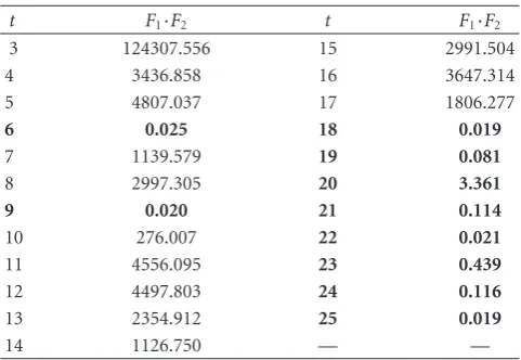
Table 1shows all values ofF1·F2, recapitulating. Follow-ing [12] this value has to be multiplied with the previous LR at each scan (successive update). We see thatF1·F2can be of a relatively high magnitude, which causes a fast increase while successively updating the LR. A possible means to reduce the magnitude could be the use of logarithmic values. But this idea has to be checked quite carefully because the logarithm becomes negative in case of values that are smaller than unity.

Table1: LR calculation for a track of a single target.

t F1·F2 t F1·F2

3 124307.556 15 2991.504

4 3436.858 16 3647.314

5 4807.037 17 1806.277

6 0.025 18 0.019

7 1139.579 19 0.081

8 2997.305 20 3.361

9 0.020 21 0.114

10 276.007 22 0.021

11 4556.095 23 0.439

12 4497.803 24 0.116

13 2354.912 25 0.019

14 1126.750 — —

However, the proposed test function affords track extraction, reconfirmation and deletion within a PMHT track manage-ment framework, analogously to the traditional MHT ap-proach [12,19].

5. CONCLUSIONS

For PMHT, a solution to the problem of track extraction and deletion inspired in [12] has been proposed.

We presented an LR update formula for track extraction by PMHT. Using this formula the sequential LR test is a by-product of the PMHT iteration process on the current win-dow. All ingredients of the formula are calculated by PMHT. In a simulation the new formula was quantitatively discussed scan by scan.

The test function is applicable within a general track management framework, as it is presented in [7]. If we de-cide for track extraction, we can immediately switch to track maintenance. An open question in this context is the appro-priate choice of the boundsAandB. Finally, the computa-tional load of our approach will be an important topic.

APPENDIX

A. PRODUCT FORMULA FOR GAUSSIANS

The product formula transforms a product of Gaussians into another product of Gaussians. There are two versions.

(1) Version 1:

N(x;Xy,Y)N(y;z,Z)=N(x;a,A)N(y;b,B) (A.1) with

a=Xz, A=XZX+Y, b=z+W(x−Xz), B=Z−WAW, W=ZXA−1_.

(2) Version 2:

N(x;y,Y)N(x;z,Z)=N(x;a,A)N(z;b,B) (A.3)

with

a=AY−1y+Z−1z, A=(Y−1+Z−1)−1,

b=y, B=Y+Z.

(A.4)

REFERENCES

[1] S. S. Blackman and R. Populi,Design and Analysis of Modern Tracking Systems, Artech House, Boston, Mass, USA, 1999. [2] Y. Bar-Shalom and T. E. Fortmann,Tracking and Data

Associ-ation, Academic Press, New York, NY, USA, 1988.

[3] R. L. Streit and T. E. Luginbuhl, “Probabilistic multi-hypothesis tracking,” Tech. Rep. NUWC-NPT/10/428, Naval Undersea Warefare Center Division, Newport, RI, USA, February 1995.

[4] R. L. Streit, “The PMHT and related applications of mixture densities,” inProceedings of the 9th International Conference on Information Fusion (FUSION ’06), Florence, Italy, July 2006. [5] F. Dellaert, “The expectation maximization algorithm,”

Tech. Rep. GIT-GVU-02-20, College of Computing, Georgia Institute of Technology, Atlanta, Ga, USA, 2002,

http://www-static.cc.gatech.edu/gvu/reports/2002/abstracts/ 02-20.html.

[6] M. A. Tanner, Tools for Statistical Inference, Springer, New York, NY, USA, 1996.

[7] S. J. Davey and D. A. Gray, “Integrated track maintenance for the PMHT via the hysteresis model,”IEEE Transactions on Aerospace and Electronic Systems, vol. 43, no. 1, pp. 93–111, 2007.

[8] T. E. Luginbuhl, Y. Sun, and P. K. Willett, “A track manage-ment system for the PMHT,” inProceedings of the Conference on Data Fusion, Montreal, Canada, August 2001.

[9] C. G. Hempel and S. L. Doran, “A PMHT algorithm for active sonar,” inAcquisition, Tracking, and Pointing XVIII, vol. 5430 ofProceedings of SPIE, pp. 132–142, Orlando, Fla, USA, April 2004.

[10] S. J. Davey, Extensions to the probabilistic multi-hypothesis tracker for improved data association, Ph.D. thesis, University of Adelaide, Adelaide, Australia, 2003.

[11] S. J. Davey and D. A. Gray, “A comparison of track initiation methods with the PMHT,” inInternational Conference on In-formation, Decision and Control, pp. 323–328, Adelaide, Aus-tralia, February 2002.

[12] G. Van Keuk, “Sequential track extraction,”IEEE Transactions on Aerospace and Electronic Systems, vol. 34, no. 4, pp. 1135– 1148, 1998.

[13] H. Gauvrit, J. P. Le Cadre, and C. Jauffret, “A formulation of multitarget tracking as an incomplete data problem,”IEEE Transactions on Aerospace and Electronic Systems, vol. 33, no. 4, pp. 1242–1257, 1997.

[14] P. K. Willett, Y. Ruan, and R. L. Streit, “PMHT: problems and some solutions,”IEEE Transactions on Aerospace and Electronic Systems, vol. 38, no. 3, pp. 738–754, 2002.

[15] Y. Ruan and P. Willett, “The turbo PMHT,”IEEE Transactions on Aerospace and Electronic Systems, vol. 40, no. 4, pp. 1388– 1398, 2004.

[16] M. Wieneke and W. Koch, “The PMHT: solutions for some of its problems,” inSignal and Data Processing of Small Targets, vol. 6699 ofProceedings of SPIE, pp. 1–12, San Diego, Calif, USA, August 2007.

[17] C. Rago, P. K. Willett, and R. L. Streit, “A modified PMHT,” inProceedings of the Conference on Information Sciences and Systems, Baltimore, Md, USA, March 1995.

[18] A. Wald,Sequential Analysis, John Wiley & Sons, New York, NY, USA, 1947.

[19] G. Van Keuk, “MHT extraction and track maintenance of a target formation,” IEEE Transactions on Aerospace and Elec-tronic Systems, vol. 38, no. 1, pp. 288–295, 2002.