Workflow for Data Analysis in Experimental and
Computational Systems Biology: Using Python as
‘Glue’
Melinda Badenhorst†, Christopher J. Barry†, Christiaan J. Swanepoel†, Charles Theo van Staden†,
Julian Wissing†and Johann M. Rohwer*
1
2
3
4
5
6
7
8
9
10
11
12
13
14
15
16
17
LaboratoryforMolecularSystemsBiology,DepartmentofBiochemistry,StellenboschUniversity,7600
Stellenbosch,SouthAfrica
* Correspondence:[email protected];Tel.:+27-21-808-5843
† Theseauthorscontributedequallytothiswork.
Abstract:Bottom-upsystemsbiologyentailstheconstructionofkineticmodelsofcellularpathways
bycollectingkineticinformationonthepathwaycomponents(e.g.enzymes)andcollatingthisintoa
kineticmodel,basedforexampleonordinarydifferentialequations. Thisrequiresintegrationand
datatransferbetweenavarietyoftools,rangingfromdataacquisitioninkineticsexperiments,to
fittingandparameterestimation,tomodelconstruction,evaluationandv a lidation.Here,wepresent
aworkflowthatusesthePythonprogramminglanguage,specificallythemodulesfromtheSciPy
stack,tofacilitatethistask.Startingfromrawkineticsdata,acquiredeitherfromspectrophotometric
assayswithmicrotitreplatesorfromNMRspectroscopytimecourses,wedemonstratethefittingand
constructionofakineticmodelusingscientificPythont o ols.TheanalysistakesplaceinaJupyter
notebook,whichkeepsallinformationrelatedtoaparticularexperimenttogetherinoneplaceand
thusservesasane-labbook,enhancingreproducibilityandtraceability.ThePythonprogramming
languageservesasanidealfoundationforthisframeworkbecauseitispowerfulyetrelativelyeasy
tolearnforthenon-programmer,hasalargelibraryofscientificroutinesandactiveusercommunity,
isopen-sourceandextensible,andmanycomputationalsystemsbiologysoftwaretoolsarewritten
inPythonorhaveaPythonAPI.Ourworkflowthusenablesinvestigatorstofocusonthescientific
problemathandratherthanworryingaboutdataintegrationbetweendisparateplatforms.
Keywords: enzymekinetics;Jupyternotebook;kineticmodelling;Matplotlib;NMRspectroscopy;
optimisation;parametrisation;PySCeS;SciPy;validation
18
1. Introduction
19
With the inexorable advance of experimental techniques, the workload of researchers has begun 20
shifting from data generation to data processing and analysis. Accordingly, it will become increasingly 21
important for the systems biologist in the laboratory to utilise computational methods to improve 22
data processing and visualisation of results. Computational systems biology presents the researcher 23
with a powerful toolbox to integrate large kinetic datasets into models and eventually high resolution 24
analyses of biological systems [1]. Here we describe a simple workflow for bridging the gap between
25
experimental and computational systems biology using the Python programming language, which is 26
well suited to this task, especially for the non-expert or novice programmer. 27
1.1. What is bottom-up systems biology? 28
The rationale for applying the systems approach to studying living cells is that the effects of
29
dynamically interacting macromolecules can often only be understood in the context of complete 30
systems (e.g. signalling networks or metabolic pathways); unintuitive and emergent properties would 31
be missed if the macromolecules were studied in a reductionist and decontextualised manner without 32
considering their interactions [2]. Systems biology is a broad research field and encompasses many 33
different formalisms and approaches to investigate the dynamics of the system under study [2].
34
Two opposite approaches of biological model development have emerged, termed ‘top-down’ and 35
‘bottom-up’ [3,4]. The bottom-up approach involves assembling a collection of smaller systems into a
36
more complex system. Bottom-up kinetic models are both mechanistic and dynamic and are capable of 37
steady state and time-course simulations. In contrast to this, the top-down approach often involves 38
constraint-based descriptive modelling where large datasets are used to infer relationships between 39
parameters without necessarily understanding the underlying mechanisms. 40
Bottom-up systems biology principally involves the construction of kinetic models, their 41
parametrisation and finally validation [4]. The system components are characterised in detail in
42
terms of formulation of mathematical relationships that quantify the dependence of each component on 43
species that it interacts with (in the case of enzymes, these would be enzyme-kinetic rate equations, see 44
e.g. [5,6]). Kinetic parameters for the rate equations are obtained from literature or from experimental
45
studies. Ultimately, these constituent descriptions are integrated into a combined kinetic model in order 46
to describe the whole system from the bottom up [4]. Kinetic models of entire metabolic pathways
47
using this approach can have significant predictive power. For example, a bottom-up kinetic model 48
of epidermic growth factor (EGF) signalling constructed by Kholodenkoet al. [7] was able to predict
49
short-term cellular responses to EGF. More recently, Van Niekerket al.[8] used a detailed kinetic model
50
of glycolysis in the malaria parasitePlasmodium falciparumto identify the glucose transport reaction as
51
a step with significant control on glycolytic flux in the parasite, a finding that was corroborated with 52
experimental analyses. 53
1.2. Computational analyses and the need for integration 54
With the exponential increase in computing power, personal computers have become powerful 55
enough to run even moderately large simulations within practical time-frames. This has led to an 56
expansion of the number and variety of computational analyses, as evidenced by the growing number 57
of models in the BioModels database [9]. The challenge has become to chain these analyses together to
58
create higher-level analyses. One of the most routine analyses is model fitting for parameter estimation. 59
Model parameters are estimated and the sum of squares of the difference between the model and
60
experimental data are iteratively minimized. If the model is simple and requires no further analysis, 61
this process can be achieved in mainstream spreadsheet applications. However, if the model requires 62
an ordinary differential equation (ODE) solver, spreadsheet applications will likely be inadequate.
63
Kinetic models are constructed as a series of reactions that are linked in a stoichiometric network, 64
with each reaction described by an appropriate rate equation (reviewed e.g. in [10]). These are then
65
integrated into a series of ODEs describing the rates of change of the variable species (typically 66
metabolites). Systems of ODEs can be integrated to track changes in species concentrations and 67
reaction rates over time, or solved for steady state using appropriate solvers. Once a model has been 68
constructed and sufficiently parametrised, the system can be simulated under a range of different
69
conditions. These simulations can be used to fit the model parameters to a set of experimental data, or 70
to discover non-intuitive system properties and compare different models of the same system. All of
71
these analyses require close integration between the simulation software and experimental datasets. 72
1.3. Determining enzyme-kinetic parameters 73
The foundation of the bottom-up systems biology approach is provided by kinetic parameters, 74
which need to be determined for each enzyme in the pathway investigated. Classically, these parameters 75
are obtained with spectrophotometric assays to determine initial reaction rates. This low-cost technique 76
is well established and measures the progress of a reaction by monitoring the change in a light-absorbing 77
species over time; these assays are frequently miniaturised and the throughput increased by making 78
use of microtitre plates. Enzyme-kinetic parameters for the substrates and products are determined by 79
fitting a kinetic rate equation to datasets of initial rateversusconcentration.
As a second alternative, if no convenient spectrophotometric assay is available, metabolites can 81
also be measured with (high performance) liquid chromatography, either on its own e.g. using detection 82
by UV-light absorbance, or in combination with mass spectrometry. In contrast to spectrophotometric 83
measurements, this is a discontinuous assay, requiring that the reaction be quenched at different time
84
points before the substrates and products are analysed in order to obtain a time-course. 85
A third method involves using NMR spectroscopy to follow the progress curve of a reaction or 86
reactions by measuring the concentrations of substrates and products on-line in a non-invasive way. 87
Various time courses with different initial conditions are then fitted to a kinetic model to obtain kinetic
88
parameters for the enzymes [11].
89
1.4. Why use Python? 90
In this paper we demonstrate that the Python programming language (http://python.org) is well
91
suited to performing the computational analyses required for experimental data processing, fitting of 92
enzyme-kinetic parameters, construction of kinetic models, as well as model validation and further 93
analysis. Python is an open-source, high-level interpreted programming language that is relatively 94
easy to learn with many applications in data science because of the availability of scientific libraries 95
[12]. Little to no knowledge of computer science is required to learn Python, the syntax is simple and
96
imminently human-readable. 97
The aim of this work is therefore to introduce a workflow using Python that will aid the 98
experimental researcher to successfully process raw enzyme kinetic data from spectrophotometric 99
assays or NMR spectroscopy time courses, and use these to build a kinetic model. More specifically, the 100
methods will elaborate on how to construct kinetic models using the principles of bottom-up systems 101
biology, to fit experimental data to the model and do validation runs to further test the accuracy of the 102
model. In this way, we will showcase Python and its associated software packages as a ‘glue’ that can 103
assist the investigator with integration and simultaneous processing of numerous datasets. 104
2. Methods
105
This section provides a description of the Python modules that were used to assemble the 106
workflow. 107
2.1. Python libraries for scientific computing 108
Python has many excellent and well-maintained libraries that facilitate high-level scientific 109
computing analyses. The following libraries were used in this work (references, which link to further 110
documentation, are included): 111
• numpy[13], a numerical processing library that supports multi-dimensional arrays; 112
• scipy[14], a scientific processing library providing advanced tools for data analysis, including 113
regression, ODE solvers and integrators, linear algebra and statistical functions; 114
• pandas[15], a data and table manipulation library that offers similar functionality to spreadsheets 115
such as ExcelTM; and
116
• matplotlib[16], a plotting library with tools to display data in a variety of ways. 117
These libraries, plus a host of others for data science, can be downloaded as a pre-packaged 118
bundle from various distributions, such as the Anaconda Software Distribution [17], which is freely
119
available for Windows, macOS and Linux. This makes installation of the pre-requisites a simple task. 120
2.2. Python-based computational biology software 121
2.2.1.PySCeS
122
The ease of use of Python lowers the barrier for users to learn programming and thus to develop 123
that can be cast as a system of ODEs directly usingnumpyandscipy[18], the repetitive nature of many 125
routine modelling tasks prompted our group to develop the open-source Python Simulator for Cellular 126
Systems,PySCeS[19].
127
PySCeSsimplifies the construction and analysis of such metabolic or signalling models by 128
providing a set of high-level functions. A PySCeSmodel is defined in a human-readable input
129
file according to a defined format, termed thePySCeSModel Description Language. To be able to
130
exchange models with other computational systems biology software,PySCeScan import and export
131
the Systems Biology Markup Language (SBML [20]), the de facto standard in the field.
132
A number of high-level analyses are available withinPySCeS, including a structural analysis
133
module for determination of the nullspace and reduced stoichiometric matrix for models up to 134
the genome scale, time-course simulation through numerical integration of ODEs, steady-state 135
solvers, metabolic control analysis, stability analysis and continuation/bifurcation analysis to identify
136
multistationarity.PySCeSmakes use ofmatplotliblibrary (see above) to plot the outputs of simulations.
137
Importantly, many of the leading computational systems biology software programs (e.g. Copasi 138
[21] or libRoadRunner [22]) expose a Python API, making it possible to easily interface with these
139
programs from within Python andPySCeSif needed.
140
In the workflow presented in this paper,PySCeSwas used in the fitting of time-course data to
141
a kinetic model of a multi-enzyme system to obtain kinetic parameters (Section3.4), as well as for
142
validation of a complete pathway model (Section3.5).
143
2.2.2.NMRPy
144
NMRPy[23] (https://github.com/jeicher/nmrpy) is a Python 3 module that provides a set of tools 145
for processing and analysing NMR data. Its functionality is structured to simplify the analysis of 146
arrayed NMR spectra as were acquired when following reaction time-courses or progress curves 147
(Section3.2).NMRPyprovides an intuitive approach and a number of high-level functions to process
148
such NMR datasets. 149
NMRPycan import experimental raw data from the major NMR instrument vendors, in this case 150
a Varian NMR spectrometer was used. The processing cycle consisted of apodisation and Fourier 151
transform of the free induction decays (FIDs), phase correction of spectra, identification and picking of 152
peaks representing the metabolites of interest, and finally quantification of metabolites through fitting 153
of Gaussian or Lorenzian functions and normalisation to an internal standard. 154
2.3.Jupyternotebook as software platform
155
The various strengths of the Python programming language are enhanced by the IPython
156
architecture [24] (https://ipython.org), which provides a standalone interactive shell as well as a kernel
157
for the interactiveJupyternotebook [25] (https://jupyter.org). TheJupyternotebook runs a server on a
158
local machine which is accessed by a web browser and provides a persistent environment where code, 159
annotations (using Markdown) and graphical outputs are intermixed and can be viewed together. 160
Python code is contained in separately executable cells, which facilitates step-wise debugging. 161
TheJupyternotebook formed the core of the workflow described in this paper. Because it offers 162
a single interface for annotation and description, code execution and storage of results, everything 163
relating to a particular experiment or analysis could be stored in a single place, which allowed the use 164
of these notebooks as e-labbooks. 165
3. Results
166
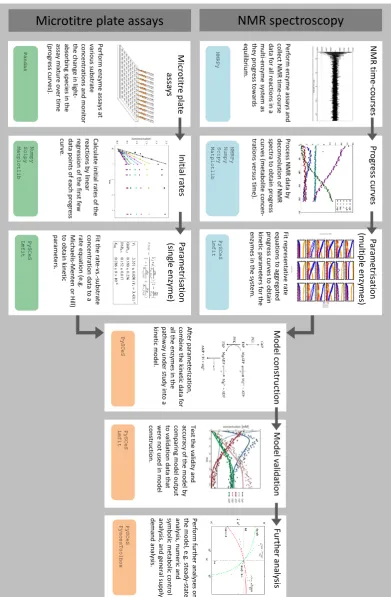
3.1. Workflow for enzyme kinetics for systems biology 167
The main workflow for bottom-up kinetic model construction in systems biology, as described 168
in this paper, is summarised in Figure1. Enzyme kinetic data were obtained in one of two ways:
169
Per fo rm e n zyme as says an d co lle ct N MR ti me -c o u rs e d ata fo r all re ac ti o n s in a mu lti -e n zyme s ys te m as th ey p ro gre ss to w ard s eq u ilib ri u m. N M R time -c ou rses NMRPy
NMR spectroscopy
Microtitre plate assays
Pro ce ss N MR dat a b y d ec o n vo lu ti o n o f N MR sp ec tr a to o b tai n p ro gre ss cu rve s ( me tab o lite c o n ce n -tr ati o n s ve rs u s ti me ). Pr ogr ess cu rv es NMRPy Numpy Scipy Matplotlib Pe rfo rm e n zyme as says at vari o u s s u b str ate co n ce n tr ati o n s an d mo n ito r th e c h an ge in lig h t-ab so rb in g s p ec ie s i n th e as say mix tu re o ve r ti me (p ro gre ss c u rve s). M ic rot it re p la te assa ys Pandas Fit re p re se n tati ve rat e eq u ati o n s to ag gre gate d p ro gre ss c u rve s to o b tai n ki n eti c p arame te rs fo r th e en zyme s i n th e s ys te m. Par ame trisa tion (mu lt ip le en zymes) PySCeS Lmfit A fte r p arame te ri zati o n , co mb in e th e ki n eti c d ata fo r all th e e n zyme s i n th e p ath w ay u n d er stu d y in to a ki n eti c mo d el. M od el con st ru ct ion PySCeS Fu rt h er an aly sis Per fo rm fu rt h er an alys es o n th e mo d el, e .g . st ead y-state an al ys is, n u me ric an d symb o lic me tab o lic c o n tr o l an alys is , an d g en eral s u p p ly -d eman d an alys is . PySCeS PyscesToolbox Te st th e vali d ity an d ac cu racy o f th e mo d el b y co mp ari n g mo d el o u tp u t to vali d ati o n d ata th at w er e n o t u se d in mo d el co n str u cti o n . M od el valid at ion PySCeS Lmfit Fit th e rate -vs .-s u b str ate co n ce n tr ati o n d ata to a rat e e q u ati o n (e .g . Mi ch ae lis -Me n te n o r H ill) to o b tai n ki n eti c p arame te rs . P ar ame trisa tion (single en zy me) PySCeS Lmfit Calcu late in iti al rat es o f th e re ac ti o n s b y lin ear re gre ss io n o f th e fir st few d ata p o in ts o f each p ro gre ss cu rve . In it ial ra tes Numpy Scipy Matplotlib
which were then parametrised by fitting to a system of ODEs with the appropriate enzyme kinetic 171
rate equations; or alternatively, initial-rate kinetics were performed on a single enzyme, typically with 172
a spectrophotometric assay using microtitre plates, and fitted to a rate equation. In this paper, one 173
example of each approach is discussed in detail (Sections3.2–3.4); in general, it needs to be repeated
174
until all of the enzymes in the pathway under study have been characterised. 175
In the next step, all the kinetic rate equations and parameters were assembled into a model of 176
the complete pathway, which was then validated by comparing its output to experimental data that 177
were not used for model construction (Section3.5). The workflow subsequently allowed a number of
178
additional computational analyses to be easily performed on a properly constructed and validated 179
model (Figure1).
180
Each of the above steps is described in greater detail in the following sections, emphasising the 181
role of the Python language in ‘gluing’ the various analyses together. The Python modules that were 182
used for each step are listed at the bottom of each block in Figure1.
183
3.2. Enzyme kinetics from NMR spectroscopy 184
To obtain enzyme-kinetic parameters with NMR spectroscopy, a cell lysate was incubated with 185
substrates, products, cofactors and any allosteric modifiers. A series of NMR spectra was collected over 186
time; the spectra were processed and peaks quantified by deconvolution to yield a series of progress 187
curves, which were then fitted to a kinetic equation or set of equations for the reactions followed. The 188
method [11] can also be applied to purified enzymes.
189
The use of lysates (in contrast to purified enzyme preparations, which only contain the enzyme of 190
interest) required that reaction boundaries be delimited by omitting essential cofactors as appropriate. 191
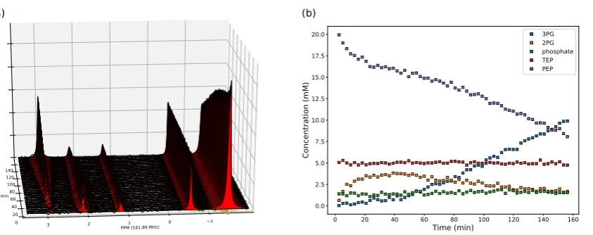
For example, the dataset in Figure2was acquired by incubating aSaccharomyces cerevisiaelysate with
192
phosphoenolpyruvate, leading to the enolase (ENO) and phosphoglycerate mutase (PGM) reactions 193
proceeding in the reverse direction. Subsequent reactions on either side did not proceed because the 194
necessary cofactors (ADP for pyruvate kinase, ATP for phosphoglycerate kinase) were missing. It was 195
important to limit the size of the system of reactions in this way, as fitting too many reactions (and 196
their associated kinetic parameters) at once may lead to unidentifiable parameters [26].
197
Our custom open-source NMR processing Python module, NMRPy [23], facilitates the
198
bulk-processing and quantification of arrayed NMR spectra that are typically produced by such 199
experiments. Figure2provides the raw NMR spectra and quantification of a representative experiment
200
on the PGM-ENO reaction couple, where the reaction was initiated by incubating the lysate with 201
phosphoenolpyruvate. Because this was a31P-NMR experiment, natural substrates could be used,
202
but when performing13C-NMR spectroscopy,13C-labelled substrates have to be used because of the
203
low natural abundance of this NMR-active isotope. The Supplementary Material contains an example 204
Jupyternotebook with code and annotations to read and process the NMR data for Figure2. 205
To fit the kinetic parameters for both enzymes, a number of such experiments had to be performed 206
with different starting concentrations of substrates and/or products. The fitting procedure is described
207
in detail in Section3.4below.
208
3.3. Enzyme kinetics from spectrophotometric assays 209
Enzyme-kinetic parameters were determined from spectrophotometric assays, which were 210
performed on microtitre plates to increase throughput. Initial rates were obtained for different substrate
211
concentrations by linear regression on the initial parts of the reaction progress curves. Where possible, 212
such assays were coupled to reactions producing or consuming NAD(P)H, which has a convenient 213
light absorbance peak at a wavelength of 340 nm and can thus be detected directly with visible-light 214
spectrophotometry. Non-linear regression of the rate-versus-concentration data, using appropriate rate 215
equations, yielded the kinetic constants for the enzyme. 216
Microtitre plate readers typically produce tabulated timeversusabsorbance data, which can be
217
PPM (161.89 MHz)1 0 1 2
3 min.
0 20 40 60 80 100 120 140
(a)
0 20 40 60 80 100 120 140 160
Time (min)
0.0 2.5 5.0 7.5 10.0 12.5 15.0 17.5 20.0
Concentration (mM)
3PG 2PG phosphate TEP PEP
(b)
Figure 2. (a) Array of 31P-NMR spectra from an incubation of S. cerevisiae lysate with phosphoenolpyruvate. Spectra were acquired 2.6 min apart (repetition time) and processed with NMRPy(apodisation, Fourier transform, phase correction and integration by deconvolution). The peak identities are, from left to right: 3-phosphoglycerate (3PG), 2-phosphoglycerate (2PG), phosphate, triethyl phosphate (TEP, internal standard), and phosphoenolpyruvate (PEP). Original spectra are shown as black lines and the deconvoluted peak areas are shown with filled red colour. (b) Quantification of
the spectra after processing withNMRPy. The output from the analysis was concentration-versus-time
data.NMRPycan read raw data from the major NMR instrument vendors and has built-in functions to
display both the arrayed spectra and quantified data. Data and annotated code (Jupyternotebook) are
provided in the Supplementary Material.
these; the data analysis librarypandas[15] (https://pandas.pydata.org) is specifically suited to this task.
219
Jupyternotebooks in conjunction withmatplotlibfor visualisation and plotting provided a powerful 220
single interface for data analyses, including loading and preprocessing data, performing the actual 221
data analysis, visualisation and saving the results. 222
The Supplementary Material contains an annotated exampleJupyternotebook to illustrate the
223
processing of kinetic data acquired with a microtitre plate reader. The following steps were involved: 224
Importing data New dataframes were created inpandasfrom a variety of input formats, including
225
Excel and CSV. Several preprocessing and customisation methods were used (e.g. for the 226
conversion of date/time fields into a format that can be used by Python), as near-perfect tabulated
227
data are rarely produced by the associated software and the formats differ between instrument
228
vendors. 229
Linear regression The absorbance-versus-time data were subject to linear regression over a suitable
230
time range to calculate initial rates. The attachedJupyternotebook provides two tools (using
231
interactivematplotlibgraphs, and usingipywidgets), which were used to efficiently apply this
232
analysis to a large number of datasets. 233
Preprocessing data Thepandaslibrary provided functions to easily normalise the data, either to
234
a single entry, a single row, or an entire dataframe. Further, Python functions were written 235
to automate repetitive processing tasks in a consistent way. Examples of such normalisations 236
included subtraction of blank readings, the conversion of absorbance values to concentrations, or 237
the subtraction of the initial time reading from subsequent time data. 238
Fitting data For fitting of initial rate data to an enzyme-kinetic rate equation (e.g. the Michaelis-Menten
239
equation), the Python packagelmfit[27] provided a high-level interface to various non-linear
240
optimization and curve fitting routines with access to both global and local optimisation 241
algorithms. This is further discussed in Section3.4below.
242
Data Visualization A leading visualisation and 2D-plotting library for Python ismatplotlib, which
243
was used in this analysis because of its powerful and flexible design, its interoperability with 244
0
1
2
3
4
5
6
[NAD
+] (mM)
0.0
0.2
0.4
0.6
0.8
1.0
v (
m
ol/
m
in/
m
g
pr
ot
ein
)
Figure 3.Kinetic characterisation of glucose-6-phosphate dehydrogenase in lysates ofZymomonas mobilis
by initial rate kinetics. Lysates were incubated with a fixed concentration of glucose-6-phosphate and
varying concentrations of NAD+. The graph shows initial rate data for varying NAD+concentrations
(points, mean±SE of triplicate determinations) and the kinetic equation fit (line). Further details and
code are available in the supplementaryJupyternotebook.
3.4. Fitting experimental data to obtain kinetic parameters 246
In the case of initial rate assays on a single enzyme the rate-versus-concentration data for the 247
varying substrate were fitted to an appropriate rate equation by non-linear regression with thelmfit
248
Python module. Figure3shows a fit for the enzyme glucose-6-phosphate dehydrogenase as a function
249
of varying NAD+concentrations. Further details and fitting code are provided in theJupyternotebook
250
in the Supplementary Material. 251
Kinetic parameters were obtained from NMR progress curves in a similar way with a few 252
modifications. An ODE model was created for the system of reactions studied in the NMR assay, 253
using generic rate equations. The kinetic parameters were obtained by fitting the experimental data 254
(concentration time courses) to model simulations for the same time period. While the system of ODEs 255
could in principle be coded directly by hand [18], our simulation softwarePySCeS[19] simplified this
256
task by allowing reaction stoichiometry and rate equations to be intuitively specified in an input file, 257
and by being able to specify directly and easily the time points for which model simulations needed to 258
be output. The fitting was again accomplished with thelmfitmodule.
259
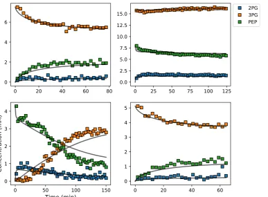
Figure4shows a representative example of four progress curves for the PGM-ENO couple at
260
different starting concentrations of substrates and products, where the arrayed NMR spectra have
261
already been processed to calculate concentration time-courses (see Section3.2). Note that some of the
262
reactions ran in reverse and in one case more than one metabolite was present at the start of the assay. 263
The lines represent the model output with the parameters fitted toallof the datasets, not only those
264
shown here. 265
The Supplementary Material contains aJupyternotebook with the annotated fitting code that
266
provided the fitted parameters and associated error estimates. The workflow allowed for easy-to-follow 267
data processing, from the original NMR FID data to the final fitted parameter values. 268
3.5. Assembly and validation of a larger kinetic model of a pathway 269
Once all the enzymes of a pathway under study have been characterised as described in 270
Sections3.2–3.4, the next step was to combine this information into a kinetic model. The process of
271
bottom-up model construction has been reviewed [10] and will not be repeated in detail here, other
272
0
20
40
60
80
0
2
4
6
0
25
50
75
100
125
0.0
2.5
5.0
7.5
10.0
12.5
15.0
2PG
3PG
PEP
0
50
100
150
Time (min)
0
1
2
3
4
Concentration (mM)
0
20
40
60
0
1
2
3
4
5
Figure 4.Example of experimental and simulated data for the PGM-ENO couple studied by NMR inS. cerevisiaelysates incubated with different starting concentrations of substrates and products. Square symbols represent experimental data and solid lines represent the simulated model data after parameter optimization to all data sets simultaneously. Abbreviations: 2PG, 2-phosphoglycerate; 3PG, 3-phosphoglycerate; PEP, phosphoenolpyruvate.
activities and kinetics, which should all have been determined under the samein vivo-like conditions
274
(e.g. [28,29]). 275
The role of the next step, model validation, was to test the accuracy of the predictions of the model. 276
By investigating how well the model reproducedindependentexperimental data that werenot usedin
277
the model construction process itself (i.e. for fitting the model parameters), this allowed us to assess 278
the quality of the model. 279
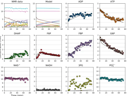
By way of example, Figure5shows the output from a kinetic model ofEscherichia coliglycolysis
280
plotted together with independent metabolite time courses determined in situ using E. coli cells
281
permeabilised with detergent. This time-course experiment was acquired and processed using similar 282
techniques as outlined Section3.2, and is from a whole-pathway study starting with the addition of
283
glucose-6-phosphate and co-factors [23]. The Supplementary Material contains aJupyternotebook
284
with code, model description and data to recreate Figure5.
285
While there were some discrepancies between the data and the model fit, the general agreement 286
was remarkable considering that these are independent validation data. At this point, further analyses 287
could be done, e.g. theχ2 (discrepancy between model and data) could be calculated, or another
288
validation dataset could be plotted and compared to the current one. If different models are available,
289
they can be compared in terms of how well they fit the data [23].
290
These data could also be used to further fit and refine the model. In this case they are no longer 291
independent validation data, and the model would have to be validated against additional independent 292
0 20 40 60 80 0
5 10
15
NMR data
0 20 40 60 80
0 5 10
15
Model
0 20 40 60 80
0 1 2 3 4 5
6
ADP
0 20 40 60 80
0 1 2 3 4
5
ATP
0 20 40 60 80
0 1 2 3 4 5
Concentration (mM)
DHAP
0 20 40 60 80
0 1 2 3 4
5
F6P
0 20 40 60 80
0 1 2 3 4 5
6
FBP
0 20 40 60 80
1 2 3 4 5 6
7
G6P
0 20 40 60 80
Time (min)
7 8 9 10 11 12
13
NAD
+0 20 40 60 80
0 1 2 3 4
5
NADH
0 20 40 60 80
0 1 2 3 4
5
3PG
0 20 40 60 80
9 10 11 12 13 14
15
PO
34Figure 5.Validation of a kinetic model by comparison to independent experimental data. The data
points are quantified NMR time-courses from anin situexperiment with permeabilisedEscherichia
colicells, starting out with 7 mM G6P, 4 mM ATP, 2 mM ADP, 12 mM phosphate, and 10 mM
NAD+. The lines are simulation output from a kinetic model ofE. coliglycolysis, assembled from
kinetic measurements on the individual enzymes as outlined in Sections3.2–3.4. Adapted from [23].
Non-standard abbreviations: DHAP, dihydroxy-acetone phosphate; F6P, fructose-6-phosphate; FBP, fructose-1,6-bisphosphate; G6P, glucose-6-phosphate; 3PG, 3-phosphoglycerate.
3.6. Further model analysis: MCA, GSDA and PyscesToolbox 294
Once a kinetic model for a pathway has been constructed and properly validated, it can be subject 295
to a variety of analyses to gain further insight into its regulatory function. A fundamental example is 296
metabolic control analysis (MCA) [30,31], which aims to quantify the contribution of each of the steps
297
in a pathway to the control of flux or metabolite concentrations, and thus to identify key control points. 298
PySCeShas built-in functions to perform MCA directly. Other analyses, based on MCA, include 299
supply-demand analysis (SDA) [32,33] and its generalised variant GSDA [34], symbolic MCA (SymCA)
300
[35,36], as well as a framework,ThermoKin, that dissects the contributions of thermodynamic and
301
kinetic aspects to enzyme regulation [37].
302
The above-mentioned analysis frameworks have been incorporated into a Python module, 303
PySCeSToolbox[38], which uses theJupyternotebook andIPythonkernel to analyse the models 304
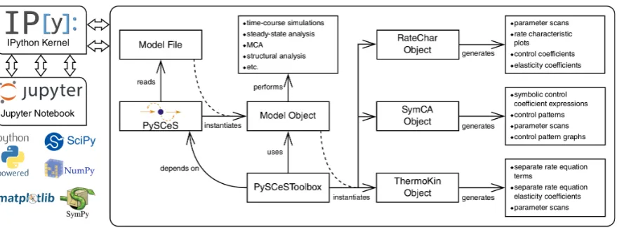
withPySCeSand visualise the output in various interactive ways. Figure6summarises the overall 305
architecture and workflow ofPySCeSToolbox. At the centre of the analysis is aPySCeSmodel object
306
which can be used to instantiate one of three analysis objects: 307
RateChar This module performs GSDA by fixing each variable metabolite in turn (thus making it a 308
system parameter) and varying it below and above its steady-state value. This allows one to 309
Figure 6.PySCeSToolboxarchitecture and workflow.PySCeSinstantiates a model object from file,
which is then used byPySCeSToolboxto instantiate an analysis tool object. The recommended usage
involves running these processes within anIPythonkernel with which the user interacts via theJupyter
notebook. The bottom-left corner shows some of the main technologies used byPySCeSToolbox. Refer
to [38] for details. Reproduced with permission from Christensenet al., Bioinformatics; published by
Oxford University Press, 2018.
was computationally applied [39] to the analysis of published models of pyruvate metabolism in
311
Lactococcus lactis[40] and aspartate-derived amino acid synthesis inArabidopsis thaliana[41]. 312
SymCA This module performs symbolic metabolic control analysis by generating algebraic expressions 313
for the control coefficients in terms of the elasticity coefficients, using theSymPyPython module
314
for symbolic algebra [42]. These expressions are then used to evaluate and visualise so-called
315
control patterns in the network and quantify their relative contribution to the overall value of the 316
control coefficient. A control coefficient can thus be dissected into its most important components.
317
ThermoKin This module calculates, for each reversible reaction in the model, the contribution of 318
thermodynamics and kinetics to the enzyme regulation at a particular steady state using the 319
formalism described in [37]. This contribution may vary as conditions change (e.g. as a result
320
of changes in some model parameters), as the reaction operates closer to or further away from 321
equilibrium. 322
SymCAandThermoKinwere applied [43] to the above-mentioned model of pyruvate metabolism 323
[40]. 324
The main point of this section is to illustrate that fine-grained model analysis can be performed 325
within the same computational framework as the model construction and validation, using Python and 326
Jupyternotebooks; there is no need to change to a new system. The paper describingPySCeSToolbox 327
[38] has example notebooks as supplementary information, illustrating each of the three module
328
functionalities; these will not be repeated here. The detailed model analyses in [39,43] are also
329
accompanied byJupyternotebooks, allowing readers to reproduce the findings.
330
4. Discussion
331
In this paper we have provided examples of applying the powerful capabilities of the Python 332
programming language to systems biology in terms of both computation and data visualisation, 333
making extensive use of theIPythonenvironment andJupyternotebooks as an interactive platform.
334
One compelling aspect of this is the ability to pass information from one Python software to another to 335
create a versatile computational pipeline. For example, experimental data (e.g. in CSV format) can 336
be directly loaded into the shell, restructured into anumpyarray orpandasdata frame, analysed by
337
any number ofscipytools, passed into a computational systems biology software such asPySCeS,
338
and finally visualised using thematplotlibplotting library. While all of these functions are available in
339
within a single environment using scripts that can be automated is incredibly powerful and gives 341
researchers with programming skills a significant advantage. 342
Python is relatively easy to learn compared to other programming languages. The language 343
was designed with a very human-readable format and does not contain the syntactical minutiae of 344
lower level programming languages. This, combined with the excellent freely available resources 345
for learning, makes Python accessible to life-sciences researchers who often have limited computer 346
science training, lowering the barrier of entry and broadening the availability of the analysis platform. 347
In addition to being able to run on different operating systems, Python can integrate with other
348
programming languages and execute Fortran or C code at near-native speeds using the modules 349
f2py[44], which is part ofnumpy, andcython[45] (https://cython.org). This means that increased
350
readability and interpreted code do not have to come at the expense of computational power and 351
speed, as Fortran and C code can be readily wrapped to run natively in Python by using “interfaces to 352
low-level high-performance software in a high-level programming environment” [44]. For example,
353
for ourPySCeSsoftware [19] we have wrapped two additional Fortran solvers that are not part of
354
the standardscipydistribution. Furthermore, the interpreted nature of Python allows scripts to easily
355
be transferred between collaborators without recompiling, meaning that script can be executed on 356
machines with different architectures to produce identical results. This greatly facilitates collaborations
357
between groups and simplifies collaborations within groups. 358
There are many purpose built proprietary software packages for performing the types of analysis 359
described in this paper. These range from general-purpose mathematical analysis and simulation 360
packages such as Mathematica (http://www.wolfram.com/mathematica) or MATLAB (https://www.
361
mathworks.com/products/matlab.html) to dedicated analysis software provided by instrument vendors. 362
While these programs are usually excellent at performing the tasks for which they were designed, the 363
fact that they are closed-source limits their extensibility. 364
In contrast, the Python programming language and the libraries described in this paper are 365
open-source. The Open Source Initiative (OSI,https://opensource.org/) is an organisation that promotes
366
awareness and adoption of open-source software and protects open-source communities of practice. 367
Open-source software development is a system of collaboration where loosely affiliated contributors
368
work towards a common software goal or innovation, making the source codes of these projects 369
available to the public. Python and the OSI are inextricably linked; the founder of Python, Guido 370
van Rossum, has served on the OSI board of Directors and championed the movement by organising 371
‘sprint’ events, often following Python conventions such as PyCon (http://www.pycon.org/), where
372
programmers work on a variety of open- source projects. This approach extends to the scientific Python 373
community, which organises annual SciPy and EuroSciPy conferences (https://conference.scipy.org/).
374
Python has a healthy, active and supportive community, which facilitates its adoption. This creates a 375
feed-forward mechanism where researchers can work and develop new tools in Python because these 376
can be easily integrated into existing software pipelines. 377
The workflow described in this paper latches on to the above feed-forward mechanism by 378
integrating various tools. As such, the list is by no means exhaustive but rather a collection of examples 379
that we use in day-to-day analyses. We do not claim that Python is the best, nor is the aim of this paper 380
to provide a systematic comparison of programming languages or tools; rather, it is an illustration 381
of an adaptable and expandable workflow that has proven useful in our hands. In addition, while 382
our examples in the Supplementary Material are presented asJupyternotebooks, this is not a strict
383
requirement and the analysis could have been performed with a series of Python scripts. The interactive 384
nature ofJupyter, as well as its capabilities for annotation, structuring and visualisation, just provided
385
additional functionality. 386
To further substantiate the case for Python in systems biology, we note that, while we have 387
focussed in this paper on those programs and libraries that are most frequently used in our group, 388
researchers have a wide choice of software, many of which are either written in Python or expose a 389
Python API (summarised in the SBML software matrix, seehttp://sbml.org/SBML_Software_Guide/
SBML_Software_Matrix). Each of these programs is dedicated to particular analysis tasks, and they 391
will not all be covered in detail here. To mention only a few in addition to the libraries listed in 392
Section2.2.1,modelbase[46] has a focus on kinetic modelling similar toPySCeS, whileCOBRAPy
393
[47] andCBMPy(http://cbmpy.sourceforge.net/) have a focus on constraint-based modelling of large
394
stoichiometric networks.ScrumPy[48] can do both, but has a focus on constraint-based modelling.
395
Importantly, by working in a Python environment, the user has the flexibility to interact with any of 396
these programs as required and to easily create new workflows. 397
In the field of systems biology, new software and technical developments have led to an exponential 398
growth in the rate of experimental data generation, particularly via high throughput methods [49], as
399
well as the number and complexity of computational tools. Concomitantly, the importance of sharing 400
data and resources is increasingly being recognised. Computational systems biology models are 401
curated and stored in databases such as JWS Online [50] and BioModels [9]. Moreover, standards such
402
as SBML [20] facilitate exchange of models across simulation tools. The need to share, exchange and
403
reuse data led to the development of the FAIRDOM project [51], which aims to develop frameworks
404
and guidelines to make data more Findable, Accessible, Interoperable and Reusable. This project 405
has produced the FAIRDOMHub which uses the SEEK [52] open-source web platform with tools for
406
collating and annotating datasets, models, simulations and research outcomes. SEEK has a JavaScript 407
Object Notation (JSON) API for uploading and downloading files, and Python supports JSON natively, 408
facilitating integration into Python workflows. 409
5. Conclusions
410
We have demonstrated how the Python programming language can act as a glue to interface 411
between different analysis tools required for the construction, validation and analysis of kinetic models
412
in bottom-up systems biology. Our workflow enables investigators to focus on the scientific problem 413
instead of issues of data integration between platforms. TheJupyternotebook is an ideal e-labbook
414
and allows the user to keep everything related to a particular analysis in one place, including raw data, 415
graphical output and descriptive annotations. 416
Supplementary Materials:The following are available at
417
http://www.mdpi.com//xx/1/5/s1, Document S1: Instructions for Running Supplementary Notebooks;
418
http://www.mdpi.com//xx/1/5/s2, Archive S2: ZIP archive with supplementary notebooks and associated data files.
419
Author Contributions: conceptualization, J.M.R.; methodology, C.J.S, C.T.v.S., J.W., J.M.R.; software, C.J.S.,
420
C.T.V.S., J.W., J.M.R.; validation, M.B., C.J.B.; formal analysis, C.J.S, C.T.v.S., J.W.; investigation, C.J.S, C.T.v.S., J.W.;
421
resources, J.M.R.; data curation, M.B., C.J.B.; writing–original draft preparation, all authors; writing–review and
422
editing, J.M.R., C.J.B.; visualization, M.B., C.J.S., J.W., J.M.R.; supervision, J.M.R.; project administration, J.M.R.;
423
funding acquisition, J.M.R.
424
Funding:This research was funded by the National Research Foundation (South Africa), grant numbers 93466,
425
93670, and 114748, as well as by Stellenbosch University (student scholarships to CJS and MB). The APC was
426
funded in part from the Open Access Publication Fund of Stellenbosch University.
427
Conflicts of Interest: The authors declare no conflict of interest. The funders had no role in the design of the
428
study; in the collection, analyses, or interpretation of data; in the writing of the manuscript, or in the decision to
429
publish the results.
430
Abbreviations
431
The following abbreviations are used in this manuscript:
API Application Programming Interface
ENO Enolase
FID Free Induction Decay
GSDA Generalised Supply-Demand Analysis
JSON JavaScript Object Notation
MCA Metabolic Control Analysis
NMR Nuclear Magnetic Resonance
ODE Ordinary Differential Equation
OSI Open Source Initiative
PGM Phosphoglycerate Mutase
SBML Systems Biology Markup Language
SDA Supply-Demand Analysis
434
References
435
1. Kitano, H. International alliances for quantitative modeling in systems biology. Mol. Syst. Biol. 2005,
436
1, 2005.0007. doi:10.1038/msb4100011.
437
2. Westerhoff, H.V.; Alberghina, L. Systems Biology: Did we know it all along?; Springer-Verlag: Berlin, 2005;
438
pp. 3–9. doi:10.1007/b137744.
439
3. Snoep, J.L.; Bruggeman, F.; Olivier, B.G.; Westerhoff, H.V. Towards building the silicon cell: a modular
440
approach. Biosystems2006,83, 207–216. doi:10.1016/j.biosystems.2005.07.006.
441
4. Bruggeman, F.J.; Westerhoff, H.V. The nature of systems biology. Trends Microbiol. 2007, 15, 45–50.
442
doi:10.1016/j.tim.2006.11.003.
443
5. Rohwer, J.M.; Hanekom, A.J.; Crous, C.; Snoep, J.L.; Hofmeyr, J.H.S. Evaluation of a simplified generic
444
bi-substrate rate equation for computational systems biology. IEE Proc. Syst. Biol.2006,153, 338–341.
445
6. Rohwer, J.M.; Hanekom, A.J.; Hofmeyr, J.H.S. A universal rate equation for systems biology. Experimental
446
Standard Conditions of Enzyme Characterizations. Proceedings of the 2nd International Beilstein Workshop;
447
Hicks, M.G.; Kettner, C., Eds.; Beilstein-Institut zur Förderung der Chemischen Wissenschaften: Frankfurt,
448
2007; pp. 175–187.
449
7. Kholodenko, B.N.; Demin, O.V.; Moehren, G.; Hoek, J.B. Quantification of short term signaling by the
450
epidermal growth factor receptor. J. Biol. Chem.1999,274, 30169–30181. doi:10.1074/jbc.274.42.30169.
451
8. van Niekerk, D.D.; Penkler, G.P.; du Toit, F.; Snoep, J.L. Targeting glycolysis in the malaria parasite
452
Plasmodium falciparum. FEBS J.2016,283, 634–646. doi:10.1111/febs.13615.
453
9. le Novère, N.; Bornstein, B.; Broicher, A.; Courtot, M.; Donizelli, M.; Dharuri, H.; Li, L.; Sauro, H.; Schilstra,
454
M.; Shapiro, B.; Snoep, J.L.; Hucka, M. BioModels Database: a free, centralized database of curated,
455
published, quantitative kinetic models of biochemical and cellular systems. Nucleic Acids Res. 2006,
456
34, D689–D691. doi:10.1093/nar/gkj092.
457
10. Rohwer, J.M. Kinetic modelling of plant metabolic pathways. J. Exp. Bot. 2012, 63, 2275–2292.
458
doi:10.1093/jxb/ers080.
459
11. Eicher, J.J.; Snoep, J.L.; Rohwer, J.M. Determining enzyme kinetics for systems biology with Nuclear
460
Magnetic Resonance spectroscopy. Metabolites2012,2, 818–843. doi:10.3390/metabo2040818.
461
12. Oliphant, T.E. Python for scientific computing.Comput. Sci. Eng.2007,9, 10–20. doi:10.1109/MCSE.2007.58.
462
13. van der Walt, S.; Colbert, S.C.; Varoquaux, G. The NumPy array: a structure for efficient numerical
463
computation. Comput. Sci. Eng.2011,13, 22–30. doi:10.1109/MCSE.2011.37.
464
14. Jones, E.; Oliphant, T.; Peterson, P.; others. SciPy: Open source scientific tools for Python, 2001–.
465
15. McKinney, W. Data Structures for Statistical Computing in Python. Proceedings of the 9th Python in
466
Science Conference; van der Walt, S.; Millman, J., Eds., 2010, pp. 51–56.
467
16. Hunter, J.D. Matplotlib: A 2D graphics environment. Computing In Science & Engineering2007,9, 90–95.
468
doi:10.1109/MCSE.2007.55.
469
17. Anaconda Software Distribution. Computer Software, 2017. Vers. 2-2.4.0, https://www.anaconda.com.
470
18. Olivier, B.G.; Rohwer, J.M.; Hofmeyr, J.H.S. Modelling cellular processes with Python and SciPy. Mol. Biol.
471
Rep.2002,29, 249–254.
472
19. Olivier, B.G.; Rohwer, J.M.; Hofmeyr, J.H.S. Modelling cellular systems with PySCeS.Bioinformatics2005,
473
21, 560–561.
20. Hucka, M.; Finney, A.; Sauro, H.M.; Bolouri, H.; Doyle, J.C.; Kitano, H.; Arkin, A.P.; Bornstein, B.J.; Bray, D.;
475
Cornish-Bowden, A.; Cuellar, A.A.; Dronov, S.; Gilles, E.D.; Ginkel, M.; Gor, V.; Goryanin, I.I.; Hedley, W.J.;
476
Hodgman, T.C.; Hofmeyr, J.H.; Hunter, P.J.; Juty, N.S.; Kasberger, J.L.; Kremling, A.; Kummer, U.; Novère,
477
N.L.; Loew, L.M.; Lucio, D.; Mendes, P.; Minch, E.; Mjolsness, E.D.; Nakayama, Y.; Nelson, M.R.; Nielsen,
478
P.F.; Sakurada, T.; Schaff, J.C.; Shapiro, B.E.; Shimizu, T.S.; Spence, H.D.; Stelling, J.; Takahashi, K.; Tomita,
479
M.; Wagner, J.; Wang, J. The systems biology markup language (SBML): a medium for representation and
480
exchange of biochemical network models. Bioinformatics2003,19, 524–531.
481
21. Hoops, S.; Sahle, S.; Gauges, R.; Lee, C.; Pahle, J.; Simus, N.; Singhal, M.; Xu, L.; Mendes,
482
P.; Kummer, U. COPASI–a COmplex PAthway SImulator. Bioinformatics 2006, 22, 3067–3074.
483
doi:10.1093/bioinformatics/btl485.
484
22. Somogyi, E.T.; Bouteiller, J.M.; Glazier, J.A.; König, M.; Medley, J.K.; Swat, M.H.; Sauro, H.M.
485
libRoadRunner: a high performance SBML simulation and analysis library. Bioinformatics 2015,
486
31, 3315–3321. doi:10.1093/bioinformatics/btv363.
487
23. Eicher, J.J. Understanding Glycolysis inEscherichia coli: a Systems Approach using Nuclear Magnetic
488
Resonance Spectroscopy. PhD thesis, Stellenbosch University, 2013.
489
24. Pérez, F.; Granger, B.E. IPython: a system for interactive scientific computing. Comput. Sci. Eng.2007,
490
9, 21–29. doi:10.1109/MCSE.2007.53.
491
25. Kluyver, T.; Ragan-Kelley, B.; Pérez, F.; Granger, B.E.; Bussonnier, M.; Frederic, J.; Kelley, K.; Hamrick,
492
J.B.; Grout, J.; Corlay, S.; Ivanov, P.; Avila, D.; Abdalla, S.; Willing, C.; others. Jupyter Notebooks – a
493
publishing format for reproducible computational workflows; IOS Press: Amsterdam, 2016; pp. 87–90.
494
doi:10.3233/978-1-61499-649-1-87.
495
26. Ashyraliyev, M.; Fomekong-Nanfack, Y.; Kaandorp, J.A.; Blom, J.G. Systems biology: parameter estimation
496
for biochemical models. FEBS J.2009,276, 886–902.
497
27. Newville, M.; Stensitzki, T.; Allen, D.B.; Ingargiola, A. LMFIT: Non-linear least-square minimization and
498
curve-fitting for Python. Zenodo, 2014. doi:10.5281/zenodo.11813.
499
28. van Eunen, K.; Bouwman, J.; Daran-Lapujade, P.; Postmus, J.; Canelas, A.B.; Mensonides, F.I.C.;
500
Orij, R.; Tuzun, I.; van den Brink, J.; Smits, G.J.; van Gulik, W.M.; Brul, S.; Heijnen, J.J.; de Winde,
501
J.H.; de Mattos, M.J.T.; Kettner, C.; Nielsen, J.; Westerhoff, H.V.; Bakker, B.M. Measuring enzyme
502
activities under standardizedin vivo-like conditions for systems biology. FEBS J.2010,277, 749–760.
503
doi:10.1111/j.1742-4658.2009.07524.x.
504
29. García-Contreras, R.; Vos, P.; Westerhoff, H.V.; Boogerd, F.C. Whyin vivomay not equalin vitro– new
505
effectors revealed by measurement of enzymatic activities under the samein vivo-like assay conditions.
506
FEBS J.2012,279, 4145–4159. doi:10.1111/febs.12007.
507
30. Kacser, H.; Burns, J.A. The control of flux. Symp. Soc. Exp. Biol.1973,27, 65–104.
508
31. Heinrich, R.; Rapoport, T.A. A linear steady-state treatment of enzymatic chains. General properties,
509
control and effector strength. Eur. J. Biochem. 1974,42, 89–95.
510
32. Hofmeyr, J.H.S.; Cornish-Bowden, A. Regulating the cellular economy of supply and demand. FEBS Lett.
511
2000,476, 47–51.
512
33. Hofmeyr, J.H.S.; Rohwer, J.M. Supply-demand analysis: a framework for exploring the regulatory design
513
of metabolism. Methods Enzymol.2011,500, 533–554. doi:10.1016/B978-0-12-385118-5.00025-6.
514
34. Rohwer, J.M.; Hofmeyr, J.H.S. Identifying and characterising regulatory metabolites with generalised
515
supply-demand analysis. J. Theor. Biol.2008,252, 546–554. doi:10.1016/j.jtbi.2007.10.032.
516
35. Reder, C. Metabolic control theory: A structural approach. J. Theor. Biol.1988,135, 175–201.
517
36. Hofmeyr, J.H.S. Metabolic control analysis in a nutshell. Proceedings of the 2nd International Conference
518
on Systems Biology; Yi, T.M.; Hucka, M.; Morohashi, M.; Kitano, H., Eds.; Omnipress: Madison, WI, USA,
519
2001; pp. 291–300.
520
37. Rohwer, J.M.; Hofmeyr, J.H.S. Kinetic and thermodynamic aspects of enzyme control and regulation. J.
521
Phys. Chem. B2010,114, 16280–16289. doi:10.1021/jp108412s.
522
38. Christensen, C.D.; Hofmeyr, J.H.S.; Rohwer, J.M. PySCeSToolbox: a collection of metabolic pathway
523
analysis tools. Bioinformatics2018,34, 124–125. doi:10.1093/bioinformatics/btx567.
524
39. Christensen, C.D.; Hofmeyr, J.H.S.; Rohwer, J.M. Tracing regulatory routes in metabolism using generalised
525
supply-demand analysis. BMC Syst. Biol.2015,9, 89. doi:10.1186/s12918-015-0236-1.
40. Hoefnagel, M.H.N.; Starrenburg, M.J.C.; Martens, D.E.; Hugenholtz, J.; Kleerebezem, M.; Swam,
527
I.I.V.; Bongers, R.; Westerhoff, H.V.; Snoep, J.L. Metabolic engineering of lactic acid bacteria, the
528
combined approach: kinetic modelling, metabolic control and experimental analysis. Microbiology2002,
529
148, 1003–1013.
530
41. Curien, G.; Bastien, O.; Robert-Genthon, M.; Cornish-Bowden, A.; Cárdenas, M.L.; Dumas, R.
531
Understanding the regulation of aspartate metabolism using a model based on measured kinetic parameters.
532
Mol. Syst. Biol.2009,5, 271. doi:10.1038/msb.2009.29.
533
42. Meurer, A.; Smith, C.P.; Paprocki, M.; ˇCertík, O.; Kirpichev, S.B.; Rocklin, M.; Kumar, A.; Ivanov, S.;
534
Moore, J.K.; Singh, S.; Rathnayake, T.; Vig, S.; Granger, B.E.; Muller, R.P.; Bonazzi, F.; Gupta, H.; Vats,
535
S.; Johansson, F.; Pedregosa, F.; Curry, M.J.; Terrel, A.R.; Rouˇcka, v.; Saboo, A.; Fernando, I.; Kulal, S.;
536
Cimrman, R.; Scopatz, A. SymPy: symbolic computing in Python. PeerJ Comput. Sci. 2017,3, e103.
537
doi:10.7717/peerj-cs.103.
538
43. Christensen, C.D.; Hofmeyr, J.H.S.; Rohwer, J.M. Delving deeper: Relating the behaviour of a metabolic
539
system to the properties of its components using symbolic metabolic control analysis. PLoS One2018,
540
13, e0207983. doi:10.1371/journal.pone.0207983.
541
44. Peterson, P. F2PY: a tool for connecting Fortran and Python programs. Int. J. Comput. Sci. Eng.2009,4, 296.
542
doi:10.1504/ijcse.2009.029165.
543
45. Dalcin, L.; Bradshaw, R.; Smith, K.; Citro, C.; Behnel, S.; Seljebotn, D. Cython: the best of both worlds.
544
Comput. Sci. Eng.2011,13, 31–39. doi:10.1109/MCSE.2010.118.
545
46. Ebenhöh, O.; van Aalst, M.; Saadat, N.P.; Nies, T.; Matuszy ´nska, A. Building mathematical models of
546
biological systems with modelbase. Journal of Open Research Software2018,6. doi:10.5334/jors.236.
547
47. Ebrahim, A.; Lerman, J.A.; Palsson, B.O.; Hyduke, D.R. COBRApy: COnstraints-Based Reconstruction and
548
Analysis for Python. BMC Syst. Biol.2013,7, 74. doi:10.1186/1752-0509-7-74.
549
48. Poolman, M.G. ScrumPy: metabolic modelling with Python. Syst. Biol. (Stevenage)2006,153, 375–378.
550
49. Cook, C.E.; Bergman, M.T.; Finn, R.D.; Cochrane, G.; Birney, E.; Apweiler, R. The European
551
Bioinformatics Institute in 2016: Data growth and integration. Nucleic Acids Res. 2016,44, D20–D26.
552
doi:10.1093/nar/gkv1352.
553
50. Olivier, B.G.; Snoep, J.L. Web-based kinetic modelling using JWS Online. Bioinformatics2004,20, 2143–2144.
554
doi:10.1093/bioinformatics/bth200.
555
51. Wolstencroft, K.; Krebs, O.; Snoep, J.L.; Stanford, N.J.; Bacall, F.; Golebiewski, M.; Kuzyakiv, R.; Nguyen, Q.;
556
Owen, S.; Soiland-Reyes, S.; Straszewski, J.; van Niekerk, D.D.; Williams, A.R.; Malmström, L.; Rinn, B.;
557
Müller, W.; Goble, C. FAIRDOMHub: a repository and collaboration environment for sharing systems
558
biology research. Nucleic acids research2017,45, D404–D407. doi:10.1093/nar/gkw1032.
559
52. Wolstencroft, K.; Owen, S.; Krebs, O.; Nguyen, Q.; Stanford, N.J.; Golebiewski, M.; Weidemann, A.;
560
Bittkowski, M.; An, L.; Shockley, D.; Snoep, J.L.; Mueller, W.; Goble, C. SEEK: a systems biology data and
561
model management platform. BMC Syst. Biol.2015,9, 33. doi:10.1186/s12918-015-0174-y.