Joint communication and positioning based on soft channel parameter estimation

(1)

R E S E A R C H

Open Access

Joint communication and positioning based on

soft channel parameter estimation

Kathrin Schmeink

*

, Rebecca Adam and Peter Adam Hoeher

Abstract

A joint communication and positioning system based on maximum-likelihood channel parameter estimation is proposed. The parameters of the physical channel, needed for positioning, and the channel coefficients of the equivalent discrete-time channel model, needed for communication, are estimated jointly using a priori

information about pulse shaping and receive filtering. The paper focusses on the positioning part of the system. It is investigated how soft information for the parameter estimates can be obtained. On the basis of confidence regions, two methods for obtaining soft information are proposed. The accuracy of these approximative methods depends on the nonlinearity of the parameter estimation problem, which is analyzed by so-called curvature measures. The performance of the two methods is investigated by means of Monte Carlo simulations. The results are compared with the Cramer-Rao lower bound. It is shown that soft information aids the positioning. Negative effects caused by multipath propagation can be mitigated significantly even without oversampling.

1 Introduction

Interest in joint communication and positioning is stea-dily increasing [1]. Synergetic effects like improved resource allocation and new applications like location-based services or a precise location determination of emergency calls are attractive features of joint commu-nication and positioning. Since the system requirements of communication and positioning are quite different, it is a challenging task to combine them: Communication aims at high data rates with little training overhead. Only the channel coefficients of the equivalent discrete-time channel model, which includes pulse shaping and receive filtering in addition to the physical channel, need to be estimated for data detection. In contrast, positioning aims at precise position estimates. Therefore, parameters of the physical channel like the time of arri-val (TOA) or the angle of arriarri-val (AOA) need to be esti-mated as accurately as possible [2,3]. Significant training is typically spent for this purpose.

In this paper, a joint communication and positioning system based on maximum-likelihood channel para-meter estimation is suggested [4]. The estimator exploits the fact that channel and parameter estimation are clo-sely related. The parameters of the physical channel and

the channel coefficients of the equivalent discrete-time channel model are estimated jointly by utilizing a priori information about pulse shaping and receive filtering. Hence, training symbols that are included in the data burst aid both communicationandpositioning.

On the one hand, in [5-7], it is proposed to use a priori information about pulse shaping and receive fil-tering in order to improve the estimates of the equiva-lent discrete-time channel model. However, the information about the physical channel is neglected in these publications. On the other hand, channel sounding is performed in order to estimate the parameters of the physical channel [8-10]. But, to the authors best knowl-edge, the proposed parameter estimation methods are not applied for estimation of the equivalent discrete-time channel model. The estimator proposed in this paper combines both approaches: Channel estimation is mandatory for communication purposes. By exploiting a priori information about pulse shaping and receive fil-tering, the channel coefficients can be estimated more preciselyand positioning is enabled. Hence, synergy is created.

This paper focusses on the positioning part of the pro-posed joint communication and positioning system. Most positioning methods suffer from a bias introduced by multipath propagation. Multipath mitigation is, thus, an important issue. The proposed channel parameter

* Correspondence: [email protected]

Information and Coding Theory Lab Faculty of Engineering, University of Kiel Kaiserstrasse 2, 24143 Kiel, Germany

(2)

estimator performs multipath mitigation in two ways: First, the maximum-likelihood estimator is able to take all relevant multipath components into account in order to minimize the modeling error. Second, soft informa-tion can be obtained for the parameter estimates. Soft information corresponds to the variance of an estimate and is a measure of reliability. This information can be exploited by a weighted positioning algorithm in order to improve the accuracy of the position estimate.

On the basis of confidence regions, two different methods for obtaining soft information are proposed: The first method is based on a linearization of the non-linear parameter estimation problem and the second method is based on the likelihood concept. For linear estimation problems, an exact covariance matrix can be determined in closed form. For nonlinear estimation problems, as it is the case for channel parameter estima-tion, there are different approximations to the covar-iance matrix, which are based on a linearization. These approximate covariance matrices are generated by most nonlinear least-squares solvers (e.g., Levenberg-Mar-quardt method) anyway and can be used after further analysis [11]. Confidence regions based on the likelihood method are more robust than those based on approxi-mate covariance matrices since they do not rely on a linearization, but they are also more complex to calcu-late. Heuristic optimization methods like genetic algo-rithms or particle swarm optimization offer a comfortable procedure to determine the likelihood con-fidence region as demonstrated in [12]. Both methods are only approximate, and their accuracy depends on the nonlinearity of the estimation problem. In [13], Bates and Watts introduce curvature measures that indi-cate the amount of nonlinearity. These measures can be used to diagnose the accuracy of the proposed methods.

The remainder of this paper is organized as follows: The system and channel model is described in Section 2. The relationship between channel and parameter

estimation is explained and the nonlinear metric of the maximum-likelihood estimator is derived. General aspects concerning nonlinear optimization are discussed. In Section 3, the concept of soft information is intro-duced. Based on confidence regions, two methods for obtaining soft information concerning the parameter estimates are proposed. In order to further analyze the proposed methods, the curvature measures of Bates and Watts are introduced in Section 4. The curvature mea-sures are calculated for the parameter estimation pro-blem and a first analysis of the propro-blem is given. Afterward, positioning based on the TOA is explained in Section 5, and the performance of the two soft infor-mation methods is investigated by means of Monte Carlo simulations. The results are compared with the Cramer-Rao lower bound. Finally, conclusions are drawn in Section 6.

2 System Concept

2.1 System and channel model

Throughout this paper, the discrete-time complex base-band notation is used. Letx[k] denote thekth modulated and coded symbol of a data burst of lengthK. Some sym-bolsx[k] are known at the receiver side ("training sym-bols”), whereas others are not known ("data symbols”). It is assumed that data and training symbols can be sepa-rated perfectly at the receiver side. The received sampley

[k] at time indexkcan be written as

y[k] =

L

l=0

hl[k]·x[k−l] +n[k], 0≤k≤K+L−1, (1)

wherehl[k] is thelth channel coefficient of the

equiva-lent discrete-time channel model with effective channel memory length L, andn[k] is a Gaussian noise sample with zero mean and variance σ2

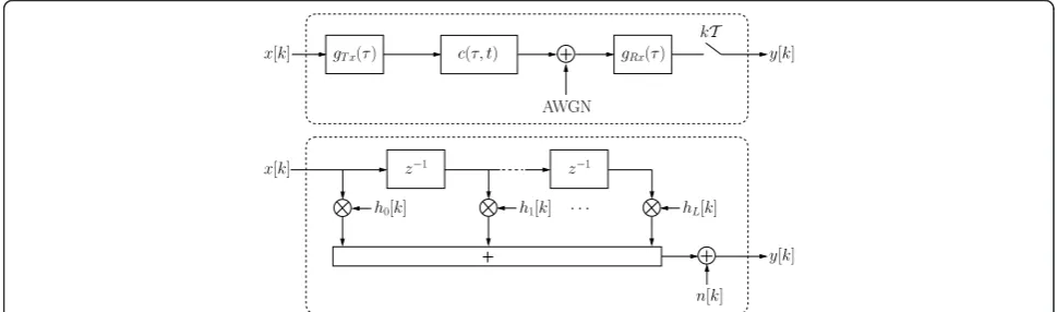
n. The noise process is assumed to be white. In Figure 1, the relationship between the physical channel and the equivalent

c(τ, t)

h0[k]

z−1

hL[k] z−1

h1[k] · · ·

x[k]

n[k] AWGN

kT

y[k]

gRx(τ) gT x(τ)

(3)

discrete-time channel model is shown. The input/output behavior of the continuous-time channel is exactly

represented by the equivalent discrete-time channel model, which is described by an FIR filter with coeffi-cientshl [k]. The delay elements z-1correspond to the

sampling rate _T1. In this paper, only symbol-rate sam-pling T =Ts is considered, whereTsis the symbol

dura-tion.aThe channel coefficientshl [k] are samples of the

overall impulse response of the continuous-time chan-nel. This impulse response is given by the convolution of the known pulse shaping filter g(τ) = gTx(τ), the

unknown physical channelc(τ,t), and the known receive filter gRx(τ). Since the convolution is associative and

commutative, pulse shaping and receive filtering can be combined: g(τ) = gTx(τ) * gRx(τ), where * denotes the

convolution.

The physical channel can be modeled by a weighted sum of delayed Dirac impulses:

c(τ,t) =

M

μ=1

fμ(t)·δ(τ−τμ(t)), (2)

where M is the number of resolvable propagation paths. The parametersfμ(t) andτμ(t) denote the complex amplitude and the propagation delay of theμth path at time t, respectively. Without loss of generality, it is assumed that the multipath components are sorted according to ascending delay:τ1(t) <τ2(t) < ··· <τM(t). The

delay of the first arriving path is called TOA. Positioning is based on the assumption that the TOA corresponds to the distance between transmitter and receiver. This is only true if a line-of-sight (LOS) path exists. In urban or indoor environments, the LOS path is often blocked. In these so-called non-LOS (NLOS) scenarios, the model-ing error reduces the positionmodel-ing accuracy significantly. Additionally, positioning typically suffers from a bias introduced by multipath propagationevenif a LOS path exists. In order to analyze the multipath mitigation abil-ity of the proposed soft channel parameter estimator, this paper restricts itself to LOS scenarios. However, the influence of NLOS is discussed in Section 5.2.

Given c(τ, t) and g(τ), the overall channel impulse responseh(τ,t) can be written as

h(τ,t) =c(τ,t)∗g(τ) =

M

μ=1

fμ(t)·g(τ−τμ(t)). (3)

After symbol-rate sampling (3) att = kTs, the channel

coefficients can be represented as:

hl[k] =

M

μ=1

f_μ[k]·g(lTs−τ_μ[k]). (4)

In the following, it is assumed that the channel is quasi time-invariant over the training length (block fad-ing). Thus, the time indexkin (4) can be omitted.

For simulation of communication systems, it is suffi-cient to consider excess delays. Without loss of general-ity, τ1 = 0 can be assumed then. The effective channel

memory lengthLis, therefore, determined by the excess delayτM–τ1 plus the effective widthTgofg(τ).

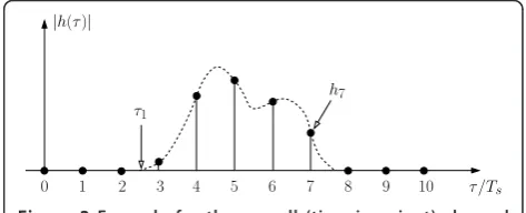
In case of positioning based on the TOA, however, it is important taking into account that τ1= d_c, wheredis the distance between transmitter and receiver and cis the speed of light. Denoting the maximum possible delay by τMmax, the maximum possible channel memory length can be pre-calculated according to

L=

_τmax

M +Tg

Ts

. (5)

This channel memory length covers all possible propa-gation scenarios including the worst case. Hence, the channel impulse response is embedded in a sequence of zeros as shown in Figure 2.

2.2 Channel parameter estimation

Channel estimation is mandatory for data detection. Typically, training symbols are inserted in the data burst for estimation of the equivalent discrete-time channel model. If the channel is quasi time-invariant over the training sequence (block fading), least-squares channel estimation (LSCE) can be applied. In this paper, a training preamble of lengthKtis assumed. For

the interval L ≤ k ≤ Kt - 1, the received samples

according to (1) can be expressed in vector/matrix notation as

y=Xh+n, (6)

whereXis the training matrix with Toeplitz structure,

y= [y[L], y[L+ 1],...,y[Kt- 1]]T is the observation

vec-tor, h=[h0, h1,..., hL]Tis the channel coefficient vector,

and n is a zero mean Gaussian noise vector with

τ/Ts

|h(τ)|

2 3 4 5 6 7 8 9 10

1

τ₁

h₇

0

(4)

covariance matrix Cn=σn2I. The least-squares channel estimates are given by

h=XHX−1XHy=h+ε. (7)

Using the assumptions above, the estimation errorεis zero mean and Gaussian with covariance matrix C_ε=σ_n2XHX−1[14]. For a pseudo-random training sequence, the matrix (XH X) becomes a scaled identity matrix with scaling factor Kt - L, and the covariance

matrix of the estimation error reduces to

Cε = σn2

Kt−LI=σ

2

εI.

The main idea of joining communication and posi-tioning is based on the relationship in (4). If the para-meters of the physical channel are stacked into a vector θ =[Re{f1}, Im{f1},τ1, Re{f2}, ..., τM], (4) can be rewritten

The parameters θ can be estimated by fitting the model function (8) to the least-squares channel esti-mates hl. Hence, the channel estimates are not only used for data detection, but they are also exploited for positioning. Furthermore, refined channel estimates ĥl

are obtained by evaluating (8) for the parameter esti-mate _θˆ[4].b On the one hand, positioning is enabled since the TOAτ1is estimated. On the other hand, data

detection can be improved because refined channel esti-mates are obtained.

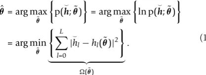
The maximum-likelihood estimate _θˆ is given by the setθthat maximizes the likelihood function [14]

p(h;θ) =

For LSCE with pseudo-random training, this is equiva-lent to maximizing the likelihood function

p(y;θ) =

with respect to θ. The second approach in (10) may seem more natural to some readers since the parameters are estimated directly from the received samples. But since both approaches are equivalent, as proven in the

“Appendix”, it seems more convenient to the authors to apply the first approach: Channel estimates are usually already available in communication systems and the metric derived from (9) is less complex than the metric derived from (10). Hence, only the first approach is con-sidered in the following.

Since the noise is assumed to be Gaussian, the maxi-mum-likelihood estimator corresponds to the least-squares estimator:

The minimization of the metric ₍_θ˜) in (11) cannot be solved in closed form since (θ˜) is nonlinear. An optimization method has to be applied. In order to chose a suitable optimization method to find _θˆ, differ-ent system aspects have to be taken into account, and a tradeoff depending on the requirements has to be found. The goal is to find theglobalminimum of (θ˜). Unfortunately, (θ˜) has manylocal minima due to the superposition of random multipath components. Conse-quently, the optimization method of choice should be either a global optimization method or a local optimiza-tion method in combinaoptimiza-tion with a good initial guess, i. e., an initial guess that is sufficiently close to the global optimum. Both choices involve different benefits and drawbacks. To find a good initial guess is difficult and, therefore, may be seen as a drawback itself. But in case a priori knowledge in form of a good initial guess is available, a search in the complete search space would be unnecessary.

For channel parameter estimation, it is suggested to divide the problem into an acquisition and a tracking phase. In the acquisition phase, a global optimization method is applied, and in the tracking phase, the para-meter estimate of the last data burst may be used as an initial guess for a local optimization method. This is sui-table for channels that do not change too rapidly from data burst to data burst. In this paper, particle swarm optimization (PSO) [15-17] is suggested for the acquisi-tion phase, and the Levenberg-Marquardt method (LMM) [18,19] is proposed for the tracking phase.

(5)

space and are attracted by good fitness values (θ˜) in their past and of their neighbors. In this way, the parti-cles explore the search space and are able to find the global optimum. It is a drawback that PSO does not assure global convergence. There is a certain probability (depending on the signal-to-noise ratio) that PSO con-verges prematurely to a local optimum (outage). Furthermore, PSO is sometimes criticized because many iterations are performed in comparison to gradient-based optimization algorithms.

The LMM belongs to the standard nonlinear least-squares solvers and relies on a good initial guess. The gradient of the metric has to be supplied by the user. For the LMM, convergence to the optimum in the neighborhood of the initial guess is assured. Second derivative information is used to speed up convergence: The LMM varies smoothly between the inverse-Hessian method and the steepest decent method depending on the topology of the metric [18]. Furthermore, an approximation to the covariance matrix of the para-meter estimates is calculated inherently by the LMM. The LMM is designed for small residual problems. For large residual problems (at low signal-to-noise ratio), it may fail (outage).

3 Soft Information

3.1 Definition of soft information

The concept of soft information is already widely applied: In the area of communication, soft information is used for decoding, detection, and equalization. In the field of navigation, soft information is exploited for sen-sor fusion [20]. This paper aims at obtaining soft infor-mation for the parameter estimates in order to improve the positioning accuracybeforesensor fusion is applied.

Soft information is a measure of reliability of the (hard) estimates. The intention is to determine the a posteriori distribution of the estimates. Hence, the (hard) estimate is the mean of the distribution, and the soft information corresponds to the variance of the dis-tribution. For linear estimation problems with known noise covariance matrix, the a posteriori distribution of the estimates can be determined in closed form [14]. If the noise is Gaussian distributed, the estimator is, furthermore, a minimum variance unbiased estimator (MVU). However, only few problems are linear. A popu-lar estimator for more general problems is the maxi-mum-likelihood estimator as already described in Section 2.2 for channel parameter estimation. The maxi-mum-likelihood estimator is asymptotically (for a large number of observations or at a high signal-to-noise ratio) unbiased and efficient [14]. Furthermore, an asymptotic a posteriori distribution can be determined. For Gaussian noise with covariance matrixC=s2I, the

asymptotic covariance matrix of the estimates is given by the inverse of the Fisher information matrix evalu-ated at the true parameters [14]. The parameter estimate

ˆ

θ given by (11) is asymptotically distributed as follows:

ˆ

θ ∼N(θ,I(θ)−1), (12)

where I(θ) is the Fisher information matrix with entries

[I(θ)]mn=−E ⎧ ⎨ ⎩δ

2_{ln p(}_h_;_θ₎

δθmδθn ⎫ ⎬ ⎭

= 2 σ2Re

_L

l=0 δh∗_l(θ)

δθm

δhl(θ)

δθn

,

(13)

in which the star ⋆denotes the conjugate complex. Given the Jacobian matrix of (8),

[J(θ)]lm= δ hl(θ) δθm

, (14)

the Fisher information matrix can be written as well as

I(θ) = 2 σ2Re

J(θ)HJ(θ). (15)

The variance of parameter θm is given by the mth

diagonal entry of the asymptotic covariance matrix:

Casymp=I(θ)−1= σ 2

2

Re

J(θ)HJ(θ)

₋1

. (16)

In general, the true value of the parameters is not known. Therefore, the asymptotic covariance matrix cannot be determined and an approximation has to be found. Different approximate covariance matrices are given in the literature that should be used with caution since the approximation may be very poor [11,21]. In the following section, a short description of confidence regions is included because they are closely related to soft information: Some of the confidence regions rely on the approximate covariance matrices mentioned above.

3.2 Confidence regions

(6)

called the confidence level and is often expressed as a percentage. A commonly used confidence level is 95%.

For linear problems with Gaussian noise, the confi-dence regions are elliptical and can be determined exactly by the covariance matrixClinear, which can be

computed in closed form [14]. The linear confidence region consists of all parameter vectors _θ˜ that satisfy the following formula:

˜

θ− ˆθC−_linear1

˜

θ− ˆθ≤PF_P1_,−_Nα₋_P, (17)

in whichP = 3M is the number of parameters,N = L +1 is the number of observations, 1 –a is the confi-dence level, and F is the Fisher distribution. According to [11], the most common method to determine a confi-dence region for a nonlinear problem consists of the lin-earization of the problem in order to obtain an approximate covariance matrix. In this paper, the fol-lowing approximate covariance matrix is applied:c

Capprox=

s2

2

Re

J(θˆ)HJ(θˆ)

−1

. (18)

The only difference betweenCapproxin (18) andCasymp

in (16) is that the Jacobian matrix is evaluated at the parameter estimate _θˆ instead of the true parameterθ and that the variances2is estimated by the residual var-iance s2=(θˆ)/(N−P). When Clinear in (17) is

replaced byCapprox in (18), an approximate confidence

region for a nonlinear problem is obtained as

˜

θ− ˆθ2Re J(θˆ)HJ(θˆ) θ˜− ˆθ≤s2PF_P1_,−_Nα₋_P. (19)

On the one hand, the computational complexity is quite low and the results are very similar to the well-known linear case. On the other hand, the approxima-tion can be very poor and should be used with cauapproxima-tion [11,21]. Another (more complex) way to determine a confidence region is the likelihood method [11]: All parameter vectors _θ˜ that satisfy

(θ˜)−(θˆ)≤s2PF_P1_,−_Nα₋_P (20)

are included in the likelihood confidence region. This region does not have to be elliptical but can be of any form. The likelihood method is approximate for non-linear problems as well but more precise and robust than the linearization method since it does not rely on linearization. There is an exact method, which is called lack-of-fit method, that is neglected in this paper due to its high computational complexity and because the like-lihood method is already a good approximation accord-ing to [11]. The accuracy of the linearization and the

likelihood method strongly depends on the problem and on the parameters. Donaldson and Schnabel [11] suggest to use the curvature measures of Bates and Watts [13], which are introduced in Section 4, as a diagnostic tool. With these measures, it can be evaluated whether the corresponding method is applicable or not.

3.3 Proposed methods to obtain soft information

After this excursion to confidence regions, the way of employing this knowledge for obtaining soft information is now discussed. The first and straightforward idea is to use the variances of the approximate covariance matrix Capprox in (18). This method is simple, and many

opti-mization algorithms like the LMM already compute and output Capprox or similar versions of it. But without

further analysis (see Sections 4 and 5), it is questionable whether this method is precise enough.

The second idea is based on the likelihood confidence regions. Generally, it is quite complex to generate the likelihood confidence region since many function eva-luations have to be performed in the surrounding of the parameter estimates _θˆ. However, heuristic optimization algorithms like PSO perform many function evaluations in the whole search space anyway, and therefore, they are well suited to determine the likelihood confidence region [12]. A drawback of heuristic algorithms (many function evaluations are required until convergence) is transformed into an advantage with respect to likelihood confidence regions. The procedure proposed in [12] is as follows: In every iteration, each particle determines its fitness (θ˜), which is stored with the corresponding parameter set _θ˜ in a table. After the optimum _θˆ with fitness (θˆ) is found, all parameter sets _θ˜ that fulfill

(θ˜)≤(θˆ)

1 + P

N−PF

1−α P,N−P

(21)

are selected from the table and form the likelihood confidence region. It can be observed that the density of points near the parameter estimate _θˆ is higher than at the border of the likelihood confidence region. The rea-son is that the particles are attracted by good fitness values near the optimum and oscillate in its neighbor-hood before convergence occurs. Hence, all points _θ˜ form a distribution with mean and variance, where the mean coincides with the parameter estimate _θˆ. There-fore, the variance of this distribution can be used as soft information.

(7)

4 Curvature Measures

4.1 Introduction to curvature measures

In [13], Bates and Watts describe nonlinear least-squares estimation from a geometric point of view and introduce measures of nonlinearity. These measures indicate the applicability of a linearization and its effects on inference. Hence, the accuracy of the confidence regions described in Section 3 can be evaluated using these measures. In the following, the most important aspects of the so-called curvature measures are presented.

First, the nonlinear least-squares problem is reviewed: A set of parameters

θ = [θ1,θ2,. . .,θP]T (22)

shall be estimated from a set of observations

h= [h0,h1,. . .,hL ]T (23)

with

hl=hl(θ) +εl, (24)

wherehl (θ) is a nonlinear function of the parameters

θ andεlis additive zero mean measurement noise with

variance σ2

ε. The least-squares estimate is given by the value _θˆ that minimizes the sum of squares of residuals

(θ˜) =

L

l=0

|hl−hl(θ˜)|2, (25)

which corresponds to the metric of the maximum-like-lihood estimator in the case of Gaussian measurement noise. The sum of squares in (25) can also be written as

(θ˜) =h−h(θ˜) 2

. (26)

Geometrically, (26) describes the distance between _h andh(θ˜) in the(L +1)-dimensionalsample space. If the parameter vector _θ˜ is changed in theP-dimensional

parameter space(search space), the vectorh(θ˜) traces a

P-dimensional surface in the sample space, which is calledsolution locus. Hence, the functionh(θ˜) maps all feasible parameters in theP-dimensional parameter space to theP-dimensional solution locus in the (L +1)-dimen-sional sample space. Because of the measurement noise, the observations do not lie on the solution locus but any-where in the sample space. The parameter estimate _θˆ corresponds to the point on the solution locus h(θˆ) with the smallest distance to the point of observations _h.

Since the function h(θ˜) is nonlinear, the solution locus will be a curved surface. For inference, the

solution locus is approximated by a tangent plane with an uniform coordinate system. The tangent plane at a specific point h(˜θ0) can be described by a first-order Taylor series

h(θ˜)∼=h(θ˜0) +J(θ˜0)

˜ θ− ˜θ0

, (27)

where J(θ˜0) is the Jacobian matrix as defined in (14) evaluated at _θ˜₀. The informational value of inference concerning the parameter estimates highly depends on the closeness of the tangent plane to the solution locus. This closeness in turn depends on the curvature of the solution locus. Therefore, the measures of nonlinearity proposed by Bates and Watts indicate the maximum curvature of the solution locus at the specific point h(θ˜0). It is important to note that there are two

differ-ent kinds of curvatures since two differdiffer-ent assumptions are made concerning the tangent plane. First, it is assumed that the solution locus is planar at h(θ˜0) and, hence, can be replaced by the tangent plane (planar assumption). Second, it is assumed that the coordinate system on the tangent plane is uniform(uniform coordi-nate assumption), i.e., the coordinate grid lines mapped from the parameter space remain equidistant and straight in the sample space. It might happen that the first assumption is fulfilled, but the second assumption is not. Then, the solution locus is planar at the specific point h(˜θ0), but the coordinate grid lines are curved and not equidistant. If the planar assumption is not ful-filled, the uniform coordinate assumption is not fulfilled either.

In order to determine the curvatures, Bates and Watts introduce so-called lifted lines. Similar to the fact that each point _θ˜₀ in the parameter space maps to a point h(θ˜0) on the solution locus in the sample space, each straight line in the parameter space through _θ˜₀,

˜

θ(m) =θ˜0+mv, (28)

maps to a lifted line on the solution locus

hv(m) =h(θ˜0+mv), (29)

where vcan be any non-zero vector in the parameter space. The tangent vector of the lifted line form= 0 at

˜

θ0 is given by

˙ hv=

dhv(m) dm

0

= dh(θ˜) dθ˜

˜ θ0

dθ˜(m) dm

0

=J(θ˜0)v. (30)

(8)

second-order derivatives are needed additionally. The second-order derivative of the function h(θ˜) is the Hes-sian

which is a three-dimensional tensor. The lth face of the Hessian is, thus, aP × Pmatrix

The second-order derivative of the lifted line is given by

in which the tensor product is performed such that

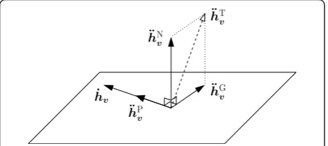
The derivatives of the lifted line ḣ_v and ḧ_v can be interpreted physically: If a point moves along the lifted line hv(m) in the sample space, where m denotes the time, thenḣv andḧv denote the instantaneous velocity and instantaneous accelerationat time m= 0, respec-tively. The acceleration can be decomposed in three parts

v is parallel to the velocity

vector ḣv and, thus, parallel to the tangent plane. It corresponds to the change in velocity of the moving point. h¨N_v is normal to the tangent plane and describes the change in directionof the velocity vector ḣvnormal to the tangent plane._h¨G

v is parallel to the tangent plane

and normal to the velocity vector ḣ_v. It corresponds to the geodesic acceleration and indicates the change in direction of the velocity vector ḣv parallel to the tan-gent plane. Based on these acceleration components, the curvatures of the solution locus at _θ˜₀ can be deter-mined:

is the normal curvature in direction ofvand is called

intrinsic curvatureand

is the tangentialdcurvature in direction ofvand is called

parameter-effects curvature. The curvatures are divided into normal and tangential components since each com-ponent has a different influence on the accuracy of the lin-ear approximation. On the one hand, the intrinsic curvature is an intrinsic property of the solution locus. It only affects the planar assumption. On the other hand, the parameter-effects curvature only influences the uniform coordinate assumption and depends on the specific para-meterization of the problem. Hence, a reparapara-meterization may change the parameter-effects curvature but not the intrinsic curvature. In order to assess the effect of the cur-vatures on inference, they should be normalized. A suita-ble scaling factor is the so-called standard radius ρ=s√P since its squarer2 = s2Pappears on the right hand side in (19) and (20), which describe the confidence regions. Therelative curvaturesare given by the curva-tures (36) and (37) multiplied with the standard radius:

γN

v =KNvρ, (38)

γT

v =KvTρ. (39)

If the relative curvatures are small compared with

1/

&

F1−α

P,N−P for all possible directionsv, then the corre-sponding assumptions are valid. Hence, it is sufficient to determine themaximum relative curvaturese

N_{= max}

(9)

and to compare them to 1/

&

F1−α

P,N−P in order to assess the accuracy of the confidence regions [11]. If the confi-dence region based on the linearization method (19) with the approximate covariance matrix shall be applied, both the planar assumption and the uniform coordinate assumption have to be fulfilled. That means that the maximum relative curvatures ΓN and ΓT have to be

small compared with 1/

&

F1−α

P,N−P. The confidence region based on the likelihood method (20) is more robust since only the planar assumption needs to be ful-filled and only ΓN needs to be small compared with

1/

&

F1−α

P,N−P.

4.2 Analysis of the parameter estimation problem In the following, the parameter estimation problem is analyzed by calculating the maximum relative curvatures and by plotting the confidence regions (19) and (20) for different signal-to-noise ratios (SNRs). The system setup is as follows: A training preamble of lengthKt=256 is

assumed that covers 10% of the data burst of lengthK =

2,560. A pseudo-random sequence of BPSK symbols is used as training. Since this paper concentrates on the positioning part of the proposed joint communication and positioning system, it is sufficient to focus on the channel estimation and to neglect the data detection. A Gaussian pulse shapeg(τ) =gTx(τ)* gRx(τ) ~ exp (–(τ/

Ts)2) is assumed. After receive filtering, the noise

pro-cess is slightly colored, but we have verified that the correlation is negligible with respect to receiver proces-sing. The training sequence is transmitted over the phy-sical channel and at the receiver side channel parameter estimation as suggested in Section 2.2 is performed. For the purpose of curvature analysis, only PSO as described in [16] with I= 50 particles and a maximum number of

T =8,000 iterations is applied for solving the nonlinear metric Ω(θ). PSO delivers the likelihood confidence region automatically as explained in Section 3.3. The approximate co variance matrix is calculated afterward according to (18). A confidence level of 95% is applied

(a=0.05). Since the curvature measures depend on the parameter set θand also on the noise samples, simula-tions are performed for a fixed channel model at differ-ent SNRs. Two differdiffer-ent channel models are assumed: A single-path channel (M= 1) and a two-path channel (M

= 2) with a small excess delay (Δτ2: =τ2-τ1 = 0.81Ts),

both with a memory length L =10. The parameters of the channels are given in Table 1. Furthermore, the maximum relative curvatures ΓN and ΓT for different

SNRs and the value of 1/

&

F0.95

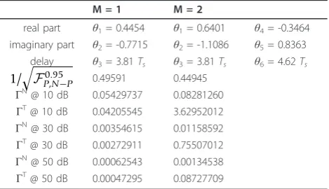
P,N−P are listed in Table 1. It can be concluded that the planar assumption is always

fulfilled sinceΓNis much smaller than 1/

&

F0.95

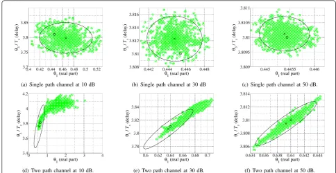
P,N−P in all cases. This means the likelihood method is always accu-rate. For the single-path channel, the uniform coordi-nate assumption is also fulfilled for all SNRs (see Table 1), i.e., the confidence regions based on the linearization method and the approximate covariance matrices are accurate. This is confirmed by Figure 4a, b, c. In Figure 4, the confidence regions based on the linearization method (black ellipse) and the likelihood method (filled dots) are plotted for the parameter combination of the real part θ1 and the delayθ3 of the LOS path

normal-ized with respect to the symbol duration Ts. Both

regions are similar for the single-path channel. In case of the two-path channel, a different situation is observed as shown in Figure 4d, e, f. The uniform coordinate assumption is violated at low SNR sinceΓT isnotmuch

smaller than 1/

&

F0.95

P,N−P (see Table 1). The shape of the likelihood confidence region differs strongly from the ellipse generated by the approximate covariance matrix. Only at high SNR, both shapes coincide. For the two-path channel, the uniform coordinate assumption is valid from approximately 35-40 dB upward. For different channel realizations, different results are obtained. It should be mentioned again that the curvature measures strongly depend on the parameter set θ and on the noise samples. The larger the excess delay Δτ2, the

lower is the nonlinearity of the problem, i.e., the uni-form coordinate assumption is already valid at lower SNR and vice versa. It can be summarized that the con-fidence regions based on the linearization method are not accurate at low SNR in a multipath scenario. Hence, the soft information based on the approximate covar-iance matrix may lead to inaccurate results. The influ-ence of soft information on positioning is investigated in the following section.

Table 1 Parameters of the investigated channel models and the corresponding maximum rel. curvatures at different SNRs

M = 1 M = 2

real part θ1= 0.4454 θ1= 0.6401 θ4= -0.3464

imaginary part θ2= -0.7715 θ2= -1.1086 θ5= 0.8363

delay θ3= 3.81Ts θ3= 3.81Ts θ6= 4.62Ts

1/

&

F0.95

P,N−P 0.49591 0.44945 ΓN

@ 10 dB 0.05429737 0.08281260 ΓT

@ 10 dB 0.04205545 3.62952012 ΓN

@ 30 dB 0.00354615 0.01158592 ΓT

@ 30 dB 0.00272911 0.75507012 ΓN

@ 50 dB 0.00062543 0.00134538 ΓT

(10)

5 Positioning

5.1 Positioning based on the time of arrival

There are many different approaches to determine the position, e.g., multiangulation, multilateration, finger-printing, and motion sensors. This paper focusses on radiolocation based on the TOA, which is also called multilateration. Furthermore, two-dimensional position-ing is considered in the followposition-ing. An extension to three dimensions is straightforward.

The positionp = [x, y]T of a mobile station (MS) is determined relative toBreference objects (ROs) whose positionspb=[xb,yb]T (1≤b ≤ B) are known. For each

ROb, the TOA τ1,ˆ b is estimated. The TOA corresponds to the distance between this RO and the MS rb=τ1,ˆ bc, where cis the speed of light. The estimated distancesr = [r1,...,rB]T are calledpseudo-ranges since they consist

of the true distancesd(p)= [d1(p),..., dB(p)]Tand

esti-mation errors h= [h1,...,hB]T with covariance matrix

r=d(p) +η.:

r=d(p) +η. (42)

The true distance between thebth RO and the MS is a nonlinear function of the positionpgiven by

db(p) =

&

(x−xb)2+ (y−yb)2. (43)

Thus, positioning is again a nonlinear problem.fThere are alternative ways to solve the set of nonlinear equa-tions described by (42) and (43). In this paper, two dif-ferent approaches are considered: The iterative Taylor series algorithm (TSA) [22] and the weighted least-squares (WLS) method [23,24].

The TSA is based on a linearization of the nonlinear function (43). Given a starting position pˆ₀ (initial guess), the pseudo-ranges can be approximated by a first-order Taylor series

r∼= d(ˆp0) +J(ˆp0)(p− ˆp0) +η, (44)

in which J(p) is the Jacobian matrix of (43) with entries

[J(p)]b1=δ

db(p)

δx , [J(p)]b2=

δdb(p)

δy . (45)

Defining r0=r−d(ˆp0) and p0=p− ˆp0 results in

the following linear relationship

r0∼= J(pˆ0)p0+η, (46)

that can be solved according to the least-squares approach:

ˆp0=

J(ˆp0)

T WJ(ˆp0)

−1

J(ˆp0)TWr0. (47)

(a) Single path channel at 10 dB (b) Single path channel at 30 dB (c) Single path channel at 50 dB.

(d) Two path channel at 10 dB. (e) Two path channel at 30 dB. (f) Two path channel at 50 dB.

(11)

The weighting matrixW is given by the inverse of the

covariance matrix Cη :W= diag

1

σ2

η1,. . .,

1

σ2

ηB

. A new

position estimate pˆ₁ is obtained by adding the correc-tion factor ˆp₀ to the starting position pˆ₀. This proce-dure is performed iteratively,

ˆ

p_i₊₁=pˆ_i+ˆp_i, (48)

until the correction factor ˆp_i is smaller than a given threshold. If the initial guess is close to the true posi-tion, few iterations are needed. If the starting position is far from the true position, many iterations may be necessary. Additionally, the algorithm may diverge. Hence, finding a good initial guess is a crucial issue. For the numerical results shown in Section 5.2, the position estimate of the WLS method is used as initial guess for the TSA.

The WLS method [23,24] solves the set of nonlinear equations described by (42) and (43) in closed form. Hence, this method is non-iterative and less costly than the TSA. The basic idea is to transform the original set ofnonlinearequations into a set oflinearequations. For this purpose, one RO is selected as reference. Without loss of generality, the first RO is chosen here. By sub-tracting the squared distance of the first RO from the squared distances of the remaining ROs, a linear least-squares problem with solution

ˆ

p=STWS−1STWb (49)

is obtained, in which

S=

⎡ ⎢ ⎢ ⎢ ⎣

x2−x1y2−y1

x3−x1y3−y1 ..

. ...

xB−x1yB−y1

⎤ ⎥ ⎥ ⎥

⎦ (50)

and

b=−1 2

⎡ ⎢ ⎢ ⎢ ⎣

r2₂−r₁2−R2₂+R2₁ r2₃−r₁2−R2₃+R2₁

.. .

r2

B−r21−R2B+R21

⎤ ⎥ ⎥ ⎥

⎦ (51)

with R2_b =x2_b+y_b2. The weighting matrixW’ is given by:

W= diag

1

σ4

η2,. . .,

1

σ4

ηB

.

Both, the TSA and the WLS method, apply a weight-ing matrix that contains the variances of the pseudo-range errors. Reliable pseudo-pseudo-ranges have higher weights than unreliable ones and, thus, have a stronger influence

on the estimation results. Typically, the true variances are not known. They can only be estimated as described in Section 3: For each linkb, the variance of the TOA

σ2 ˆ

τ1,b is determined via the linearization

g

or the likeli-hood method. This TOA variance is transformed into a pseudo-range variance σ_η2_b by a multiplication withc2. If no information about the estimation errorhis available, the weighting matrices correspond to the identity matrix I(no weighting at all).

The Cramer-Rao lower bound (CRLB) provides a benchmark to assess the performance of the estimators [14]:

CRLB(p) = 2

d=1

[I(p)−1]dd, (52)

where

I(p) =J(p)TWJ(p) (53)

is the Fisher information matrix. If the estimator is unbiased, its mean squared error (MSE) is larger than or equal to the CRLB. If the MSE approaches the CRLB, the estimator is a minimum variance unbiased (MVU) estimator.

The positioning accuracy depends on the geometry between the ROs and the MS and, thus, varies with the position p. This effect is called geometric dilution of precision (GDOP) [22,25]. In order to separate the influ-ence of the geometry from the influinflu-ence of the estima-tion errorshon the positioning accuracy, it is assumed that all pseudo-ranges are affected by the same error variance σ_η2= 1, i.e.,W =I. Given this assumption, the GDOP is the square root of the CRLB:

GDOP(p) ='CRLB(p)|W=I. (54)

5.2 Numerical results

In the following, the overall performance of the pro-posed system concept using soft information is evalu-ated. For this purpose, two scenarios with different GDOP as shown in Figure 5 are considered. The ROs are denoted by black circles and the GDOP is illustrated by contour lines. For both scenarios, B = 4 ROs are located inside a quadratic region with side length√2R, where R = 2Tsc is the distance from every RO to the

(12)

Furthermore, power control is assumed, i.e., the SNR for all links is the same. All results reported throughout this paper are for one-shot measurements.

Three different channel models with memory lengthL =10 are investigated: a single-path channel (M = 1), a two-path channel (M = 2) with large excess delay (Δτ2

Î [Ts,2Ts]) and a two-path channel (M = 2) with small

excess delay (τ2∈[Ts

10,Ts]). For all channel models,

the LOS delay τ1,bfor each link bis calculated from the

true distancedb(p). The excess delay of the multipath

component Δτ2 for both two-path channels is

deter-mined randomly in the corresponding interval. The smaller the excess delay is, the more difficult it is to separate the different propagation paths. The power of the multipath component is half the power of the LOS component. The phase of each component is generated randomly between 0 and 2π. For each link, channel parameter estimation is performed and soft information based on the linearization method and on the likelihood method is obtained. For PSO, I= 50 particles and a maximum number of iterationsT = 8,000 are applied.h

The estimated LOS delays τ1,ˆ b are converted to pseudo-ranges rb, and the position of the MS is estimated with

the TSA and the WLS method applying the different soft information methods. For comparison, positioning without soft information is performed. The position esti-mate of the WLS method is used as initial guess for the TSA. Furthermore, in the WLS method, the RO with the best weighting factor is chosen as reference.

The performance of the estimators is evaluated by Monte Carlo simulations and the results are compared with the Cramer-Rao lower bound (CRLB). On the one hand, simulations are performed over SNR since the accuracy of the soft information methods depends on the SNR. In each run, a new MS position p is deter-mined randomly inside the region of Figure 5. On the other hand, simulations are performed over space for a fixed SNR in order to assess the influence of the GDOP. A fixed 4 × 4 grid of MS positions is applied in this case.

Different channel realizations are generated during the Monte Carlo simulations. Since different channel reali-zations result in different weighting matricesW, a mean CRLB is introduced,

where the expectation is taken with respect to the channel realizations. For the simulations over SNR, the expectation is additionally taken with respect to the ran-dom positionsp.

The simulation results are shown in Figure 6. There are eight different graphs (6a, b, c, d, e, f, g, h) arranged in an array with two columns and four rows. In the first column, the results for the simulations over SNR are shown. The second column contains the results for the simulations over space at 30 dB. In each row, the results for a fixed simulation setup are illustrated. All graphs show the root mean squared error (RMSE) of pˆ nor-malized with respect tods= cTsfor positioning without

soft information ("wo”), with soft information from the likelihood method ("like”), and with soft information from the linearization method ("lin”). The square root of the mean CRLB (normalized with respect to ds), which

is denoted simply as CRLB in the following, is plotted for comparison ("crlb”). Curves labeled with “L” were obtained for the first scenario with large average GDOP, and curves labeled with“S” were obtained for the sec-ond scenario with small average GDOP.

At first, the results for the single-path channel are dis-cussed because this scenario represents an optimal case: Both soft information methods are accurate (see Section 4.2) and due to power control, the pseudo-range errors 2

(a) Scenario with large average GDOP.

1.02

(b) Scenario with small average GDOP.

(13)

0 10 20 30 40 50 60

(a) WLS method for a single path channel.

0

(b) WLS method for a single path channel at 30 dB.

0 10 20 30 40 50 60

(c) TSA for a single path channel.

0

(d) TSA for a single path channel at 30 dB.

0 10 20 30 40 50 60

Figure 6RMSE of pˆ normalized with respect tods= cTsfor positioning without soft information ("wo”), with soft information from the likelihood method ("like”), and with soft information from the linearization method ("lin”). For comparison

&

CRLB(p) normalized

with respect todsis plotted ("crlb”). Curves labled with“L”were obtained for the scenario with large average GDOP, and curves labeled with“S”

were obtained for the scenario with small average GDOP. (a) WLS method for a single-path channel. (b) WLS method for a single-path channel at 30 dB. (c) TSA for a single-path channel. (d) TSA for a single-path channel at 30 dB. (e) TSA for a two-path channel with_Δ_τ2Î[Ts,2Ts]. (f) TSA

for a two-path channel withΔτ2Î[Ts,2Ts] at 30 dB. (g) TSA for a two-path channel with τ2∈[T₁₀s,Ts]. (h) TSA for a two-path channel with

τ2∈[Ts

(14)

for all ROs should be the same. Hence, positioning without and with weighting is supposed to perform equally well. The first row of Figure 6 contains the results for the WLS method, whereas the second row shows the results for the TSA. As supposed previously, the RMSE curves for positioning without soft informa-tion and with soft informainforma-tion from the likelihood and the linearization method coincide. The TSA is further-more a MVU estimator since the RMSE approaches the CRLB for all SNRs and for all positions. The WLS method performs worse: There is a certain gap between the CRLB and the RMSE. In Figure 6b, it can be observed that this gap depends on the position and, thus, on the GDOP: The larger the GDOP is, the larger is the gap. Hence, the gap between RMSE and CRLB in Figure 6a is smaller for the second scenario ("S”) since the GDOP is smaller on average. For the two-path chan-nels, a similar behavior of the WLS method was observed. Therefore, only the results for the TSA are considered in the following due to its superior performance.

The third and fourth row of Figure 6 show the simula-tion results for the two-path channels with large and small excess delay, respectively. It was observed in Sec-tion 4.2 that the likelihood method is generally accurate even for multipath channels. In contrast, the accuracy of the linearization method depends on the excess delay and the SNR. The smaller the excess delay, the higher is the nonlinearity of the problem and the less accurate is the linearization method. The accuracy increases with SNR. Hence, it is supposed that the likelihood method outperforms the linearization method. Only at very high SNR, both methods are assumed to perform equally well. Surprisingly, the linearization and the likelihood method show approximately the same performance for all cases. The linearization method performs even slightly better in most cases. Only for very low SNR and a small excess delay the likelihood method outperforms the linearization method. The likelihood method seems to be more susceptible to the GDOP. Hence, the inaccu-racy of the covariance matrices at low SNR barely influ-ences the positioning accuracy. Actually, it seems that the absolute value of the weights in the weighting matricesWandW’ is not crucial. Rather a correct ratio of the weights is relevant. Thus, rough soft information is sufficient as long as the ratio of the pseudo-range var-iances is accurate. This is fulfilled even for the inaccu-rate covariance matrices of the linearization method. Hence, it is suggested to apply the linearization method because of its lower computational complexity.

For the two-path channel with large excess delay (Fig-ure 6e, f), the RMSE with or without soft information is almost the same since the multipath components can already be separated by the estimator quite well. For a

small excess delay (Figure 6g, h), the RMSE with soft information is much closer to the CRLB than without soft information. With respect to SNR, a gain of approximately 7-10 dB is achieved (see Figure 6g). Furthermore, positioning with soft information is less susceptible to the GDOP (see Figure 6h). Thus, soft information is well suited to mitigate severe multipath propagation. The smaller the excess delay is, the more important it is to apply soft information for positioning.

The influence of the GDOP can be neglected for the scenario with small average GDOP. The curves labeled with“S”indicate that even for one-shotestimation with-out oversampling a positioning accuracy much smaller than the distance corresponding to the symbol duration,

ds, is achieved for all channel models.

For all simulations, a LOS path has been assumed so far. Hence, the estimated TOA corresponds to distance between transmitter and receiver. However, in urban or indoor environments, the LOS path is often blocked as already mentioned in Section 2.1. Therefore, the influ-ence of NLOS propagation is discussed here. In case of NLOS, a modeling error is introduced that reduces the positioning accuracy significantly. The proposed soft channel parameter estimator does not take a priori information about the physical channel (e.g., probability of NLOS) into account and, hence, is not able to detect such a modeling error. The obtained soft information can only be used to mitigate multipath propagation. In order to mitigate NLOS effects, further processing has to be done (e.g., [24]).

Nevertheless, multipath mitigation is an important issue. The multipath mitigation ability of the proposed soft channel parameter estimation has been presented for M =2 paths due to clarity and simplicity reasons. The influence of the number of multipath components is as follows: The complexity of the soft channel para-meter estimator increases with the number of multipath components. Furthermore, the reliability of the estimates decreases withM. Hence, the positioning accuracy dete-riorates. If M is large and the scatterers are closely spaced (dense multipath), the estimator becomes biased and the positioning accuracy saturates. In general, it is suggested to consider only the dominant paths ifM is large.

It was mentioned before that the TSA may diverge. Divergence occurred for large GDOP when the initial guess was far from the true position.i This happened only rarely. The initial guess is determined by the WLS method which is very susceptible to the GDOP. Hence, the starting position may be far away from the true position for large GDOP.

(15)

cases, it converges to a boundary of the search space, such that the premature convergence can be detected (outage). In Figure 7, the outage rates are shown for both two-path channels: The dashed lines (i) and (iii) denote the probability that the delay estimation fails for one RO and the solid lines (ii) and (iv) denote the prob-ability that two or more ROs fail. If the delay estimation fails for one RO, the position of the MS can be deter-mined nevertheless since only three ROs are necessary for positioning in two dimensions. Only if two or more ROs fail, the position estimation fails, too. By adding more ROs, the outage rate for positioning can be decreased to an arbitrary small amount. The outage rates for the two-channel models differ significantly. For the two-path channel with large excess delay (Δτ2Î [Ts,

2Ts]), the outage rates (i) and (ii) are negligible. In

con-trast, the outage rates (iii) and (iv) for the two-path channel with small excess delay (τ2∈[Ts

10,Ts]) are

quite high at low SNR but decrease significantly with increasing SNR. The smaller the excess delay is, the higher is the probability that PSO converges prematurely.

6 Conclusions

In this paper, a channel parameter estimator based on the maximum-likelihood approach is proposed for joint communication and positioning. The parameters of the physical channel (e.g., TOA) and the equivalent discrete-time channel model are estimated jointly. In order to mitigate multipath propagation effects and to improve the positioning accuracy, soft information concerning the parameter estimates is used. Two dif-ferent methods to obtain soft information are pro-posed: The linearization and the likelihood method.

The accuracy of the methods depends on the nonli-nearity of the parameter estimation problem, which is evaluated by the curvature measures of Bates and Watts. It is shown that the likelihood method is always accurate for the parameter estimation problem. The linearization method is only accurate in a single-path channel or at high SNR for a multisingle-path channel. Nevertheless, Monte Carlo simulations for a two-dimensional positioning problem show that this has only very little influence on the positioning. The posi-tioning algorithms that exploit the soft information obtained by the linearization and the likelihood method perform equally well. For severe multipath propagation, the RMSEs for the weighted positioning algorithms are closer to the CRLB than the RMSE of positioning without weighting. A gain of approxi-mately 7-10 dB can be achieved. Hence, multipath propagation effects can be mitigated significantly, even for one-shot estimation without oversampling. Based on these results, it is suggested to apply the lineariza-tion method because of its lower computalineariza-tional complexity.

Endnotes

a

For oversampling with factor Jit follows: T = Ts

J.

b

The mean squared error of the channel estimates ĥl is

reduced in comparison to the mean squared error of the least-squares channel estimates hl , if the number of parameters, 3M, is less than the number of channel coefficients, L + 1, to be estimated. For simulation results please refer to [4].cCapprox corresponds to Vˆ_a in

[11] for a complex-valued problem instead of a real-valued problem.dThe superscriptT, which denotes tan-gential, should not be mistaken for the superscript T, which denotes thetransposeof a matrix.eIn [13] a sim-plified method to determine the maximum relative cur-vatures is introduced based on linear transformations of the coordinates in the parameter and the sample space. This method is neglected here because it is out of the scope of this paper.fIn a two-dimensional TOA scenario at least three ROs are required. For positioning in three dimensions a fourth RO is needed.gFor the linearization method the variance of the TOA corresponds to the 3rd diagonal entry of the approximate covariance matrix Capprox. h Furthermore, channel parameter estimation

was performed for the LMM described in [18] with the true parameters θ as initial guess. Since PSO and the LMM provided approximately the same performance, only PSO is considered here for conciseness.iThe out-liers due to divergence were not considered in the calcu-lation of the RMSE.

0 10 20 30 40 50 60

SNR in dB 0

10 20 30 40

Outage rate in %

(i) (ii) (iii) (iv)

Figure 7Outage rate of PSO in%: (i) one RO fails/(ii) two or more RO fail in the two-path channel withΔτ2Î[Ts, 2Ts], (iii) one RO fails/(iv) two or more ROs fail in the two-path channel with τ2∈[Ts

(16)

Appendix

In the following, the equivalence of the maximum-likeli-hood estimators based on (9) and (10) is shown. First, both metrics are stated in vector/matrix notation. Then, the equivalence of both metrics is proven given the assumptions of Section 2.2. For readability, the termsh = h(θ) and h˜=h(θ˜) are introduced, whereθ denotes the true parameter set and _θ˜ denotes the hypothetical parameter set.

Equivalently, a metric corresponding to (10) can be derived:

As both metrics have to be minimized, it is sufficient to show that

E(θ˜)=c·E(θ˜), (58)

wherec is a constant that scales the metric but does not change the location of the minimum. The expecta-tion of the first metric can also be written as

E(θ˜)=E

For the second metric follows similarly

E

Comparing (59) and (60) shows that (58) is valid with c= _K_t1₋_L.

Competing interests

The authors declare that they have no competing interests.

Received: 30 November 2010 Accepted: 23 November 2011 Published: 23 November 2011

References

1. R Raulefs, S Plass, C Mensing, The where project: combining wireless communications and navigation, inProceedings of 20th Wireless World

Research Forum (WWRF), Ottawa, Canada (2008)

2. K Pahlavan, AH Levesque,Wireless information networks, ch. 13: RF location sensing, Wiley, Hoboken, New Jersey (2005)

3. K Cheung, H So, W-K Ma, Y Chan, A constrained least squares approach to mobile positioning: algorithms and optimality. EURASIP J Appl Signal Process 23 (2006). p (2006) Article ID 20858

4. K Schmeink, R Block, PA Hoeher, Joint channel and parameter estimation for combined communication and navigation using particle swarm optimization, inProceedings of Workshop on Positioning, Navigation and

Communication (WPNC), Dresden, Germany (2010)

5. A Khayrallah, R Ramesh, G Bottomley, D Koilpillai, Improved channel estimation with side information, inProceedings of IEEE Vehicular Technology

Conference (VTC Spring), vol. 2. (Phoenix, Arizona, 1997), pp. 1049–1053

6. JW Liang, B Ng, JT Chen, A Paulraj, GMSK linearization and structured channel estimate for GSM signals, inProceedings of IEEE Military

Communications Conference (MILCOM), vol. 2. (Monterey, California, 1997),

pp. 817–821

(17)

8. M Feder, E Weinstein, Parameter estimation of superimposed signals using the EM algorithm. IEEE Trans Acoust Speech Signal Process.36(4), 477_–489 (1988). doi:10.1109/29.1552

9. BH Fleury, M Tschudin, R Heddergott, D Dalhaus, KI Pedersen, Channel parameter estimation in mobile radio environments using the SAGE algorithm. IEEE J Sel Areas Commun.17(3), 434_–450 (1999). doi:10.1109/ 49.753729

10. A Richter, M Landmann, RS Thomä, Maximum likelihood channel parameter estimation from multidimensional channel sounding measurements, in

Proceedings of IEEE Vehicular Technology Conference (VTC Spring), Jeju, Korea,

pp. 1056–1060 (2003)

11. JR Donaldson, RB Schnabel, Computational experience with confidence regions and confidence intervals for nonlinear least squares, inProceedings

of 17th Symposium on the Interface of Computer Sciences and Statistics,

Lexington, Kentucky, pp. 83_–93 (1985)

12. M Schwaab, EC Biscaia Jr, JL Monteiro, JC Pinto, Nonlinear parameter estimation through particle swarm optimization. Chem Eng Sci.63(6), 1542–1552 (2008). doi:10.1016/j.ces.2007.11.024

13. DM Bates, DG Watts, Relative curvature measures of nonlinearity. J R Stat Soc Ser B (Methodological).42(1), 1–25 (1980)

14. SM Kay,Fundamentals of Statistical Signal Processing: Estimation Theory (Prentice-Hall, Upper Saddle River, New Jersey, 1993)

15. J Kennedy, R Eberhart, Particle swarm optimization, inProceedings of IEEE

International Conference on Neural Networks, vol. 4. Perth, Australia, pp.

1942–1948 (1995)

16. D Bratton, J Kennedy, Defining a standard for particle swarm optimization,

inProceedings of IEEE Swarm Intelligence Symposium (SIS), Honolulu, Hawaii,

pp. 120_–127 (2007)

17. C Blum, X Li, Swarm Intelligence in Optimization, inSwarm Intelligence:

Introduction and Applications, ser. Natural Computing Series, ed. by C Blum,

D Merkle (Springer, 2008), pp. 43–85

18. WH Press, SA Teukolsky, WT Vetterling, BP Flannery,Numerical Recipes in C+

+: The Art of Scientific Computing(Cambridge University Press, Cambridge,

2002)

19. J Nocedal, SJ Wright,Numerical Optimization(Springer, New York, 1983) 20. PA Hoeher, P Robertson, E Offer, T Woerz, The soft-output principle:

reminiscences and new developments. Eur Trans Telecommun.18(8), 829–835 (2007). doi:10.1002/ett.1200

21. JE Dennis Jr, RB Schnabel,Numerical Methods for Unconstrained

Optimization and Nonlinear Equations(Prentice-Hall, Englewood Cliffs, New

Jersey, 1983)

22. ED Kaplan, (ed.),Understanding GPS: Principles and Applications(Artech House, Boston, 1996)

23. AH Sayed, A Tarighat, N Khajenouri, Network-based wireless location: challenges faced in developing techniques for accurate wireless location information. IEEE Signal Process Mag.22(4), 24_–40 (2005)

24. I Guevenc, CC Chong, F Watanabe, H Inamura, NLOS identification and weighted least-squares localization for UWB systems using multi-path channel statistics. EURASIP J Appl Signal Process 1–14 (2008). (2008) Article ID 271984

25. RB Langley, Dilution of precision. GPS World.10(5), 52–59 (1999)

doi:10.1186/1687-1499-2011-185

Cite this article as:Schmeinket al.:Joint communication and positioning based on soft channel parameter estimation.EURASIP Journal on Wireless Communications and Networking20112011:185.