Classification of brain MRI images by comparing SVM classifier and PNN classifier using Confusion Matrix

(1)

IJEDR1601039

International Journal of Engineering Development and Research (www.ijedr.org)

223

Classification of brain MRI images by comparing

SVM classifier and PNN classifier using Confusion

Matrix

1_{Ms. Ashwini J. Sankhe,} 2 _{Prof. S.K.Bhatia}

1_{ME Student, Department of Electronics and Telecommunication, JSPM’s ICOER, Wagholi, Pune,} 2_{Assistant Professor, Department of Electronics and Telecommunication, JSPM’s ICOER, Wagholi, Pune}

1_{Dept. of EXTC, JSPM’s ICOER, Wagholi, Pune}

________________________________________________________________________________________________________ Abstract - Image classification will be used for automated visual inspection to classify MRI images. It will be performed through textures analysis and probabilistic neural network as well as support vector machine. The textures are extracted using co-occurrence features. There are 6 classes of brain MRI having different brain disease. The proposed method contains HARVARD Database contains training and testing images. After feature extraction, confusion matrix is plotted with the help of training data and testing data. Confusion matrix gives accuracy for each class and also gives overall accuracy for support vector machine and probabilistic neural network

IndexTerms - GLCM, Feature Extraction, MRI, Confusion matrix, SVM Classifier, PNN Classifier.

________________________________________________________________________________________________________

I.INTRODUCTION

MRI is a system which has many applications and more than 25,000 scanners are used in worldwide. MRI has an drive on conclusion and treat in many specialties although the effect on better fitness outcomes is provisional. The use of MRI is usually in preferred to CT when either modality could give up the same in sequence as MRI does not require any ionization emission. MRI is in general a secure method but there are number of incidents which harmful to patients. Contraindications to MRI include most cochlear implants and cardiac pacemakers, shrapnel and metallic strange bodies in the eyes. The protection of MRI during the first trimester of pregnancy is unsure, but it may be preferable to other options. The continued amplify in order for MRI inside the healthcare industry has led to concerns about cost efficiency and over conclusion.

MRI is a medical imaging method used in radiology to image the composition and used diagnose to disease. MRI scanners uses high power magnets generate magnetic fields, radio waves, and field gradients to form images of the body. As MRI scanner has tunnel shaped tool which generates sequence of gradient which change magnetic field to its precise level and it also requires cross-sectional area of image. When the RF pulse ceases, the hydrogen ions come back to their inhabitant state and free the energy immersed from the pulses. This low energy (in the pW range) is detected by the recipient coils in the MRI and sent to a computer, where an Inverse Fourier transformation (IFT) converts the indication from the protons as arithmetical (k-space (magnetic resonance imaging)) data into a picture that can be interpreted by the clinician. The method is broadly used for identification and performance of disease and without affecting the human body to ionizing radiation in hospitals.

There are two types of category: Supervised learning technique and unsupervised learning technique. Supervised learning technique contains Artificial Neural Network (ANN), Support Vector Machine (SVM) and K-Nearest Neighbor (KNN) which are used for classification. Unsupervised learning technique contains K-means Clustering, Self Organizing Map (SOM) used for data clustering.

II.SYSTEMDESCRIPTION

(2)

IJEDR1601039

224

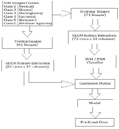
Fig 1 System Architecture

As per the block diagram Fig.1every block describes process of classification of images. Proposed system consist of training phase and testing phase, classification of brain MRI images into different classes. For feature extraction, gray level co-occurance matrix is used. Confusion matrix is used to calculate accuracy of classifier with the accuracy of different brain MRI image classes.

A. Classifier Design:

Classifier design consists of establishing the logical structure of classifier and the mathematical basis of the classification rule. Commonly, for each object encountered, the classifier computes, for each of the classes, a value that indicates (by its magnitude) the degree to which that object resembles the object that are typical of that class. This value is computed as a function of the feature and it is used to select the most appropriate class. Most classifier decision rules reduce to a threshold rule that partitions the measurement space into disjoint region one for each class. If the feature value fall within a particular region, then the object is assigned to the corresponding class.

B. Classifier Training:

Once the basic decision rules of the classifier have been established, one must determine the particular threshold values that separate the classes. This is generally done by training the classifier on a group of known objects. The training set is a collection of objects from each class that have been previously identified by some accurate method. Objects in training set are measured and measurement space is partitioned, by decision surfaces into regions that maximize the accuracy of the classifier when it operates on the training set.

C. Classifier Testing:

A classifier’s accuracy is directly estimated by tabulating its performance on a known test set of object. If the test set is big enough to be representative of objects at large and if it is free of error, the resulting estimate of performance can be quite useful. An alternative method of estimating performance is to use a test set of known objects to estimate PDFs of features for objects belonging to each group. A better approach is to use separate test set for evaluating the performance of classifier.

D. Feature Extraction:

The most important step in abnormality detection is the ability of extracting some unique attributes from MRI image, which help to generate a specific code for each individual. Therefore, feature extraction is a crucial step to the success of an classification system. In order to provide accurate classification of brain MRI images, the most discriminating information present in an MRI image must be extracted. Only the significant features of the image must be encoded so that comparisons between templates can be made.

Features, the characteristics of the objects of interest, if selected carefully are representative of the maximum relevant information that the image has to offer for a complete characterization of a lesion.

E. Gray Level Co-occurance Matrix (GLCM)

A co-occurrence matrix is also known as a co-occurrence distribution. It is defined over an image to be the distribution of co-occurring values at a particular offset.Originally it was proposed by R.M. Haralick, the co-occurrence matrix representation of texture features explores the grey level spatial dependence of texture. A mathematical definition of the co-occurrence matrix is as follows:

- Given a position operator P(i,j), - Let Abe an n x n matrix

- Whose element A[i][j] is the number of times that points with grey level (intensity) g[i] occur, in the position specified by P, relative to points with grey level g[j].

(3)

IJEDR1601039

225

- C is called a co-occurrence matrix defined by P.

Examples for the operator P are: “i above j”, or “i one position to the right and two below j”, etc.

For example; with an 8 grey-level image representation and a vector t that considers only one neighbor, we would find:

1 1 5 6 8

2 3 5 7 1

4 5 7 1 2

8 5 1 2 5

Fig 2: Image example

GLCM is formed from gray scale image. Therefore we want to convert the color image into gray scale image by using MATLAB. The GLCM is calculates how regularly a pixel with gray-level i.e. grayscale intensity or Tone value i occurs either horizontally, vertically, or diagonally to adjacent pixels with the value j. The directions are analyzed according to directions. The directions are mentioned by using angle. For example horizontal direction is mentioned by 0ᴼ, vertical direction is represented by 90ᴼ, bottom left to top right diagonal is represented by -45ᴼ and top left to bottom right is represented by -135ᴼ. It is denoted by P0, P90, P45 and P135.

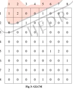
Now for image above we will take horizontal approach. The given image has gray level values form 1 to 8. So the gray level co-occurrence matrix (GLCM) should be of dimension 8×8. Now the pixel value 1 having a pixel valued 2 immediately right to it is occurred two times in the image. Therefore in gray level co-occurrence matrix the value of element (1, 2) is 2. Similarly for the pixel value 1 having a pixel valued 1 immediately right to it is occurred only one time in the image so value of element (1, 1) is 1. Value of (5, 7) is 2, value of (1, 5) is 1, value of (2,3) is 1, value of (2,5) is 1, value of (3,5) is 1, value of (4,5) is 1, value of (5,1) is 1 , value of (5,6) is 1, value of (5,7) is 2, value of (6,8) is 1, value of (7,1) is 2, value of (8,5) is 1. All other elements of GLCM (gray level co-occurrence matrix) are 0.This way we can find the gray level co-occurrence matrix (GLCM).

Fig 3: GLCM G. Support Vector Machine:

A supervised machine learning technique supports classification easily and accurately. In this paper multi-class SVM was applied based on the best features available in the reduced dimensions of template to upgrade the performance ratio. Multi-

1

2

3

4

5

6

7

8

1

2

0

1

0

2

0

1

0

1

0

3

0

1

0

4

0

1

0

5

1

0

1

2

0

6

0

1

7

2

0

(4)

IJEDR1601039

226

class SVM generated 40 classes separately for authorized users. Sample of multi-class SVM is depicted. Selecting a specific kernel and parameters are usually done in a try-and-see manner. SVM classifier’s retrieved data from the template was generated in feature extraction stage. It draws the hyper plane to classify the given data.

Machine Learning is ability to enable the computer to learn. It uses algorithm and techniques which perform different tasks and activities to provide efficient learning. Our main problem is that how can we represent complex patterns and how to exclude bogus patterns. Support Vector Machine is a machine learning tool used for classification and regression. Support Vector Machine is based on supervised learning which classifies points to one of two disjoint half-spaces. It uses nonlinear mapping to convert the original data into higher dimension. Its objective is to construct a function which will correctly predict the class to which the new point belongs and the old points belong. With an appropriate nonlinear mapping, two data sets can always be divided by hyperplane. Hyperplane separates the tuples of one class from another and defines decision boundary. There are many hyper planes that separate the data but only one will achieve maximum separation. The main reason behind maximum margin or separation because if we use a decision boundary to classify, it may end up nearer to one set of datasets compared to others. This was the case when data is linear but mostly we find data is non-linear and data set is inseparable then we use kernels. The core purpose of SVM is to separate the data with decision boundary and extends it to non-linear boundaries using kernel trick. Major benefit of Svm is versatile means different Kernel functions can be specified for the decision function. General kernels are provided, but it is also possible to specify custom kernels.

SVM becomes prominent when we used pixel maps as input; it gives accuracy equivalent to neural networks with elaborated features in a handwriting recognition task. Support vector machine is used for many applications such as text categorization, pattern recognition, face recognition, handwriting analysis but especially for classification and regression applications. Neural Networks are easier to apply than support vector machine but sometimes it provides insufficient results. Even the perceptron learning algorithms (e.g. gradient descent) are slower than SVM learning. Svm has been found to be unbeaten when used for pattern classification problems. One of the major challenge is that of choosing a suitable kernel for given application. But there are many standard or default choices such as Gaussian or polynomial kernel but if these prove worthless then more elaborate kernels are needed. Traditional Classification approaches perform weakly when working directly because of high dimensionality of data but support vector machine can avoid the pitfalls of very high dimensionality representations. Support vector machine is the most promising technique and approach as compared to others. Support vector machine scales fairly well to high dimensional data and the trade-off between classifier complexity and error can be controlled explicitly. Another benefit of SVMs and kernel methods is that one can design and use a kernel for a particular problem that could be applied directly to the data without the need for a feature extraction process. It is particularly important in problems where a lot of structure of the data is lost by the feature extraction process. Example is text processing. Limitations of Svm are speed, size both in training and testing. Discrete data presents another problem. Most severe difficulty with SVMs is the high algorithmic complexity and extensive memory requirements. In short we can say that the development of SVM is an utterly different from standard algorithms used for learning and SVM provides a fresh insight into this learning.

H. Probabilistic Neural Network:

A probabilistic neural network is predominantly a classifier.PNN uses a supervised training set to develop probability density functions within a pattern layer. This is a model based on competitive learning with a ‘winner takes all attitude’ and the core concept based on multivariate probability estimation. Probabilistic (PNN) and General Regression Neural Networks (GRNN) have similar architectures, but there is a fundamental difference. Probabilistic networks perform classification where the target variable is categorical, whereas general regression neural networks perform regression where the target variable is continuous. If you select a PNN/GRNN network, DTREG will automatically select the correct type of network based on the type of target variable.

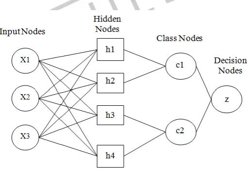
Fig 4: Architecture of PNN

All PNN networks have four layers:

(5)

IJEDR1601039

227

standardize the range of the values by subtracting the median and dividing by the interquartile range. The input neurons then feed the values to each of the neurons in the hidden layer.

ii. Hidden layer: - This layer has one neuron for each case in the training data set. The neuron stores the values of the predictor variables for the case along with the target value. When presented with the x vector of input values from the input layer, a hidden neuron computes the Euclidean distance of the test case from the neuron’s center point and then applies the RBF kernel function using the sigma value(s). The resulting value is passed to the neurons in the pattern layer.

iii. Pattern layer / Summation layer: - The next layer in the network is different for PNN networks and for GRNN networks. For PNN networks there is one pattern neuron for each category of the target variable. The actual target category of each training case is stored with each hidden neuron; the weighted value coming out of a hidden neuron is fed only to the pattern neuron that corresponds to the hidden neuron’s category. The pattern neurons add the values for the class they represent (hence, it is a weighted vote for that category).

iv. Decision layer

: - The decision layer is different for PNN and GRNN networks. For PNN networks, the decision layer

compares the weighted votes for each target category accumulated in the pattern layer and uses the largest vote to predict the target category.

I. Confusion Matrix:

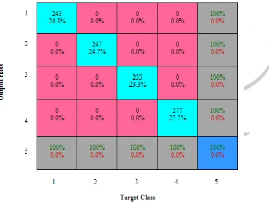
Confusion matrix has two classes, target class and output class. This matrix is used for multiple classifications. Confusion matrix is also called as contingency matrix for supervised learning and for unsupervised learning; it is called as matching matrix.

For confusion matrix plot, the rows shows target class and columns shows output class. Matching of target class and output class is shown in diagonal cell. The off diagonal cells show class which are not matching. The right side column shows output class accuracy and bottom row shows target class accuracy. The overall accuracy shown at bottom right of cell.

Fig 5: Confusion Matrix

III.SIMULAEDRESULTS:

The normal and defective types of images are shown below. Images of brain MRI diseases are taken.

(6)

IJEDR1601039

228

(a) Glioma (b) Meningioma (c) Sarcoma (d) Alzheimer (e) Agnosia

Fig 7: Examples of Different types of disease of brain

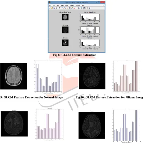
HARVARD database contains different classes of MRI images. Database contains training images and testing images. Gray Level Co-occurance Matrix is used to extract the features. Following figure shows GLCM Feature Extraction for 3 classes i.e. Normal, Sarcoma and Alzheimer disease. The graph shows number of extracted features.

Fig 8: GLCM Feature Extraction

Fig 9: GLCM Feature Extraction for Normal Image

Fig 10: GLCM Feature Extraction for Glioma Image

(7)

IJEDR1601039

229

Fig 13: GLCM Feature Extraction for Alzheimer Image Fig 14: GLCM Feature Extraction for Agnosia Image

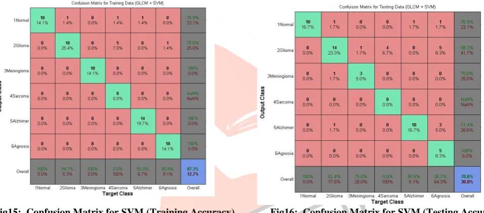
After feature extraction using Gray level co-occurance matrix, confusion matrix for SVM classifier with training and testing data (GLCM + SVM) is done. In confusion matrix, target class vs output class is plotted. The diagonal cell shows where target class and output class match. Overall accuracy is shown at last row of plot which. Each class gives different overall accuracy.

Fig15: Confusion Matrix for SVM (Training Accuracy) Fig16: Confusion Matrix for SVM (Testing Accuracy)

Confusion matrix for Support vector Machine is plotted. For Support vector machine, training accuracy and testing accuracy is calculated. We get 87.3% Training Accuracy and 70% Testing Accuracy for Support Vector Machine.

For comparing SVM classifier with PNN classifier, Confusion matrix for PNN classifier is also calculated. Also for Probabilistic Neural Network, training accuracy and testing accuracy is calculated. We get 100% Training Accuracy and 96.7% Testing Accuracy for Probabilistic Neural Network.

(8)

IJEDR1601039

230

All four confusion matrix gives comparison between SVM classifier and PNN classifier. From above four results, PNN classifier get more accuracy than SVM classifier which means that PNN classifier is more accurate than SVM classifier.Confusion matrix gives clear difference in accuracy of SVM classifier and PNN classifier.

The following table shows difference in training and testing accuracy for SVM classifer and PNN classifier.

TABLE 6.1 Comparison of Testing Accuracy of SVM and PNN Sr.

No. Class

Accuracy (SVM) Accuracy (PNN) Overall TRAINING Accuracy (SVM) Overall TRAINNG Accuracy (PNN)

1 Normal 14.10% 14.10%

87.3% 100%

2 Glioma 25.4% 26.80%

3 Meningioma 14.1% 14.10%

4 Sarcoma 0% 8.50%

5 Alzheimer 19.7% 21.1%

6 Agnosia 14.1% 15.50%

TABLE 6.2 Comparison of Training Accuracy of SVM and PNN

IV.CONCLUSION

In this work, classification of brain MRI images by comparing SVM classifier and PNN classifier gives rise to increase in training and testing speed of feature extraction. This proposed system provides better accuracy for PNN classifier than SVM classifier.

As per results PNN classification gives more efficient results as it takes less time to calculate accuracy whereas SVM classifier takes more time to calculate accuracy. Our proposed method gives graph of number of feature extracted from gray level co-occurance matrix. PNN classification gives more reliable and accurate result.

REFERENCES

[1] Turid Torheim, Eirik Malinen, Knut, Kvaal, Heidi Lyng, Ulf G. Indahl, Erlend K. F. Andersen, Cecilia M. Futsether, “Classification of Dynamic Contrast Enhanced MR Images of Carvical Cancers Using texture analysis and support vector machine” IEEE Trans. medical imaging, vol. 33, NO.8, august 2014

[2] T. Song, M. Jamshidi, R.R. Lee, M. Huang, “A modified probabilistic neural network for partial volume segmentation in brain MR image,” IEEE Trans.on neural network., vol. 18, no. 5, pp. 1424–1432, Sep. 2007

[3] D.F. Specht, ―Probabilistic Neural Networks for Classification, mapping, or associative memory‖, Proceedings of IEEE International Conference on Neural Networks, Vol.1, IEEE Press, New York, pp. 525-532, June 1988

[4] E. Chen, P. Chung, C.L. Chen, H.M. Tsai, C. Chang, “An automatic diagnostic system for CT liver image classification” IEEE trans. On Biomedical Engineering., vol. 45, no. 6, Jul. 1998.

[5] JieTian, ShanhuaXue, Haining Huang, “Classification of Underwater Objects Based on Probabilistic Neural Network”, 2009 Fifth International Conference on Natural Computation,pp.38-42

[6] Daljit Singh, and KamaljeetKaur, Classification of Abnormalities in Brain MRI Images Using GLCM, PCA and SVM , International Journal of Engineering and Advanced Technology (IJEAT)2012,ISSN: 2249 – 8958, Volume-1, Issue-6. [7] Lalit P. Bhaiya and Virendra Kumar Verma, Classification of MRI Brain Images Using Neural Network, International

Journal of Engineering Research and Applications (IJERA) 2012, ISSN: 2248-9622 www.ijera.com

[8] Zacharaki E.I., Sumei Wang, Chawala S., Dong Soo Yoo, Wolf R., Melhem E.R., DavatzikosC., “MRI based classification of brain tumour type and grade using SVM-REF,” IEEE International Symposium on Biomedica Imaging, July 2009, pp. 1035-1038.

[9] Jin Liu, Min Li, Jianxin Wang , Fangxiang Wu, Tianming Liu, and Yi Pan,“ASurvey of MRI-Based Brain Tumor Segmentation Methods” IEEE Conference.TSINGHUA SCIENCE AND TECHNOLOGY, vol. 319, no. 6, pp. 578–595, Dec 2014.

[10] Othman M.F.B., Abdullah N.B., Kamal N.F.B., "MRI brain classification using support vector machine,"International conference on modeling, simulations and applied optimization, pp. 1-4, April 2011.

Sr.

No. Class

Accuracy (SVM)

Accuracy (PNN)

Overall TESTING Accuracy (SVM)

Overall TESTING Accuracy (PNN)

1 Normal 16.70% 16.70%

70% 96.7%

2 Glioma 23.3% 28.3%

3 Meningioma 5% 6.70%

4 Sarcoma 0% 5%

5 Alzheimer 16.70% 18.3%