Copyright2001 by the Genetics Society of America
Enhanced Efficiency of Quantitative Trait Loci Mapping Analysis Based on
Multivariate Complexes of Quantitative Traits
Abraham B. Korol, Yefim I. Ronin, Alexander M. Itskovich, Junhua Peng and Eviatar Nevo
Institute of Evolution, University of Haifa, Haifa 31905, Israel Manuscript received February 20, 2000
Accepted for publication January 10, 2001
ABSTRACT
An approach to increase the efficiency of mapping quantitative trait loci (QTL) was proposed earlier by the authors on the basis of bivariate analysis of correlated traits. The power of QTL detection using the log-likelihood ratio (LOD scores) grows proportionally to the broad sense heritability. We found that this relationship holds also for correlated traits, so that an increased bivariate heritability implicates a higher LOD score, higher detection power, and better mapping resolution. However, the increased number of parameters to be estimated complicates the application of this approach when a large number of traits are considered simultaneously. Here we present a multivariate generalization of our previous two-trait QTL analysis. The proposed multivariate analogue of QTL contribution to the broad-sense heritability based on interval-specific calculation of eigenvalues and eigenvectors of the residual covariance matrix allows prediction of the expected QTL detection power and mapping resolution for any subset of the initial multivariate trait complex. Permutation technique allows chromosome-wise testing of significance for the whole trait complex and the significance of the contribution of individual traits owing to: (a) their correlation with other traits, (b) dependence on the chromosome in question, and (c) both a and b. An example of application of the proposed method on a real data set of 11 traits from an experiment performed on an F2/F3 mapping population of tetraploid wheat (Triticum durum ⫻ T. dicoccoides) is provided.
T
HE detection power and mapping resolution of Soller1994), replicated progeny testing (Sollerand Beckmann 1990), and sequential experimentation marker analysis of quantitative traits are the majorfactors affecting practical applications of quantitative (MotroandSoller1993). For example, in composite mapping the increase in mapping resolution derives trait loci (QTL) mapping. These characteristics strongly
depend on the effect of the QTL in question relative from a reduction of the residual variation by taking into account the effects of cosegregating QTL.
to the phenotypic variance of the trait in the mapping
population. The higher the discrepancy between QTL In QTL mapping, the experimental design usually includes simultaneous measurements of many related groups (or the contribution of the QTL to the trait
heritability H2, the proportion of genetic variation2
G and unrelated quantitative traits and subsequent treat-ment of the individual traits. Recently, several groups in total phenotypic variation2
Phof the trait) the better
the expected QTL detection power and mapping resolu- attempted to improve the efficiency of marker analysis of QTL by taking into account possible effects of the tion. As shown by Landerand Botstein (1989), the
expected value of the log-likelihood test statistics in- putative QTL on several traits simultaneously (Korol
et al.1987, 1995, 1998a;Amoset al.1990;Schorket al.
creases monotonically withH2:
1994; Jiangand Zeng 1995; Ronin et al. 1995, 1998, ELOD⫽ ⫺1⁄2Nlog(1⫺H2). (1)
1999;Welleret al.1996;Almasyet al.1997;Boomsma andDolan 1998; Manginet al. 1998;Henshall and Several strategies have been proposed to improve the
precision of QTL mapping. These involve development Goddard1999;Olsonet al.1999;Williamset al.1999; Zenget al.2000). In the simplest case of two noncorre-of (i) new experimental designs to suit specific mapping
lated traits, the advantage of joint analysis is in the in-goals and an organism’s breeding system, and (ii) new
crease of the multivariate effect according to d2 ⫽ (dx/ QTL mapping models and algorithms to extract
maxi-x)2 ⫹ (dy/y)2 (Figure 1a), where d
x and dy are the mum information about QTL locations and effects. One
substitution effects of the QTL for traitsx andy, and of the improvements includes multilocus (composite)
x and y are the corresponding standard deviations mapping analysis (JansenandStam1994;Zeng1994),
within the QTL groups (residual standard deviations). selective sampling (Lebowitzet al.1987;Darvasiand
Consequently, for a population with 1:1 ratio of the alternative QTL groups (like backcross, dihaploid, or recombinant inbreds) the bivariate analogue of H2
Corresponding author:Abraham Korol, Institute of Evolution,
Univer-sity of Haifa, Haifa 31905, Israel. E-mail: [email protected] could be represented in the form
Figure 1.—The main sources for improvement of QTL mapping efficiency in mul-tiple-trait analysis: (a) due to the pleiotropic effects; (b) due to correlation between the traits (within the QTL groups) caused by nongenetic effects and segregation of unlinked QTL; or (c) due tocombined ef-fectof both foregoing factors.
notype into a one-dimensional phenotype. For the new
H2 xy⫽
1⁄ 4d2
1⫹ 1⁄4d2. (2) phenotype, a higher ratio of the between-QTL group difference to the residual variation can be achieved ow-The situation becomes more complicated when corre- ing to the pleiotropic effect of the QTL on both traits, lated traits are involved. It can be shown (Korolet al. and residual correlation between the traits caused by
1995) that Equation 1 remains valid in bivariate analysis nongenetic factors and segregation at other QTL. These of correlated traits, expectations, illustrated geometrically in Figure 1, are
confirmed by both Monte Carlo simulations and analyti-ELOD(x,y)⫽ ⫺1⁄2N log(1⫺ H2xy) (1⬘)
cal approximations, for marker and interval analysis
with (Korol et al. 1995, 1998a; Ronin et al. 1995, 1999).
Although the described approach resembles the
princi-H2
xy⫽1⫺
2
x2y(1⫺R2xy)
(2
x⫹1⁄4d2x)(2y⫹1⁄4d2y)⫺ 2x2y[Rxy⫹dxdy/(4xy)]2
.
pal component analysis (PCA), it differs from PCA sig-nificantly. Besides technical differences, the main dis-(3)
similarity is that our trait transformations are interval dependent (Korol et al. 1995), whereas in PCA the It was shown earlier that either ELOD(x,y)ⱖELOD(x)
transformation is applied to the initial trait complex and ELOD(x,y)ⱖELOD(y) follow fromH2
xyⱖH2xand
(Welleret al.1996). This difference may be important
H2
xyⱖ H2y, respectively (Korolet al. 1995;Roninet al.
if the mapping population segregates for more than 1999). Given fixeddx/xorH2x ⫽1⁄4d2x/(1⁄4d2x⫹ 2x), how
one QTL (see below). will the resolution be affected by other traits being taken
Clearly, not only statistical reasons are of interest into account? Several situations should be considered
when discussing the advantages of the joint analysis of to explain the expected gain of joint analysis of multiple
correlated trait complexes. The multitrait approach traits compared to single-trait analysis. For the sake of
allows for an integral evaluation of the effects of geno-simplicity, let us consider two traits. As mentioned
mic segments on a defined group of traits. Because of above, ifRxy⫽0, the effect of an additional trait is simply
the internal balance of the organism’s systems ( Schmal-due to the increased Euclidean distance between the
hausen 1942), such an approach for QTL mapping (two-dimensional) centers of the QTL groups (see
Fig-seems to be much more justified biologically than the ure 1a). Consider now the situation when the traits are
usual “trait-by-trait” analysis. It may assist in testing nu-correlated within each of the QTL groups with residual
merous biologically important hypotheses concerning correlation Rxy ⬆ 0. It is easy to see from Equation 3
manifold effects of genomic segments on quantitative that if dy ⬆ 0 and Rxy ⬆ 0 and sign(Rxydxdy) ⬍ 0, then
variation, to distinguish between linkage and pleiotropy
H2
xyⱖH2xand one could expect a respective increase in
as mechanisms of genetic correlation, to address the ELOD. Moreover, the inequalityH2
xy ⬎ H2x holds even
problem of QTL-by-environment interaction, etc. (Korol ifdy⫽0 butRxy⬆0, independent of the sign of
correla-et al.1994, 1998b; JiangandZeng1995;Lebreton et
tion (Figure 1b). Therefore, we can further assume that
al. 1998; Ronin et al. 1999). Such analysis may be of the increment inH2xy, compared withH2x, will result in
major importance in formulating marker-assisted breed-an increased resolution of the mapping breed-analysis (in spite
ing strategies, dissecting heterosis as a multilocus of complications due to certain statistical
nonequiva-multitrait phenomenon, developing optimized pro-lence), no matter how this increment in H2
xy was
pro-grams for evaluation and bioconservation of genetic duced, due to (i) the pleiotropic effect of the QTL on
resources, and revealing the genetic architecture of
fit-xandy, (ii) residual correlation betweenxandy(within
ness systems in natural populations and of multifactorial the QTL groups) caused by nongenetic effects or
segre-diseases in humans. gation of unlinked QTL, or (iii) the combined effect of
The increased number of parameters to be estimated both factors (i) and (ii) (Figure 1c). In other words,
complicates the application of this approach when a instead of separate analyses of traits x andy, one can
large number of traits are considered. Withn traits to conduct joint analysis of these traits that is formally
backcross (as well as a dihaploid or recombinant inbred Roninet al.1995, 1998, 1999; see alsoJiangandZeng 1995) and the foregoing PCA-based models lies in the lines) mapping population using single-interval
map-ping, the model should include (n2⫹5n⫹2)/2 param- fact that the residual variance-covariance matrix was considered interval dependent, in the following sense. eters [QTL position,nmean values,neffects,nresidual
variances, andn(n⫺1)/2 covariances]. Atn⫽10, this Its elements are a subset of the vector of unknown pa-rameters to be estimated by the employed procedure amounts to 76 parameters.
One possible ad hoc simplification of the estimation for each interval, so that for QTL residing in different genomic segments the resulting (transformed) traits aspects is based on a reduction to two-trait analysis
(Korolet al.1995, 1998a;Roninet al.1995, 1999;Jiang could be very different. This interval dependence re-mains a notable characteristic of our new multivariate andZeng 1995) that appeared to be very efficient in
allowing for an increase in QTL detection power and algorithm. mapping resolution. In specific situations, such a
reduc-tion to a two-trait analysis may also be justified by the
THE PROPOSED METHOD biological nature of the involved traits. However, in real
multitrait situations this approach may result in statisti- The model:Assume first that only one QTL segregates cal difficulties caused by the large number of trait pairs. in the mapping population. Consider the genomic seg-Corresponding multiple tests may be interdependent, ment carrying this QTL (with allelesQandq) flanked causing a further complication in defining the critical by markersM
1/m1andM2/m2, with recombination rates values of the test statistics. Another possibility is related r
1 and r2 in intervals M1/m1–Q/qand Q/q–M2/m2. On to the attempt at space transformation, e.g., using the the basis of the marker scores and the measurements PCA (Welleret al.1996;Manginet al.1998) applied of the trait complexx⫽(x
1,x2, . . . ,xn), we should test to the multivariate trait distribution across the entire whether or not variation of any trait ofxindeed depends data set. Although this approach seems to be very attrac- on the interval M1/m1–M2/m
2 and identify the corre-tive, it cannot directly solve the problem when the map- sponding locus Q/q. The expected joint distributions ping population segregates for more than one QTL, of the traits x in each of the marker groups, U
m1m2⫽ especially if some of the effects are relatively strong. U1(x), U
M1m2(x) ⫽ U2(x), Um1M2(x) ⫽ U3(x), and Indeed, assume that in such a case the PCA transforma- U
M1M2(x)⫽ U4(x), can be written as tion was applied to the initial trait complex (without
Ui(x)⫽ ifqq(x)⫹ (1⫺ i)fQq(x), i⫽ 1, . . . , 4, taking out the effects of the target QTL), i.e., for all
individuals independent of their genotypes. Then, the
where the proportions i ⫽ i(r1, r2) depend on un-independence of the resulting derivative traits over the
known recombination ratesr1andr2and mode of inter-entire mapping population cannot guarantee their
in-ference. The specification of then-dimensional densi-dependence within the alternative QTL groups.
More-tiesfqq(x) andfQq(x) depends on the assumptions made over, this problem may exist even in the case of one
about the genetic control of the traits. The simplest case QTL segregating in the mapping population, because
of additive control can be represented by the model the total (across all individuals) variance-covariance
ma-trix of the initial trait complex may differ from the re- x⫽m⫹0.5dgq⫹e, sidual one (i.e., for the matrix characterizing the
within-wherex⫽(x1, . . . ,xn) is the vector of phenotype scores QTL group variation). It is noteworthy that the largest
for an arbitrary individual,e⫽ (e2, . . . ,en) is a vector principal components may be irrelevant in such an
anal-of random variables that obey multivariate normal distri-ysis, as can be seen from Figure 1c (see alsoOlsonet
bution with zero expectations for all coordinates and
al.1999). Nevertheless, in some cases this approach may
(residual) variance-covariance matrixRR⫽{sij},mis the work (in situations represented by Figure 1a).
vector of trait means,d is the vector of the effects of Here we present a generalization of our previous
two-substitution at theQ/qlocus with respect to mean values and three-trait QTL mapping algorithm (Korolet al.
of x, i.e., dxi ⫽ xi(Qq)⫺ xi(qq), and gq denotes the 1995;Roninet al.1995), which is free of the mentioned
genotype at locusQ/q(gq⫽ ⫺1 forqqand 1 for Qq). difficulties, to multivariate trait complexes that allow
Expected improvement owing to multiple-trait
analy-analysis of a large number of traits. It is based on
trans-sis:As in the bivariate case, the QTL detection power formation of the initial trait space into a space of a lower
should depend on the total contribution of the QTL to dimension. In the simplest case of a single-QTL analysis
multivariate phenotypic variation (VPh) of the correlated of a backcross (dihaploid) mapping population, the
trait complex. IfVRis the multivariate residual variation resulting space is one-dimensional independent of the
(within the QTL groups) andVGis the combined be-number of traits, whereas two-QTL analysis for such a
tween-QTL-group discrepancy, then population will employ a two-dimensional model (for
F2 these will be three- and eight-dimensional models, H2
T ⫽VG/VPh⫽VG/(VG⫹VR). (4) correspondingly). The main difference between our
due to the “Euclidean effect,” which grows with the These are (a) to consider the general variance-covari-ance matrix of the traits, which differs from RRdue to number of traits:
the contribution of both QTL (the higher the individual effects of Q1/q1and Q2/q2, the higher the difference);
H2 Eu⫽
1⁄
4
兺
(di/i)21⫹ 1⁄4
兺
(di/i)2. (5)and (b) to consider the residual variation for each QTL as a combined result of nongenetic variation and the Clearly, in the general case of correlated traits, the pure
contribution of all other QTL excluding the one under Euclidean contribution is only a part of the total effect,
consideration. The second possibility provides a rele-so that H2
Eu⬍ H2T. Note that an analogue of Equation vant description of the residual variation for each QTL. 5 can be obtained by canonical transformation of the
Two different approximated procedures, giving very initial trait space (with the within-group covariance
ma-similar results, were employed to implement this ap-trix associated with the QTL under consideration), proach. In both, the LOD score serves as the major allowing the evaluation of the total effect as defined by criterion in interval mapping; the steps of evaluating Equation 4. Then, the multivariate effect of the QTL the QTL effects and QTL position are separated. Both will be manifested as in Equation 5, but with relative are based on our earlier maximum-likelihood approach effects (di/i) in the new coordinate system. Moreover, (Korolet al.1995). Although the proposed procedures using scale transformationsx⬘i ⫽xi/iand correspond- are only approximations of the full procedure, their ing angular transformations, one can map the multivari- major advantage is that they allow treatment of a large ate space into another multivariate space where the number of traits simultaneously.
QTL affects only one trait, withH2
D ⫽ 1⁄4D2/(1⫹ 1⁄4D2) Procedure 1: For each interval, a five-step procedure is being equal to the total contribution of the QTL, as in conducted.
Equation 4 (where Dis the total multivariate effect of
1. The vector of mean trait values in alternative QTL the QTL).
groups defined by flanking markersM1M2andm1m2 The short review in the Introduction indicates that
is evaluated. correlation between traits may be no less (if not more)
2. The same groups are used to define the elements of an important factor affecting the detection power of
the residual (for the currentith interval) covariance multitrait QTL analysis. Therefore, it is of great interest
matrix, RRi. Throughout this article, we assume no to evaluate the contribution of correlations between the
variance-covariance effect (but seeKorolet al.1995, traits toH2
Tin Equation 4. Consequently, in the
follow-1996a), so that RR(QQ) ⫽ RR(qq) and RRi(QQ) ⫽ ing illustrations, we present the expected improvement
RRi(qq). due to the Euclidean effect and the additional
contribu-3. Transformation of the trait space, as described ear-tion due to correlaear-tions. Moreover, although no effect
lier, reduces the problem to a single-trait analysis. is expected from correlations if all effectsdiare 0,
situa-This step includes solving the problem of eigenvalues tions are possible where for only a small subset of traits
and eigenvectors of matrixRRfollowed by scale and
di ⬆ 0, the remaining traits are still very informative
angular transformations, resulting in a new space because of their correlations to the foregoing traits (the
with all effects being absorbed by only one variable simplest such example is provided in Figure 1b).
(“integral” trait; see alsoAllisonet al.1998).
The numerical procedures of interval analysis: The
4. For the resulting variable, a single-trait analysis is distinctive feature of our analysis is that all the
multivari-conducted, with the likelihood function being de-ate transformations are interval-specific (as can be seen
pendent on four parameters, ⫽(,D,,r), where from procedures 1 and 2 described below; see also
, D,, andrstand for the mean value of the new Korolet al.1987, 1995, 1998a; JiangandZeng1995;
trait, total substitution effect, residual standard varia-Ronin et al. 1998), in contrast to the aforementioned
tion, and recombination rate from the left marker, attempts based on canonical transformation applied to
respectively. the entire mixed distribution (Welleret al.1996;
Man-5. After getting the estimates, back transformations can ginet al.1998). To explain why this is important, let us
be conducted, making it possible to get more precise consider the simplest situation with a mapping
popula-estimates of mean values of the QTL groups. Conse-tion polymorphic for two unlinked QTL, sayQ1/q1and
quently, the analysis could be repeated from step (2)
Q2/q2. A double haploid (or recombinant inbred,
back-until a convergent result is obtained. cross, etc.) population will consist of four groups, such
as Q1Q1Q2Q2, Q1Q1q2q2, q1q1Q2Q2, and q1q1q2q2. Assume Procedure 2:This is a simplified version of procedure that the residual (nongenetic) multitrait variation is the
one. It includes three steps and gives approximated same in all four groups and can be described by a vari- results compared with those of procedure 1. However, ance-covariance matrixRR. the differences appear to be very small. For each
inter-Two possibilities for incorporating the joint variation val, the three-step analysis is conducted. of the traits exist when single-QTL mapping analysis is
groups defined by flanking markersM1M2andm1m2 the contribution of different factors to the detection power and mapping resolution of multivariate QTL is evaluated.
2. The same groups are used to define the elements of mapping, a series of variants were simulated that differ with respect to the number of traits (from 1 to 10), the the residual (for the currentith interval) covariance
matrix,RRi. type of the covariance matrix, the number of QTL, the
effects of the target QTL(s) on the traits, etc. These 3. The entire sample is used to calculate the conditional
maximum-likelihood estimate of the QTL position were based on four 10 ⫻ 10 covariance matrices RR (Table 1), with a common vector of alternating effects within the interval with all other parameters being
fixed at the estimates obtained at steps (1) and (2). d⫽(0.25,⫺0.25, 0.25,⫺0.25, . . . )and the same residual standard variationsi ⫽1.0 for all traits. Table 2 repre-Clearly, two factors influence the results obtained by
sents a diversity of examples with a single QTL: covari-this procedure. First, the estimates of the QTL effects ance matrices of the majority of variants were derived will be biased downward owing to undetectable double as major minors of corresponding dimension of the recombinants among the parental (for the flanking matrix for the 10-trait problem.
markers) haplotypes. With interval size ofⵑ10–15 cM As expected, the increase in H2
T (see Equation 4) this danger is negligible unless high negative interfer- owing to higher information content of multivariate ence is characteristic of multiple exchanges in the con- complexes of greater dimension than those of lower sidered region of the genome. The second factor results dimension brought about an appreciable improvement in a slight reduction of the sample size: when the QTL in the quality of the QTL mapping analysis. This is effects and the residual covariance matrix are deter- manifested in higher LOD values and, correspondingly, mined according to the foregoing steps (1) and (2), a better detection power and higher precision of QTL the recombinants for the flanking markers are ignored. mapping (Table 2). As expected, the improvement Consequently, the sampling error of the estimates is
strongly depends on correspondence between the QTL increased by a factor 1/
√
(1 ⫺r), whereris the rate of effects and the signs of correlation coefficients (e.g., recombination between the flanking markers; for an compare cases 2 and 6). The same mechanism appeared interval of 10–15 cM the loss of precision isⵑ5.4–8.5%. to work already in the two-trait analysis, as manifestedMonte Carlo simulations:For mapping a population by the inequalityd
xdyRxy⬍0 being the necessary condi-of the dihaploid (or recombinant inbred, backcross, tion for ELOD(x,y)⬎ELOD(x) and/or ELOD(x,y)⬎ etc.) type, 200 individuals were simulated with one, two, ELOD(y) to hold (Korolet al.1995). The remarkable and three unlinked QTL and a trait complex including fact is that it makes no difference whether the increase up to 10 traits. For each chromosome six equidistant in H2
Tis caused by correlation between the traits or by markers were simulated, with recombination rater ⫽ the Euclidean contributionH2
Eu(Figure 2). Indeed, the 0.1 between the neighbors and no interference and variants represented in Figure 2 differ qualitatively. QTL residing in the middle of the third interval. To These include the number of traits taken from the entire get the critical level of the test statistics two approaches 10-dimensional complex, the values and signs of the were employed: Monte Carlo simulations with parame- effects of the QTL on the selected traits, the values of ters corresponding to H0 (no QTL in the simulated correlations, and even the covariance matrices in gen-chromosome) and permutation of the data set corre- eral (e.g., numbers 3, 4, 6, 10, 11, 13–15, 17, and 18). sponding to H1. In both cases, 5000 runs were assayed In spite of this diversity, the detection power (P) and for each situation. To evaluate the detection power and mapping precision (L) display a unified pattern across the precision of the estimated QTL effects and chromo- variants reflected in the curves P(H2) and L(H2) in somal position, 500 runs were assayed for each situation. Figure 2.
In some isolated examples the numbers of permutation The results presented in Table 2 and Figure 2 indicate and bootstrap runs were increased to 10,000 and 1000, the high potential for improving the QTL detection respectively. The majority of calculations were con- power and mapping resolution by employing the infor-ducted using the multiple-trait algorithms implemented mation contained in the multivariate trait complex with-in the MultiQTL package (http://www.MultiQTL.com). out increasing the sample size. Thus, for the same data With this program, 1000 permutation runs or 1000 boot- set corresponding to the first matrix (case 10) with no strap runs using a single-QTL model to analyze a 10- di/
i exceeding 0.25, the detection power grows from variate trait complex for a chromosome with 20 markers 13 to 100% (at significance level 0.01) for single- and and population size 150 genotypes takes a Pentium III 10-trait analyses, respectively. Especially pronounced is 600 MHzⵑ3.5 min or 2 min, respectively. the improvement of mapping precision: standard
devia-tion of the estimated QTL posidevia-tion,L, decreases from 14.8 cM in single-trait, to 9.3 cM in 2-trait, to 4.0 cM RESULTS
for the matrix A defined in Table 1 (compare cases 1, 2, and 10), or correspondingly, 14.8, 9.4, and 1.4 cM
QTL detection power and mapping resolution:
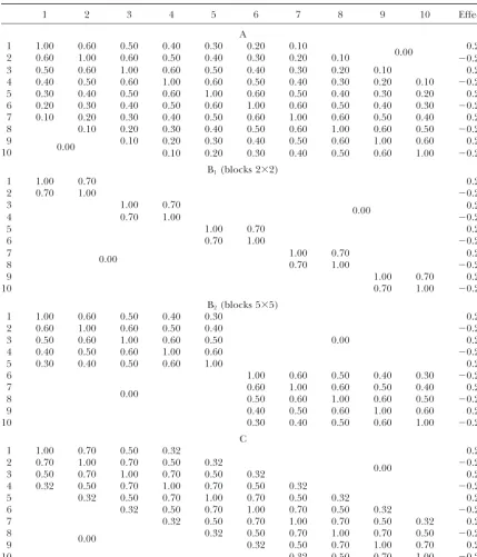
TABLE 1
Residual covariance matrices and QTL effects used in the simulations
1 2 3 4 5 6 7 8 9 10 Effect
A
1 1.00 0.60 0.50 0.40 0.30 0.20 0.10 0.25
2 0.60 1.00 0.60 0.50 0.40 0.30 0.20 0.10 0.00 ⫺0.25
3 0.50 0.60 1.00 0.60 0.50 0.40 0.30 0.20 0.10 0.25
4 0.40 0.50 0.60 1.00 0.60 0.50 0.40 0.30 0.20 0.10 ⫺0.25
5 0.30 0.40 0.50 0.60 1.00 0.60 0.50 0.40 0.30 0.20 0.25
6 0.20 0.30 0.40 0.50 0.60 1.00 0.60 0.50 0.40 0.30 ⫺0.25
7 0.10 0.20 0.30 0.40 0.50 0.60 1.00 0.60 0.50 0.40 0.25
8 0.10 0.20 0.30 0.40 0.50 0.60 1.00 0.60 0.50 ⫺0.25
9 0.10 0.20 0.30 0.40 0.50 0.60 1.00 0.60 0.25
10 0.00 0.10 0.20 0.30 0.40 0.50 0.60 1.00 ⫺0.25
B1(blocks 2⫻2)
1 1.00 0.70 0.25
2 0.70 1.00 ⫺0.25
3 1.00 0.70
0.00 0.25
4 0.70 1.00 ⫺0.25
5 1.00 0.70 0.25
6 0.70 1.00 ⫺0.25
0.00
7 1.00 0.70 0.25
8 0.70 1.00 ⫺0.25
9 1.00 0.70 0.25
10 0.70 1.00 ⫺0.25
B2(blocks 5⫻5)
1 1.00 0.60 0.50 0.40 0.30 0.25
2 0.60 1.00 0.60 0.50 0.40 ⫺0.25
3 0.50 0.60 1.00 0.60 0.50 0.00 0.25
4 0.40 0.50 0.60 1.00 0.60 ⫺0.25
5 0.30 0.40 0.50 0.60 1.00 0.25
6 1.00 0.60 0.50 0.40 0.30 ⫺0.25
7
0.00 0.60 1.00 0.60 0.50 0.40 0.25
8 0.50 0.60 1.00 0.60 0.50 ⫺0.25
9 0.40 0.50 0.60 1.00 0.60 0.25
10 0.30 0.40 0.50 0.60 1.00 ⫺0.25
C
1 1.00 0.70 0.50 0.32 0.25
2 0.70 1.00 0.70 0.50 0.32
0.00 ⫺0.25
3 0.50 0.70 1.00 0.70 0.50 0.32 0.25
4 0.32 0.50 0.70 1.00 0.70 0.50 0.32 ⫺0.25
5 0.32 0.50 0.70 1.00 0.70 0.50 0.32 0.25
6 0.32 0.50 0.70 1.00 0.70 0.50 0.32 ⫺0.25
7 0.32 0.50 0.70 1.00 0.70 0.50 0.32 0.25
8
0.00 0.32 0.50 0.70 1.00 0.70 0.50 ⫺0.25
9 0.32 0.50 0.70 1.00 0.70 0.25
10 0.32 0.50 0.70 1.00 ⫺0.25
The four multitrait sets (A, B1, B2, and C) were used in Monte Carlo experiments presented in Table 2 and Figures 2 and 3. The trait complex B1includes five pairs of traits with nonzero correlation (0.7) only within pairs; likewise, trait complex B2includes two five-trait blocks with nonzero correlations only within the blocks. Empty cells in the covariance matrices correspond to zero correlation coefficients.
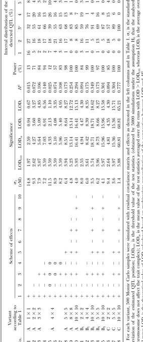
this trend reflects the fact that the increasingH2caused the LOD as a function of chromosomal position (l): at highH2values the function LOD(l) is more steep than by joint multiple-trait analysis results not only in higher
LOD values and detection power, but also in increased at small H2 (Figure 3). Clearly, increased precision of the estimated QTL position should also allow a more probability to find the QTL in the true interval (interval
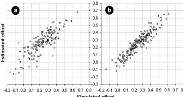
3; see footnote a in the right column of Table 2). At accurate estimation of the QTL effect. This is indeed the case, as illustrated by Figure 4. The increase inH2 the level of an individual experiment, the increased
tion 1 obtained byLanderandBotstein(1989) for a single trait, and generalized byKorolet al.(1995) for two-trait analysis, also holds in a general multivariate case. The last statement follows from the fact that herita-bility of a complex of noncorrelatedtraits with a single QTL affecting only one trait can be represented as
H2
D⫽1⁄4D2/(1⫹1⁄4D2), whereDis the multivariate effect and2the residual variance for the “integral” trait de-scribed inThe numerical procedures of interval analysis.
Example 2: Interval-specific estimation of the covariance
matrix:Another comment concerns the interval
speci-ficity that is a characteristic of our approach to defining the elements of the residual covariance matrix, RR. If, instead of that, one uses the total (interval-indepen-dent) covariance matrix defined on the entire sample, the efficiency of mapping may be lowered. The
numeri-Figure 2.—Multivariate heritability as a predictor of the cal example with a three-trait complex shown in Table
LOD value (affecting QTL detection power) and mapping
3 illustrates the difference between the two approaches. resolution. Right-hand scale, ELOD (䊊), left-hand scale, SL
One can easily see that if the approach based on total (standard deviation of the estimated QTL position;䊉). The
covariance matrix is employed, instead of our interval-graphs are based on Monte Carlo simulations described in
Table 1 and partially represented in Table 2. specific procedure, a reduction in the LOD value (hence lower detection power) and increase in the bias (␦) and standard variation () of the estimated QTL may justify a saturation of the chromosomal region in effects (di) and, especially, chromosomal position (L), the detected QTL by additional markers. This may allow may be obtained. Note that in the foregoing example a reduction of the chances of incorrect QTL location only a single QTL was simulated in the mapping popula-and finer QTL mapping, as well as an attempt at resolv- tion. The difference between the methods derives from ing the pleiotropy-linkage alternative (JiangandZeng the noncorrespondence between the residual correla-1995;Almasyet al.1997;Lebretonet al.1998;Korol tion matrix and the directions of the pleitropic effects.
et al.1998a;Roninet al.1999). Nevertheless, in some cases, where the total covariance
It is noteworthy that ELOD calculated on the basis matrix does not differ strongly fromRR, the loss will be ofH2
Tappeared to be a very good predictor of the aver- less pronounced (seeManginet al.1998).
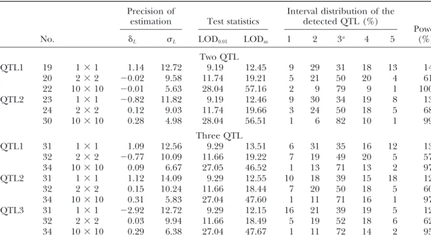
aged LOD obtained from Monte Carlo simulations (see Example 3: Multiple QTL: We now illustrate the effi-the column LODmin Table 2). This indicates that Equa- ciency of the proposed algorithm in situations with more than one QTL segregating in the mapping population. We simulated two and three identical unlinked QTL with the residual 10 ⫻ 10 covariance matrix equal to that of example 10 and the same pleiotropic effects (see Tables 1 and 2). As before, 500 Monte Carlo runs were made. The results (Table 4) confirm the previous con-clusion: a dramatic improvement can be achieved by use of joint analysis of the correlated traits. Note that segregation for one or two additional QTL resulted in an increase in the residual variances (as compared with Example 1). Consequently, we obtained a slightly lower detection power and a lower mapping precision. For the 10-trait analysis, the standard deviation of the estimated QTL position (SL) increased from 4.0 to 5.0–5.6 cM in case of two QTL and to 5.8–6.7 cM in the case of three QTL. Clearly, this reduction in mapping precision can be recovered by a composite interval mapping approach (Zeng 1994; Jansen and Stam 1994) but within the framework of multiple-trait analysis.
Significance of the detected effects:Testing for
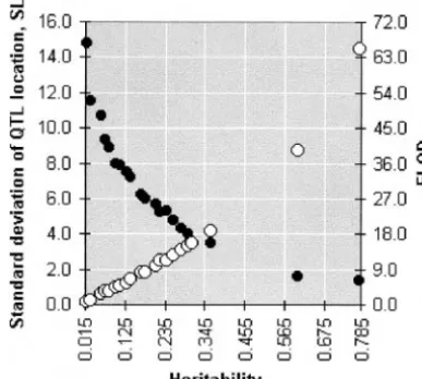
sig-Figure 3.—The dependence of the LOD function on the
nificance is a difficult problem in QTL mapping analysis, number of traits. The numbers in the solid circles indicate the
especially when multiple intervals and/or multiple traits number of traits; the simulated position of the QTL is marked
Figure 4.—Improved correspondence be-tween the simulated and estimated QTL effects in multiple-trait analysis as compared to single-trait analysis. (a) Single-single-trait analysis; (b) 10-single-trait analysis (based on the first example of Table 1).
Kruglyak1995;Welleret al.1998). To get the critical going aspects are illustrated in a simulated example with level of the test statistics in the foregoing analysis we seven quantitative traits and a chromosome with five employed Monte Carlo simulations with parameters cor- intervals (10 cM each) with a QTL residing in the middle responding to H0 (no QTL in the chromosome, with of the third interval. The pleiotropic effects of the simu-5000 runs per each variant). Clearly, this technique can lated QTL, the residual correlation matrix, and residual also be used for real data analysis, but it would be much variances were as shown in Table 5. The results can be more preferable to take into account the distribution outlined as follows:
properties of the real data set. The best way to do this
i. To evaluate the significance of the QTL detected in testing significance is the permutation test (Doerge
by using seven-dimensional mapping analysis, the and Churchill 1996). A few different, although
re-entire vector of trait values was reshuffled relative lated, questions about the significance of the results can
to the marker scores (while retaining the structure be recognized in the multiple-trait procedure: (i) What
within the trait complex). For each such permutated is the significance level of the detected QTL?, (ii) which
data set, the mapping procedure was applied, re-traits significantly contributed to the criterion
(multivar-sulting in a corresponding value of the test statistics iate LOD score)?, and (iii) which traits depend
signifi-LOD score. This process was repeated many times cantly on the detected QTL? The difference between
(10,000 in our experiment). The significance of the the second question and the third is caused by the fact
H0hypothesis (no effect of the considered chromo-that the information value of a trait may derive from its
some on the multivariate trait complex) is calculated correlation to other traits of the complex, from the
as the proportion of permutation runs that resulted pleiotropic effect of the QTL on this trait, or from both
in LOD values equal to or exceeding LOD* obtained these factors (see Figure 1).
Example 4: Selecting significant traits and effects:The fore- on the nonpermutated data.
TABLE 3
Comparison of the QTL mapping results obtained by the proposed method (based on interval-specific determination of the residual covariance matrixRR) and by using the total covariance matrix (Rtotal)
Effect
Matrix LOD Parameter L(cM) d1 d2 d3
RR 48.10 ␦ 0.02 0.010 ⫺0.003 0.007
1.44 0.048 0.050 0.050
Rtotal 27.58 ␦ 0.04 0.027 ⫺0.023 0.018
3.60 0.069 0.068 0.064
Trait 1 2 3 Effect
1 1.00 0.01 0.70 ⫹0.75
2 0.01 1.00 0.70 ⫺0.75
3 0.70 0.70 1.00 ⫹0.50
TABLE 4
The effect of the number of traits on efficiency of QTL mapping analysis with multiple QTL segregating in the mapping population
Precision of Interval distribution of the
estimation Test statistics detected QTL (%)
Power
No. ␦L L LOD0.01 LODm 1 2 3a 4 5 (%)
Two QTL
QTL1 19 1⫻1 1.14 12.72 9.19 12.45 9 29 31 18 13 14
20 2⫻2 ⫺0.02 9.58 11.74 19.21 5 21 50 20 4 61
22 10⫻10 ⫺0.01 5.63 28.04 57.16 2 9 79 9 1 100
QTL2 23 1⫻1 ⫺0.82 11.82 9.19 12.46 9 30 34 19 8 13
24 2⫻2 0.12 9.03 11.74 19.66 3 24 50 18 5 68
30 10⫻10 0.28 4.98 28.04 56.51 1 6 82 10 1 99
Three QTL
QTL1 31 1⫻1 1.09 12.56 9.29 13.51 6 31 35 16 12 13
32 2⫻2 ⫺0.77 10.09 11.66 19.22 7 19 49 20 5 57
34 10⫻10 0.09 6.67 27.05 46.52 1 13 71 13 2 97
QTL2 31 1⫻1 1.12 14.09 9.29 12.55 10 18 39 15 18 12
32 2⫻2 0.15 10.24 11.66 18.44 7 20 50 18 5 60
34 10⫻10 0.31 5.83 27.04 47.60 1 11 71 16 1 97
QTL3 31 1⫻1 ⫺2.92 12.72 9.29 12.15 16 21 39 19 5 12
32 2⫻2 0.03 9.94 11.66 18.49 5 19 52 18 6 62
34 10⫻10 0.29 6.38 27.04 47.67 1 11 72 14 2 95
The parameters␦LandL denote the bias and standard deviation of the estimated QTL position; LOD0.01 is the threshold value of the test statistics (obtained by 5000 simulations under the assumption H0 that the analyzed chromosome does not affect the trait complex); LODmis the mean value of the test statistics averaged over the runs with LOD⬎LOD0.01.
aThe simulated position of each of the two or three QTL on the corresponding chromosomes was the middle of the third interval.
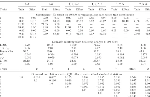
ii. The second test aimed to evaluate the significance traits. Namely, we calculate the proportion of per-of contributions per-of each per-of the traits for the QTL mutated cases where the estimated QTL effect for detection power. This test is conducted separately the considered trait xi fits the condition abs(di)ⱖ for each trait. For this, the individual values of the abs(d*i ), whered*i is the estimated effect on traitxi trait under consideration are reshuffled relative to obtained on initial (not reshuffled) data.
the remaining data (the other trait values and
In the example of Table 5, trait 7 displayed the lowest marker scores). The resulting data set is treated as
contribution and hence was removed after the first step. before and the proportion of runs with LOD ⱖ
Reevaluation of the remaining complex revealed the LOD* is used as the measure of significance of the
next candidate to remove, trait 3, and then, similarly, trait contribution. The permutations are always
per-trait 4. All the remaining per-traits (1, 2, 5, and 6) showed formed regarding all the traits included in the
significant contribution. This trait complex provides model independently of the contribution value of
also the narrowest confidence interval for the estimated the remaining traits. Clearly, some traits may prove
QTL position (L), as shown by the results of bootstrap to be insignificant because they contribute the same
analysis. The last result means that maintenance of ex-information as one (or a few) of the remaining traits.
cessive (noninformative) traits is not neutral, a reduced Thus, one can exclude insignificant traits from
con-precision of the estimated QTL position being the pen-sideration by creating a new trait set that does not
alty. Filtering out of the nonsignificant traits should include the insignificant traits(s). This procedure
affect the QTL detection power, but further reduction should be applied by simple steps, excluding only
of the trait complex by removing the significant traits one trait per step and repeating the permutation
may result in a reduced power and lowered mapping test for the remainder. The last warning is important
precision (see the characteristics obtained for the last because after excluding one of the traits at some
two trait combinations, 1, 2, 5, and, especially, 2, 5, 6). step, the significance of contributions of the
re-An example of application to real data:We illustrate maining traits may change.
the efficiency of the proposed approach using real data iii. The same procedure as in (ii) can be used to test
TABLE 5
Permutation test of significance for the contribution of the traits: the multitrait LOD and the pleiotropic effects of the QTL
1–7 1–6 1, 2, 4–6 1, 2, 5, 6 1, 2, 5 2, 5, 6
Traits Trait Effect Trait Effect Trait Effect Trait Effect Trait Effect Trait Effect
Significance (%) based on 10,000 permutations for each tested trait combination
1 0.00 0.07 0.00 0.07 0.00 0.08 0.00 0.07 0.00 0.08 — —
2 0.03 84.16 0.02 84.23 0.02 83.87 0.02 83.01 1.18 85.10 71.99 83.14
3 21.76 5.10 21.85 5.08 — — — — — — — —
4 18.46 1.56 19.28 1.56 11.94 1.59 — — — — — —
5 0.00 0.00 0.00 0.00 0.00 0.00 0.00 0.00 0.01 0.00 0.01 0.00
6 0.20 63.17 0.19 63.15 0.16 62.56 0.15 61.52 — — 73.06 62.62
7 58.40 41.10 — — — — — — — — — —
Estimates resulting from bootstrap analysis (1000 runs)
LODm 12.72 12.43 11.90 11.16 8.83 4.88
LODm 2.86 2.87 2.71 2.71 2.48 1.86
Power (%) 99.5 99.6 99.7 99.7 95.9 47.4
H2 0.346 0.324 0.304 0.290 0.204 0.172
H2 0.086 0.079 0.078 0.070 0.062 0.083
L(cM) 24.12 24.17 24.53 23.81 23.58 21.03
L 5.26 5.09 5.00 3.88 5.22 7.04
Traits 1 2 3 4 5 6 7 Effect
Occurred correlation matrix, QTL effects, and residual standard deviations
1 1.0 0.618 0.062 0.165 0.054 0.155 0.156 0.504 0.955
2 1.0 0.126 0.020 0.112 0.723 0.156 0.037 1.013
3 1.0 0.236 0.072 0.092 0.007 0.281 1.002
4 1.0 ⫺0.069 ⫺0.112 0.032 0.283 1.088
5 1.0 0.034 ⫺0.050 0.674 0.982
6 1.0 0.105 0.044 0.968
7 1.0 ⫺0.149 0.960
The simulated effects, residual correlation matrix, and standard deviations are as shown in the bottom; note that one out of seven traits, no. 7, was simulated as “noise”, trait 2 was independent on the QTL but correlated with traits 1 and 6.
On the basis of the permutation test, the significance of contribution to the LOD score as well as the QTL effect was evaluated for each trait. After the first step, trait 7 that appeared to have the lowest contribution was removed. Reevaluation of the remainder complex revealed the next candidate to remove, trait 3, and then, similarily, trait 4. All the remainder traits, 1, 2, 5, and 6, show significant contribution. This complex (italic) also provides the narrowest confidence interval for the estimated QTL position (L), as shown by the results of bootstrap analysis. This filtering out of the nonsignificant traits did not affect the QTL detection power, whereas further reduction of the trait complex by removing the significant traits may result in a reduced power and lowered mapping precision (see the characteristics obtained for the last two trait combinations).
morphological quantitative traits. The experiment was field trials conducted in Neve Yaar Agricultural Experi-mental Station, Israel, during the 1997–1998 cropping performed on an F2/F3 mapping population derived
from a cross between a highly stripe-rust-resistant wild season. Eleven quantitative traits were scored on F3 prog-eny (forⵑ10 individual plants from each family): plant emmer wheat Triticum dicoccoides (accession no. H52,
from Mt. Hermon, Israel) and aT. durumcultivar, Lang- height (HT), plant heading date—the days from sowing to heading (HD); spike number/plant (SNP); spike don, released in North Dakota. The tetraploid wild
em-mer,T. dicoccoides, is the progenitor of cultivated wheat; weight/plant (SWP) including the grains, hulls, and
rachis; single spike weight (SSW); kernel number/plant hence, the genetic dissection of quantitative trait
differ-ences between the wild species and the cultivated crop (KNP); kernel number/spike (KNS); kernel number/ spikelet (KNL); 100-grain weight (GWH); grain yield/ is of great interest from the viewpoint of domestication
evolution. It is also important for the ever-increasing plant (YLD); and spikelet number/spike (SLS). A detailed QTL description of the obtained QTL map-utilization ofT. dicoccoidesas a rich genetic resource for
wheat improvement. The molecular markers [microsa- ping results on these traits will be presented elsewhere (J. H. Peng, A. B. Korol, T. Fahima, Y. I. Roninand tellites and amplified fragment length polymorphisms
(AFLP)] were scored on 150 F2individuals resulting in E. Nevo, unpublished results). Here we employ the obtained data only to illustrate the efficiency of the a rather dense genetic map (Peng et al. 2000). The
chro-TABLE 6
Interval analysis of a multitrait complex that includes 11 morphological traits scored in F2/F3mapping population of wheatTriticum durum⫻T. dicoccoides(Penget al.2000)
QTL detection power (%) at three significance levels
No. of LODf Significance, by
traits LODf LL(cM) ␣ ⫽0.05 ␣ ⫽0.01 ␣ ⫽0.001 permutation test
1 4.38 271 91 71 42 0.011
1.63 74
11 19.71 265 100 100 100 ⬍0.0001
3.43 36
5 13.82 262 100 100 99 ⬍0.0001
2.91 30
The example is based on markers of chromosome 7A.
The results of single-trait interval analysis (for trait GWH) are compared with those of the entire 11-trait complex and the “filtered” five-trait complex obtained by excluding nonsignificant traits (as in the example shown in Table 5). The traits remaining in the five-trait complex are: GWH, YLD, HD, HT, and SWP. The significance level for each trait and trait complex was calculated using a permutation test (10,000 runs). In addition to the analysis of the initial data set, 1000 bootstrap runs were conducted, enabling us to evaluate the QTL detection power and precision of the parameter estimates. LODfandLODfare the mean value and standard deviation of the test statistics estimated on the basis of 1000 bootstrap runs; correspondingly,Land Lare the QTL map position and its standard deviation.
mosome 7A. With single-trait analysis applied separately to each of the traits, only one significant QTL was found on 7A, for trait GWH, with significance level ⵑ0.01 (Table 6). This level should be corrected for multiple comparisons, taking into account the fact that the ana-lyzed traits are correlated (e.g., by using the method based on factor analysis, as suggested bySpelmanet al.
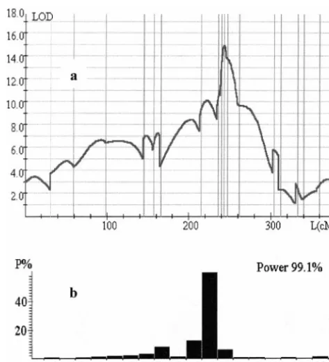
1996). Therefore, the corrected significance will be even worse. The mapping precision evaluated by bootstrap analysis is not high (L⫽74 cM), as one would expect for the modest population size employed (n ⫽ 150). Therefore, it makes sense to attempt improvement of the mapping by utilizing the information contained in the entire trait complex, owing to possible pleiotropic effects of the putative QTL and/or correlations between GWH and the remaining traits. This was done exactly in the same way as described in the foregoing simulated example presented in Table 5. First, the entire complex of 11 traits was analyzed and then the traits that did not contribute significantly to the test statistics were removed. The results presented in Table 6 and Figure 5 show a more than twofold increase in the mapping precision (Ldecreased from 74 to 30 cM) and an in-crease in detection power that is especially clear at
higher significance level (98.9% vs.42.9%). Figure5.—Joint analysis of 11 traits scored in F2/F3 map-ping population of wheatTriticum durum⫻T. dicoccoidesusing markers of chromosome 7A. The results of removing nonsig-DISCUSSION nificant traits are presented. (a) LOD score distribution along chromosome 7A for the 5-trait complex (GWH, YLD, HD, A multivariate generalization of our previous two-trait
HT, and SWP). (b) Interval distribution of the maximum LOD QTL mapping analysis (Korolet al.1987, 1995, 1998a; values along chromosome 7A based on 1000 bootstrap runs. Roninet al.1995, 1999; see alsoJiangandZeng1995) Both graphs are outputs of the MultiQTL package (http://
to other situations (e.g., analyzing F3 populations), to into account all available information concerning the deal with linked QTL (similar to the analysis ofKorolet patient. However, this does not mean that increasing
al.1998a;Roninet al.1999), to combine it with selective the number of traits to be analyzed simultaneously will genotyping design (Ronin et al. 1998;Henshall and necessarily improve the quality of the QTL mapping Goddard1999), or to adopt composite interval map- results. A technical obstacle with high dimensionality is ping (Jansenand Stam 1994; Zeng1994). Especially an increasing probability that many loci may affect the promising may be its application to fine mapping (Y. I. analysis along the chromosome, whereas a small-to-mod-Ronin, E. Britvin, E. NevoandA. B. Korol, unpub- erate population size could hardly justify fitting more lished results). Indeed, the dramatic increase in map- than two or three linked QTL simultaneously. Another ping resolution derived from using the entire multivari- problem is the interpretation of the results. Therefore, ate complex, as compared with univariate or even in choosing the initial set of traits for joint QTL analysis, bivariate analysis, effectively increases the scoreD2
nthat one may find it reasonable to restrict such sets by function-was found to affect the mapping resolution (Darvasi ally related traits. The examples presented in this article, andSoller1997). Consequently, it becomes reasonable on both simulated and real data, show that maintenance to saturate the revealed intervals by additional markers of excessive traits in the model may be penalized. These even at modest population sizes like 200–500 individu- concerns indicate that in spite of high potential and bio-als; usually this is pointless because with small effects logical “compatibility” of the multiple-trait analysis to the no increase in precision is expected by addition of new main targets of QTL analysis, a lot of work remains to be markers to the map (Darvasiet al. 1993). Therefore, done to fully extract the mapping information hidden in the transition from a single- or even two-trait analysis the collected data.
to treatment of genuine multiple-trait complexes sig- An additional complication that is worth mentioning nificantly improves all aspects of utilizing the mapping is the possible effect of the model assumption on the information contained in the data. obtained results. It was shown earlier that for testing However, the application of multivariate complexes for linkage, erroneous models may lead to valid tests not only increases the QTL detection power, mapping for linkage (Wright and Kong 1997). For example, resolution, and estimation accuracy but it may also in- QTL mapping analysis may be quite robust to violations crease the power of discriminating various important of the assumption of normality in single-trait situations hypotheses that concern the genetic architecture of (Korolet al.1996b) and more sensitive in multivariate complex traits, such as linkagevs. pleiotropy (Schork ones. Likewise, the assumption of homoscedastic
distri-et al. 1994;Jiang andZeng1995; Almasy et al. 1997; butions (i.e., equal residual variances in QTL groups)
Lebretonet al.1998;Roninet al.1999), genetic interac- that is usually applied automatically may be wrong, lead-tion within and across QTL (additivevs. dominant or ing to reduced QTL detection power and biased esti-overdominant effects, and additivevs. epistatic effects mates of parameters. On the contrary, if a correct model or canalization;Roninet al.1999;ShookandJohnson is fitted, this may increase the detection power and 1999), and QTL-environment interaction (Fry et al. mapping accuracy compared to situations when no such
1998; Korol et al. 1998b). Multivariate QTL analysis disturbances exist. We demonstrated these effects ear-may be helpful in genetic dissection of such types of lier for single- and two-trait analysis (
Korolet al.1995, complex traits as multifactorial diseases (Mansfieldet
1996a). Especially important is the assumption of a
sin-al.1997), development (Wuet al.1999), longevity and
gle QTL per chromosome, which being violated may aging (Nuzhdin et al. 1997), behavior (Plomin and
lead to the LOD score peaking in the wrong place (see Craig 1997; Wehner et al. 1997), fitness-related trait
KnottandHaley1992;WrightandKong1997). For complexes and species differentiation (Zeng et al.
the two-trait case we found that joint analysis of corre-2000), heterosis (Xiao et al. 1995), marker-assisted
lated traits increases the power of the test aimed to breeding (LandeandThompson1990;Visscheret al.
discriminate between the single QTL and two-linked 1996), characterizing the regulatory networks of
struc-QTL situations (Ronin et al. 1999). All these aspects tural genes (Damervalet al. 1994), bridging between
should be taken into account in multivariate QTL anal-gene-structure-and-function studies (e.g., when looking
ysis. for functions of massively expressed sequence tags;
Lah-The described approach is implemented in the bib-Mansaiset al.1999), analyzing the genetic
transmis-MultiQTL package (http://www.transmis-MultiQTL.com) for sion system (breeding system, recombination, and
muta-both single- and two-linked QTL models. tion control; Korol et al. 1994; Bernacchi and
We thank M. Soller, J. Weller, G. Churchill, and three anonymous
Tanksley1997), and so on.
referees for helpful comments and suggestions on the first version
As a not-so-remote analogy, one could compare the
of the manuscript. This study was supported by the Israeli Science
situation of multivariate QTL analysis with that
charac-foundation (grants 02198 and 9048/99), the United States-Israel
Bina-teristic of medical diagnoses: excluding simple situa- tional Science Foundation (grant 4556), and the German-Israeli Coop-tions, a good physician will never rely on one trait (symp- eration Project (DIP project funded by the Internationales Bu¨ ro
Deutsch-Israelische des BMBF Projektkooperation).
1999 A successful strategy for comparative mapping with human
LITERATURE CITED
ESTs: 65 new regional assignments in the pig. Mamm. Genome
10:145–153.
Allison, D. B., B. Thiel, P. St. Jean, R. C. Elston, M. C. Infante
et al., 1998 Multiple phenotype modeling in gene-mapping stud- Lande, R.,andR. Thompson,1990 Efficiency of marker assisted
selection in the improvement of quantitative traits. Genetics124:
ies of quantitative traits: power advantages. Am. J. Hum. Genet.
63:1190–1201. 743–756.
Lander, E. S.,andD. Botstein,1989 Mapping Mendelian factors
Almasy, L., T. D. DyerandJ. Blangero,1997 Bivariate quantitative
trait linkage analysis: pleiotropy versus co-incident linkages. underlying quantitative traits using RFLP linkage maps. Genetics
121:185–199. Genet. Epidemiol.14:953–958.
Amos, C. I., R. C. Elston, G. E. Bonney, B. J. Keats andG. S. Lander, E.,andL. Kruglyak,1995 Genetic dissection of complex traits: guidelines for interpreting and reporting linkage results.
Berenson,1990 A multivariate method for detecting genetic
linkage, with application to a pedigree with an adverse lipoprotein Nat. Genet.11:241–247.
Lebowitz, B. J., M. SollerandJ. S. Beckmann,1987 Trait-based phenotype. Am. J. Hum. Genet.47:247–254.
Bernacchi, D.,andS. D. Tanksley,1997 An interspecific backcross analyses for the detection of linkage between marker loci and quantitative trait loci in crosses between inbred lines. Theor. ofLycopersicon esculentum⫻L. hirsutum: linkage analysis and a QTL
study of sexual compatibility factors and floral traits. Genetics147: Appl. Genet.73:556–562.
Lebreton, C. M., P. M. Visscher, C. S. Haley, A. Semikhodskiiand 861–877.
Boomsma, D. I.,andC. V. Dolan,1998 A comparison of power to S. A. Quarrie, 1998 A nonparametric bootstrap method for testing close linkage vs. pleiotropy of coincident quantitative trait detect a QTL in sib-pair data using multivariate phenotypes, mean
phenotypes, and factor scores. Behav. Genet.28:329–340. loci. Genetics150:931–943.
Mangin, B., P. ThoquetandN. Grimsley, 1998 Pleiotropic QTL
Damerval, C., A. Maurice, J. M. Josse and D. de Vienne,
1994 Quantitative trait loci underlying gene product variation: a analysis. Biometrics54:88–99.
Mansfield, T. A., D. B. Simon, Z. Farfel, M. Bia, J. R. Tucciet al., novel perspective for analyzing regulation of genome expression.
Genetics137:289–301. 1997 Multilocus linkage of familial hyperkalaemia and hyper-tension, pseudohypoaldosteronism type II, to chromosomes
Darvasi, A.,andM. Soller,1994 Selective DNA pooling for
deter-mination of linkage between a molecular marker and a quantita- 1q31-42 and 17p11-q21. Nat. Genet.16:202–205.
Motro, U.,andM. Soller,1993 Sequential sampling in determin-tive trait locus. Genetics138:1365–1373.
Darvasi, A.,andM. Soller, 1997 A simple method to calculate ing linkage between marker loci and quantitative trait loci. Theor. Appl. Genet.85:658–664.
resolving power and confidence interval of QTL map position.
Behav. Genet.27:125–132. Nuzhdin, S. V., E. G. Pasyukova, C. L. Dilda, Z-B. ZengandT. F. Mackay,1997 Sex-specific quantitative trait loci affecting
lon-Darvasi, A., A. Weinreb, V. Minke, J. I. WellerandM. Soller,
1993 Detection marker-QTL linkage and estimating QTL gene gevity inDrosophila melanogaster.Proc. Natl. Acad. Sci. USA94:
9734–9739. effect and map location using a saturated genetic map. Genetics
134:943–951. Olson, J. M., S. Rao, K. JacobsandR. C. Elston,1999 Linkage of chromosome 1 markers to alcoholism-related phenotypes by
Doerge, R. W.,andG. A. Churchill,1996 Permutation tests for
multiple loci affecting a quantitative character. Genetics142: sib pair linkage analysis of principal components. Genet. Epide-miol.17(Suppl. 1): S271–276.
285–294.
Fry, J. D., S. V. Nuzhdin, E. G. PasyukovaandT. F. Mackay,1998 Peng, J. H., A. B. Korol, T. Fahima, M. S. Ro¨ der, Y. I. Roninet al., 2000 Molecular genetic maps in wild emmer wheat,Triticum
QTL mapping of genotype-environment interaction for fitness
inDrosophila melanogaster.Genet. Res.71:133–141. dioccoides: genome-wide coverage, massive negative interference,
and putative quasi-linkage. Genome Res.10:1509–1531.
Henshall, J. M.,andM. E. Goddard,1999 Multiple-trait mapping
of quantitative trait loci after selective genotyping using logistic Plomin, R., and I. Craig, 1997 Human behavioural genetics of cognitive abilities and disabilities. Bioessays19:1117–1124. regression. Genetics151:885–894.
Jansen, R. C.,andP. Stam, 1994 High resolution of quantitative Ronin, Y. I., V. M. KirzhnerandA. B. Korol,1995 Linkage between loci of quantitative traits and marker loci. Multitrait analysis with traits into multiple loci via interval mapping. Genetics136:1447–
1455. a single marker. Theor. Appl. Genet.90:776–786.
Ronin, Y. I., A. B. KorolandY. Weller,1998 Selective genotyping
Jiang, C., andZ-B. Zeng, 1995 Multiple trait analysis of genetic
mapping for quantitative trait loci. Genetics140:1111–1127. to detect quantitative trait affecting multiple traits. Theor. Appl. Genet.97:1169–1178.
Knott, S. A.,andC. S. Haley,1992 Aspects of maximum likelihood
methods for mapping of quantitative trait loci in line crosses. Ronin, Y. I., A. B. KorolandE. Nevo,1999 Single- and multiple-trait analysis of linked QTL: some asymptotic analytical approxi-Genet. Res.60:139–151.
Korol, A. B., I. A. PreygelandN. Bocharnikova,1987 Linkage mation. Genetics151:387–396.
Schmalhausen, I. I.,1942 Organism as a Whole Entity in the Individual
between loci of quantitative traits and marker loci. 5.
Simultane-ous analysis of a set of markers and quantitative traits. Genetika and Historic Development.USSR Academy of Sciences, Moscow-Leningrad (in Russian).
23:1421–1431 (English translation in Sov. Genet. 1988,23:996–
1004). Schork, N. J., A. B. Weder, M. TrevisanandM. Laurenzi,1994 The contribution of pleiotropy to blood pressure and body-mass
Korol, A. B., I. A. PreygelandS. I. Preygel,1994 Recombination
Variability and Evolution.Chapman & Hall, London. index variation: the Gubbio Study. Am. J. Hum. Genet.54:361–
373.
Korol, A. B., Y. I. RoninandV. M. Kirzhner,1995 Interval mapping
of quantitative trait loci employing correlated trait complexes. Shook, D. R.,andT. E. Johnson,1999 Quantitative trait loci affect-ing survival and fertility-related traits inCaenorhabditis elegansshow Genetics140:1137–1147.
Korol, A. B., Y. I. Ronin, Y. Tadmor, A. Bar-Zur, V. M. Kirzhner genotype-environment interactions, pleiotropy and epistasis. Ge-netics153:1233–1243.
et al., 1996a Estimating variance effect of QTL: an important
prospect to increase the resolution power of interval mapping. Soller, M.,andJ. S. Beckmann,1990 Marker-based mapping of quantitative trait loci using replicated progeny. Theor. Appl. Genet. Res.67:187–194.
Korol, A. B., Y. I. Ronin and V. M. Kirzhner, 1996b Linkage Genet.80:205–208.
Spelman, R. J., W. Coppieters, L. Karim, J. A. van Arendonkand between loci of quantitative traits and marker loci. Resolution
power of three statistical approaches in single marker analysis. H. Bovenhuis,1996 Quantitative trait loci analysis for five milk production traits on chromosome six in the Dutch Holstein-Biometrics52:426–441.
Korol, A. B., Y. I. Ronin, P. HayesandE. Nevo,1998a Multi-interval Friesian population. Genetics144:1799–1808.
Visscher, P. M., C. S. Haley and R. Thompson, 1996 Marker-mapping of correlated trait complexes: simulation analysis and
evidence from barley. Heredity80:273–284. assisted introgression in backcross breeding programs. Genetics
144:1923–1932.
Korol, A. B., Y. I. RoninandE. Nevo,1998b Approximated analysis
of QTL-environmental interaction with no limits on the number Wehner, J. M., R. A. Radcliffe, S. T. Rosmann, S. C. Christensen, D. L. Rasmussenet al., 1997 Quantitative trait locus analysis of of environments. Genetics148:2015–2028.
Weller, J. I., G. R. Wiggans, P. M. Van RadenandM. Ron,1996 Wu, W. R., W. M. Li, D. Z. Tang, H. R. LuandA. J. Worland,1999 Application of a canonical transformation to detection of quanti- Time-related mapping of quantitative trait loci underlying tiller tative trait loci with the aid of genetic markers in a multi-trait number in rice. Genetics151:297–303.
experiment. Theor. Appl. Genet.92:998–1002. Xiao, J., J. Li, L. YuanandS. D. Tanksley,1995 Dominance is the
Weller, J. I., J. Z. Song, D. W. Heyen, H. A. LewinandM. Ron, major genetic basis of heterosis in rice as revealed by QTL analysis 1998 A new approach to the problem of multiple comparisons using molecular markers. Genetics140:745–754.
in the genetic dissection of complex traits. Genetics150:1699– Zeng, Z-B.,1994 Precise mapping of quantitative trait loci. Genetics
1706. 136:1457–1468.
Williams, J. T., P. Van Eerdewegh, L. AlmasyandJ. Blangero, Zeng, Z-B., J. Liu, L. F. Stam, C. H. Kao, J. M. Merceret al., 2000
1999 Joint multipoint linkage analysis of multivariate qualitative Genetic architecture of a morphological shape difference be-and quantitative traits. I. Likelihood formulation be-and simulation tween twoDrosophilaspecies. Genetics154:299–310.
results. Am. J. Hum. Genet.65:1134–1147.
Wright, F. A.,andA. Kong,1997 Linkage mapping in experimental Communicating editor:G. A. Churchill