Design of Discrete Hartley Transform using
Parallel and Partition Multiplier Method
Shikha Pandey1, Hema Singh2
M. Tech. Scholar, Department of Electronics and Communication, TIT, Bhopal, India1 Professor, Department of Electronics and Communication, TIT, Bhopal, India2
ABSTRACT: A Discrete Hartley Transform (DHT) is a real valued transform related to Discrete Fourier Transform (DFT) and Fast Fourier Transform (FFT) of a real valued sequence. In this paper radix-2 DHT algorithm using parallel multiplier and partition multiplier method are present. Discrete Hartley Transform (DHT) is basically used while converting real valued data from time domain into frequency domain. In order to calculate DHT which is of length 2N, where N is assigned as 3 and 4, a new algorithm is proposed for calculating the same. We have implemented parallel & partition multiplier along with Kogge Stone adder which is an improvement over simple multiplication that was achieved in conventional DHT. This paper shows an examination of conventional DHT calculation with proposed DHT calculation concerning mainly on delay and slice.
KEYWORDS: Parallel Multiplier, Partition Multiplier, Discrete Hartley Transform (DHT), Xilinx Software
I. INTRODUCTION
The data of various domains is processed as per their applications and is performed mainly by DSP (Digital Signal Processing). This includes applications in scientific, space, medical, industrial and commercial fields [1]. Each one of them needs processing huge data to collect useful information. A technique called transform is used in DSP to convert data in another form. In DSP, a family of transform for processing of data is available. The oldest technique, called Fourier analysis which is named after Jean baptiste joseph Fourier (1768-1830) who was a French mathematician and physicist. It was used mainly in case of periodic and continuous signals [2, 3]. Fourier series is basically a technique that decomposes the signal from time domain to a no. of sine and cosine waves in frequency domain is but it is not applicable in case of non-periodic signals. Fourier transforms that removes the drawbacks of Fourier series then came into existence and that is used in case of periodic and continuous signals. Fourier transform is not suitable for non-stationary signals. As both the transforms mentioned above are not applicable in case of discrete signals, hence Discrete time Fourier transform (DTFT) is designed for the signals that are not periodic and extend from positive to negative infinity and. Discrete Fourier transform came into existence as DTFT is not used in case of periodic discrete signals [4]. DFT is a numerically equivalent as that of FT that uses summation in place of integrals. It is used in case of all signals that repeat itself in a periodically which extend from positive to negative infinity. FFT is an improvement over DFT in case those involve complex parts. In such case computation becomes faster.
II. DISCRETE HARTLEY TRANSFORM
In 1942, R. V. L. Hartley proposed Discrete Hartley Transform. It is almost similar to Fast Fourier transform. The main difference between FFT and DFT is that DFT deals only with real inputs to real outputs without any complex value. DFT and DHT can be computed by each other. [5].
In other words, Discrete Hartley transform converts real values in time domain into real values in frequency domain, which involves decomposing of data in various stages using butterfly. The butterfly diagram is almost similar to that of FFT. The butterfly diagram of DHT is different in terms of coefficients. The coefficients are also increased simultaneously in number, with the increase as the number of DHT sequence length increases.
Let
N
4
be a power of two. For any real input sequence}
1
...
,...
2
,
1
,
0
:
)
(
{
x
i
i
N
X
(
k
)
DHT
(
N
){
x
((
i
)}
1 01
...
1
,
0
]
/
2
[
).
(
N iN
k
for
N
ki
cas
i
x
Where
cas
(
x
)
cos(
x
)
sin(
x
)
ALGORITHM FOR 16 POINT DHT-
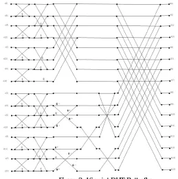
An algorithm to implement Discrete Hartley Transform that is comparatively fast is presented. The butterfly diagram for 16 point DHT design requires six stages. These consist of summing and various coefficient multiplying stages. Before initiating first stage, the data sequence will have to be arranged as in bit reversed pattern using a method like say permutation. Then, the first stage includes pairs of bit reversed patterns which are added and form eight terms. One third of the terms are again added and subtracted to form further three terms in the second stage [5, 6].
Any multiplication is excluded in first two stages. Rest of the terms is multiplied with the first coefficient. For the next stage again two new coefficients are introduced that is multiplied with the lower half of the third stage. Multiplying of coefficients stage precedes its summing stage in each stage. It is preceded, after coefficient multiplication by its summing stage that forms the common terms which is used in the final stage. Last stage sums up all the terms only. Finally a transformed data sequence which is ordered is obtained and does not require any permutation [7, 8].
Mathematical calculation for N=16
))
15
(
)
7
(
(
))
11
(
)
3
(
(
))
13
(
)
5
(
(
))
9
(
)
1
(
(
))
14
(
)
6
(
(
))
10
(
)
2
(
(
))
12
(
)
4
(
(
))
8
(
)
0
(
(
)
0
(
x
x
x
x
x
x
x
x
x
x
x
x
x
x
x
x
X
))}
15
(
)
7
(
(
))
11
(
)
3
(
{(
))}
15
(
)
7
(
(
))
11
(
)
3
(
{(
))
13
(
)
5
(
(
))
10
(
)
2
(
(
))
12
(
)
4
(
(
))
8
(
)
0
(
(
)
1
(
2 3 1x
x
x
x
c
x
x
x
x
c
x
x
x
x
c
x
x
x
x
X
DHTReal Inputs Real Outputs
))
15
(
)
7
(
(
))
11
(
)
3
(
(
))
10
(
)
2
(
(
))}
13
(
)
5
(
(
))
9
(
)
1
(
{(
)}
14
(
)
6
(
(
))
12
(
)
4
(
{(
))
8
(
)
0
(
(
)
2
(
1x
x
x
x
x
x
x
x
x
x
c
x
x
x
x
x
x
X
))}
15
(
)
7
(
(
))
11
(
)
3
(
{(
))}
15
(
)
7
(
(
))
11
(
)
3
(
{(
))
13
(
)
5
(
(
))
14
(
)
6
(
(
))
12
(
)
4
(
(
))
8
(
)
0
(
(
)
3
(
2 3 1x
x
x
x
c
x
x
x
x
c
x
x
x
x
c
x
x
x
x
X
))}
15
(
)
7
(
(
))
11
(
)
3
(
{(
))
13
(
)
5
(
(
))
9
(
)
1
(
(
))
14
(
)
6
(
(
))
10
(
)
2
(
(
))
12
(
)
4
(
(
))
8
(
)
0
(
(
)
4
(
x
x
x
x
x
x
x
x
x
x
x
x
x
x
x
x
X
))}
9
(
)
1
(
(
))
13
(
)
5
(
{(
))}
15
(
)
7
(
(
))
11
(
)
3
(
{(
))
13
(
)
5
(
(
))
10
(
)
2
(
(
))
12
(
)
4
(
(
))
8
(
)
0
(
(
)
5
(
2 3 1x
x
x
x
c
x
x
x
x
c
x
x
x
x
c
x
x
x
x
X
))}
15
(
)
7
(
(
))
11
(
)
3
(
{(
))}
12
(
)
4
(
(
))
10
(
)
2
(
{(
))
14
(
)
6
(
(
))
8
(
)
0
(
(
)
6
(
x
x
x
x
x
x
x
x
c
1x
x
x
x
X
))}
9
(
)
1
(
(
))
13
(
)
5
(
{(
))}
9
(
)
1
(
(
))
13
(
)
5
(
{(
))
14
(
)
6
(
(
))
12
(
)
4
(
(
))
8
(
)
0
(
(
)
7
(
1 3 2x
x
x
x
c
x
x
x
x
c
x
x
c
x
x
x
x
X
))
15
(
)
7
(
(
))
11
(
)
3
(
(
))
13
(
)
5
(
(
))
9
(
)
1
(
(
))
14
(
)
6
(
(
))
10
(
)
2
(
(
))
12
(
)
4
(
(
))
8
(
)
0
(
(
)
8
(
x
x
x
x
x
x
x
x
x
x
x
x
x
x
x
x
X
))}
15
(
)
7
(
(
))
11
(
)
3
(
{(
))}
15
(
)
7
(
(
))
11
(
)
3
(
{(
))
13
(
)
5
(
(
))
10
(
)
2
(
(
))
12
(
)
4
(
(
))
8
(
)
0
(
(
)
9
(
2 3 1x
x
x
x
c
x
x
x
x
c
x
x
x
x
c
x
x
x
x
X
))}
13
(
)
5
(
(
))
9
(
)
1
(
{(
)}
14
(
)
6
(
(
))
12
(
)
4
(
{(
))
8
(
)
0
(
(
)
10
(
x
x
x
x
x
x
c
1x
x
x
x
X
))}
15
(
)
7
(
(
))
11
(
)
3
(
{(
))}
15
(
)
7
(
(
))
11
(
)
3
(
{(
))
14
(
)
6
(
(
))
12
(
)
4
(
(
))
8
(
)
0
(
(
)
11
(
1 3 2x
x
x
x
c
x
x
x
x
c
x
x
c
x
x
x
x
X
))
15
(
)
7
(
(
))
11
(
)
3
(
(
))}
13
(
)
5
(
(
))
9
(
)
1
(
{(
))
14
(
)
6
(
(
))
10
(
)
2
(
(
))
12
(
)
4
(
(
))
8
(
)
0
(
(
)
12
(
x
x
x
x
x
x
x
x
x
x
x
x
x
x
x
x
X
))}
13
(
)
5
(
(
))
9
(
)
1
(
{(
))}
15
(
)
7
(
(
))
11
(
)
3
(
{(
))
10
(
)
2
(
(
))
12
(
)
4
(
(
))
8
(
)
0
(
(
)
13
(
1 3 2x
x
x
x
c
x
x
x
x
c
x
x
c
x
x
x
x
X
))
15
(
)
7
(
(
))
11
(
)
3
(
(
))
10
(
)
2
(
(
))
12
(
)
4
(
(
))
8
(
)
0
(
(
)
14
(
x
x
x
x
x
x
c
1x
x
x
x
X
))}
13
(
)
5
(
(
))
9
(
)
1
(
{(
))}
9
(
)
1
(
(
))
5
(
)
13
(
{(
))
14
(
)
6
(
(
))
12
(
)
4
(
(
))
8
(
)
0
(
(
)
15
(
1 3 2x
x
x
x
c
x
x
x
x
c
x
x
c
x
x
x
x
X
III. DIFFERENT TYPES OF MULTIPLIER
Parallel Multiplier: - Parallel multiplier and Kogge-Stone can compare with conventional method which is computed by parallel multiplier, full adder and half adder. Proposed technique provides less path delay and less area. Input sequence of Conventional method is much more than to proposed method, however proposed method has less propagation delay.
Figure 3: Block Diagram of Urdhwa Parallel Multiplier
recipient for high effective computerized gadgets according to concerning engendering delay. In the long run, all the outlining levels of advanced framework or IC's Packages rely upon number of doors in a solitary chip that is additionally rung base approach. Altered KS adder can be decreased with respect to the zone or number of entryways. If the first XOR gate removes from modified KS adder nothing will be changed for result but area and propagation delay will be reduced.
Figure 4: Block Diagram of Previous and Proposed Adder Partition Multiplier:-
In our proposed method the high speed Vedic multiplier method is replaced by the partition multiplier method which claims to provide a better speed and less propagation delay. Here we have used four multipliers M0, M1, N0 and N1 of
4-bit to perform 8-bit multiplication. The method used is the addition of all partial product formed by the cross multiplication of one bit with another. The LSB bits of first multiplier M0 (3-0) add with LSB bits N0 (3-0) of the final
output t1. Padding n/2-bit zero add with final output t1. Another bits of first multiplier M0 (7-4) are added in series with
LSB 4-bits of second multiplier N0 (3-0) to form the 8-bits, which in turn get added padding (n/4) zero with t2 and
Padding (n/4) zero of the final output (15-0).
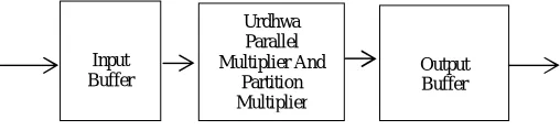
IV. PROPOSED TECHNOLOGY
As observed, 16 point DHT, involves 12 multiplications along with 42 additions. An ancient technique of vedic times called Urdhwa tiryakbhyam is used for multiplication [9, 10] along with the addition of parallel and partition multiplier with urdhawa multiplier is used. Delay and complexity are reduced to a great extent by this multiplication technique. While multiplication process, Kogge Stone adder is used in place of conventional adders which gives further enhancement in terms of speed and area occupied.
V. RESULT AND SIMULATION
A. Simulation
The simulation was performed using XILINX 14.1i and ModelSim simulator. B. Synthesis Utilization
Device utilization summary for 8-point, 16-point discrete Hartley transform along with proposed Urdhwa parallel multiplier and partition multiplier technique are shown in table III and table IV respectively.
It is observed from the table that the processing unit for 8-point DHT uses 530 slice, 940 4-input look up table (LUTs), 264 input output bounds (IOBs), 30.340 nsec maximum combination path delay using Urdhwa parallel multiplier and
Input Buffer
Urdhwa Parallel Multiplier And
Partition Multiplier
Output Buffer
path delay using partition multiplier method. It is observed from the table that the processing unit for 16-point DHT uses 530 slice, 940 4-input look up table (LUTs), 264 input output bounds (IOBs), 30.340 nsec maximum combination path delay using Urdhwa parallel multiplier and uses 385 slice, 693 4-input look up table (LUTs), 264 input output bounds (IOBs), 26.076 nsec maximum combination path delay using partition multiplier method.
Table I: Device Utilization Summary for 8-point Discrete Hartley Transform
Device Spantan-3E 3s100evq100-5
Architecture DHT using Parallel Multiplier
DHT using Partition Multiplier Method
Number of Slice 530 385
Number of 4 input LUTS 940 693
Number of IOs 264 264
Maximum Combinational Path Delay
30.340 ns 26.076 ns
Table II: Device Utilization Summary for 16-point Discrete Hartley Transform
Device Spantan-3E 3s100evq100-5
Architecture DHT using Parallel
Multiplier
DHT using Partition Multiplier Method
Number of Slice 1834 1039
Number of 4 input LUTS 3233 1843
Number of IOs 536 536
Maximum Combinational Path Delay
35.027 ns 29.547 ns
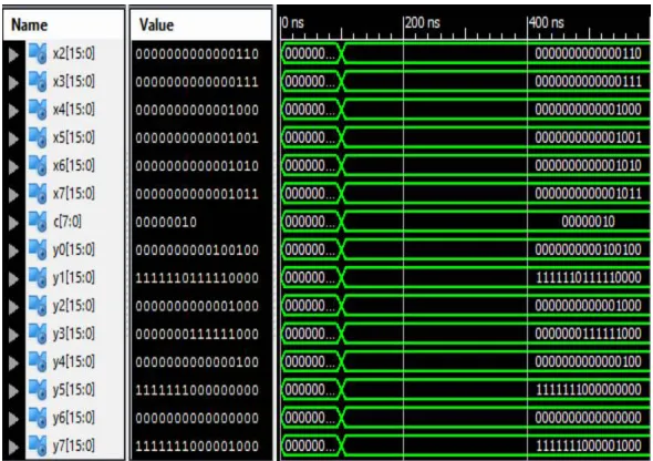
C. Resistor Transfer Level and Output Waveform
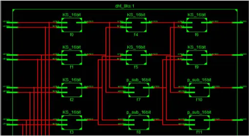
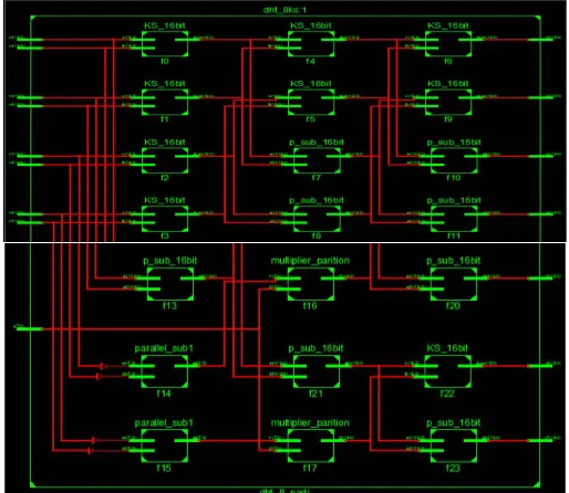
Figure 6: RTL View of 8-point DHT using Urdhwa Parallel Multiplier
Figure 8: Output Waveform of 8-point DHT D. Comparison Result
As shown in table V the maximum frequency and number of slice result are obtained for the proposed DHT using partition method algorithm and previous algorithm. From the analysis of the results, it is found that the proposed algorithm gives a superior performance as compared with previous algorithm.
Table III: Comparison of Result with Previous DHT Implementation
The proposed algorithm gives a maximum combinational path delay 26.076 ns for Spartan 3E device family as compared with 33.875 ns for previous algorithm.
VI. CONCLUSION
In order to transform a real value from time domain to real value in frequency domain, DHT is widely used for the same. It has applications in scientific, image processing, space science fields. Urdhwa Triyambakam, the most ancient technique used widely for multiplication. The key features which need to be considered are delay and area required by hardware. Here, DHT with 8×8 parallel multiplier and partition multiplier along with Kogge Stone adder which reduces the delay, area and number of slices required while computation as compared to conventional DHT computation. Among all, thesis method takes least number of slices and provides the least amount of delay.
Parameter Previous
Algorithm
DHT using Parallel Multiplier
DHT using Partition Multiplier Method
No. of Slices 673 530 385
No. of 4 input LUTs 1047 940 693
No. of bounded IOBs 264 264 264
REFERENCES
[1] G. Challa Ram and D. Sudha Rani, “Area Efficient Modified Vedic Multiplier”, 2016 International Conference Circuit, Power and Computing Technologies (ICCPCT).
[2] G. Gokhale and P. D. Bahirgonde, “Design of Vedic Multiplier using Area- Efficient Carry Select Adder”, 4th IEEE International Conference on Advances in Computing, Communications and Informatics (ICACCI-2015), Kochi, August10-13, 2015, India.
[3] G. Gokhale and Mr. S. R. Gokhale, “Design of Area and Delay Efficient Vedic Multiplier Using Carry Select Adder”, 4th IEEE International Conference on Advances in Computing, Communications and Informatics (ICACCI- 2015),Kochi, August 10-13, 2015, India.
[4] Shirali Parsai, Swapnil Jain and Jyoti Dangi, “VHDL Implementation of Discrete Hartley Transform using Urdhwa Multiplier”, 2015 IEEE Bombay Section Symposium (IBSS).
[5] Doru Florin Chiper, Senior Member, IEEE, “A Novel VLSI DHT Algorithm for a Highly Modular and Parallel Architecture”, IEEE Transactions on circuits and systems—II, VOL. 60, No. 5, May 2013.
[6] Sushma R. Huddar and Sudhir Rao, Kalpana M., “Novel High Speed Vedic Mathematics Multiplier using Compressors”, 978-1 - 4673-5090-7/13©2013 IEEE.
[7] S. S. Kerur, Prakash Narchi, Jayashree C N, Harish M Kittur and Girish V A, “Implementation of Vedic multiplier for Digital Signal Processing”, International Conference on VLSI, Communication & Instrumentation (ICVCI) 2011, Proceedings published by International Joural of Computer Applications® (IJCA), pp.1 -6.
[8] Himanshu Thapaliyal and M.B Srinivas, “VLSI Implementation of RSA Encryption System Using Ancient Indian Vedic Mathematics”, Center for VLSI and Embedded System Technologies, International Institute of Information Technology Hyderabad, India.
[9] Jagadguru Swami Sri Bharati Krishna Tirthaji Maharaja, “Vedic Mathematics: Sixteen simple Mathematical Formulae from the Veda”, Delhi (2011).
[10] Sumit Vaidya and Depak Dandekar. “Delay-power performance comparison of multipliers in VLSI circuit design”. International Journal of Computer Networks & Communications (IJCNC), Vol.2, No.4, July 2010.