Analysis of Radar Echoes using Soft Thresholding De-Noising Techniques

Analysis of Radar Echoes using Soft

Thresholding De-Noising Techniques

K.Sumiya1, N.Padmaja2, K. Bhaskar Reddy3

PG Student [DECS], Dept. of ECE, Sree Vidyanikethan Engineering College, Tirupati, Andhra Pradesh, India1 Professor, Dept. of ECE, Sree Vidyanikethan Engineering College, Tirupati, Andhra Pradesh, India2 PG Student [DECS], Dept. of ECE, Sree Vidyanikethan Engineering College, Tirupati, Andhra Pradesh, India3

ABSTRACT:In signal analysis, a lot of efforts are done to de-noise the signals well. Various techniques are used to

de-noise and improve the SNR (Signal to Noise Ratio). The Empirical Mode Decomposition (EMD) is used to extort the Intrinsic Mode functions (IMF) for LAWP (Lower Atmospheric Wind Profiler) and MST (Mesosphere, Stratosphere, Troposphere Radar signals and apply soft thresholding technique to de-noise the signals for various beam directions. All the experiments can be done with MATLAB and using signal processing tool box. Soft thresholding can de-noise the signals better than the fourier transforms and wavelet transforms. The LAWP and MST radar signals return from atmosphere are non linear and non stationary in nature and various signal de-noising techniques can be used for obtaining better results and we can see Doppler profiles of various beam directions, SNR plots and their IMF’s in results.

KEYWORDS: LAWP (Lower atmospheric wind profiler),EMD (Empirical Mode Decomposition), MST(Mesosphere,

Stratosphere, Troposphere) IMF (Intrinsic mode function), SNR( Signal to noise ratio),soft thresholding, fourier transforms and wavelet transforms..

I.INTRODUCTION

Traditional methods like fourier transforms [3] and wavelet transforms are not suitable to analyse the non linear and non stationary signals. FFT is a simplest and basic method and it requires linearity. In this method the frequency of the signal is self-determining of time, and it is also appropriate only for stationary signals.

Wavelet Transforms is another method have a major drawback is fixed basis function and it shift out the structures from chosen signal due to its precedent basis function. There is a chance that the selected mother wavelet may or may not reflect the processes which is actually present in the analyzed signal. Due to the wrong selection of wavelets which are used to associate with signal, may calculate wrong coefficient and variance. This result is misleading and it has no meaning.

II.LOWER ATMOSPHERIC WIND PROFILER (LAWP) RADAR

relatively low-cost system and it is developed in India. Hence it is very important to develop de-noising algorithms for LAWP system. LAWP system gives good resolution wind profiler parameters in all weather conditions. Atmospheric radars working in the (40-60 MHz) band has some separate advantages.

Fig 1: Block diagram of LAWP Radar

The vertical atmospheric motions can be measured at these frequencies, even during the rainfall. However, these radars have a serious constraint namely their inability to measure high-resolution winds in the first few kilometers. It probes up to about 5 km. The system should have a height motion of 100 m or better. The features of high spatial motion and fast system recovery time require operation at frequencies near 1000 MHz [8] and these wind profiler radars are very high sensitive, coherent and pulse Doppler Radars.

LAWP radar has applications beyond wind profiling. It is used for atmospheric and operational meteorology research. It can measure the complete Doppler spectrum of atmospheric targets with a time resolution on the order of 1min and a range resolution of about 100m. These LAWP data can be used to estimate the Moments, Noise Levels and UVW Computation. LAWP radar can be used to distinguish the clear-air scattering from the precipitation scattering arising from cloud and rain drops.

LAWP Radar wind profilers use either Spaced Antenna (SA) or Doppler Beam Swinging (DBS) technique for measuring the atmospheric winds. Present work uses DBS technique for measuring the atmospheric winds. Radar echoes are recorded in beam directions, viz. East, West, Zenith-x, Zenith-y, North, South directions. Here we are applying the technique of data set on 9 oct 2009.

III. EMPIRICAL MODE DECOMPOSITION

must be legitimately adjusted keeping in mind the end goal to be reliable with the exceptional qualities of the flag modes that outcome from EMD.

a. EMD Algorithm:

Given a non-stationary flag x(t) [3] , the Empirical mode strategy calculation can be compressed into taking after strides :

1. Locate the neighborhood maxima and minima of the flag then interface all the maxima and minima of flag X(t) using smooth cubic splines and acquire the upper envelope Xu(t) and the lower envelope Xl(t) separately.

2. Process the neighborhood mean esteem m1(t) = (Xu(t)+Xl(t))/2 of information X(t), subtract the mean an incentive from flag X(t) and get the distinction : h1(t)=X(t)- m1(t).

3. Accept h1(t) as new information and rehash steps(1) and (2) for k times, h1k(t)=h1(k-1)(t)- m1(t), where m1k(t) is the mean estimation of h1(k-1)(t) and h1k(t). Step(3) is ended until the subsequent information fulfills the two states of an inherent mode work, characterized as c1(t)=h1k. The lingering information r1(t) is communicated as r1(t)= X(t)- c1(t).

4. Expect r1(t) as new information and rehash steps (1),(2) and (3) and concentrate every one of the IMFs. End the filtering procedure until the nth deposit rn (t) turns out to be not as much as a foreordained number or the buildup ends up noticeably monotonic.

5. Rehash steps 1 to 4 till the leftover at no time in the future contains any helpful recurrence data. The first flag is equivalent to the whole of its IMFs. In the event that we have "n" IMFs and a last remaining rn (t), the first flag X(t) can be characterized as appeared in underneath condition (1)

X(t ) = ∑ + ---(1)

b. Intrinsic Mode Functions:

After the use of EMD if the buildup, r1 still contains data of longer period segments, then it is again regarded as the new

information and subjected to an indistinguishable filtering process from portrayed previously.

This filtering procedure can be ceased by any of the foreordained criteria: either when the part esteem cn or the deposit

rn ,turns out to be not as much as the foreordained esteem or likewise when the buildup, rn turns into a monotonic

capacity from which no more IMFs can be separated.[13] The IMF parts save enough physical sense, we need to decide a foundation for halting the filtering procedure. This should be possible by restricting the span of the Standard Deviation (SD) which can be registered from the two sequential filtering comes about as appeared in the condition (2) underneath.

SD = ∑ ( ( )( ) ( ))

( )( )

---(2) A common incentive for Standard Deviation can be set in the vicinity of 0.21 and 0.3. In the present work, we concentrate on applying the Empirical Mode Decomposition prepare on LAWP radar information to get the Intrinsic Mode Functions. At first Hard thresholding (like de-noising in Wavelets) was utilized to treat Intrinsic Mode Functions and examined for the doppler reverberate location. On watching the outcomes, Soft Threholding appeared to be suitable and was embraced for de-noising. At that point the mean clamor level was computed by Hildebrand Sekhon strategy .

IV. DENOISING

c.EMD de-noising using Thresholding:

a.) Soft Threshold b.) Hard Threshold

If Γ[τj] is a thresholding function, and τj is the threshold parameter, the threshold can be determined in different ways. Donoho and Johnstone proposed a universal threshold, τj for removing noise.

The method of soft threshold [9] is applied to process the radar data. After extracting the Intrinsic Mode functions in each range bin, de-noising techniques are employed before reconstruction of the Doppler spectra by using threshold levels.

d.Hard Thresholding:

Hard threshold removes the corresponding IMFs depending on the frequencies if τj is less than or equal to 1. The condition for

hard threshold as shown in equation (3) and (4) fj (t) = IMFj (t) If |IMFj(t)| > τj

0 If |IMFj (t)| ≤ τj ---(3)

fj (t) = IMFj(t) If |IMFj (t)| > τj

1 If |IMFj (t)| ≤ τj ---(4)

e.Soft Thresholding:

Soft thresholding process tends to shrink noise towards zero. By taking the median values of IMFs, σ˜j and τj were

calculated using equations (5),(6),and (7).

τj = ˜σj sqrt(2. loge(N)) ---(5) σ˜j = MADj / 0.6745 ---(6)

MADj = Median {|IMFj (t) −Median {IMFj (t)}|}---(7) Where σ˜j is the estimation of the noise level of the j

th

IMF (scale level) and MADj represents the absolute median deviation of the jth IMF. The soft thresholding shrinks the IMF samples by τj towards zero as follows.

ˆfj (t) = IMFj (t) − τj If IMFj (t) ≥ τj

0 If |IMFj(t)| < τj

IMFj (t) + τj If IMFj (t) ≤ −τj ---(8)

After applying soft thresholding to the IMFs, signal can be reconstructed by adding[10] all IMFs which gives de-noised signal. Similarly this procedure is applied for all the range bins. Further, three point moving average method was applied to each range and also calculated the mean noise level for each range bin and subtracted the estimated the noise level from the signal for each range bin. The results of FFT and soft thresholding shown in below figures.

V. MOMENTS CALCULATIONS

Three lower order Spectral moments (zero, first and second) and SNR are calculated by using adaptive moments method [13]. These three spectral moment represents the signal strength (power), the weighted mean Doppler shift and width of the spectrum [2-4]. The moments were calculated for the data of 9th Oct 2009 and 28th may 2009 data by using FFT and Soft Thresholding.. The expressions for the first three moments are as follows.

The 0th moment representing the total signal power is





P

M

The 1st moment representing the weighted mean Doppler shift is





f

P

M

M

(

1

/

)

---(10)

The 2nd moment representing the variance, a measure of dispersion from the mean frequency is

---(11)







i

f

M

P

M

Where m, n are the lower and upper limits of the Doppler bin of the spectral window. Pi, fi are the powers and frequencies

corresponding to the Doppler bins within the spectral window.

Signal-to-noise ratio (SNR) in dB is calculated by equation (12).

SNR















L

N

M

.

log

10

---(12)

Where N and L are the total number of Doppler bins and mean noise level respectively which on multiplication gives the total noise over the whole bandwidth.

Doppler width, which is taken to be the full width of the Doppler spectrum is calculated as:

Doppler Width



2



M



The results for two lawp data taken from NARL, Gadanki are 9 Oct 2009, 28 may 2009. De-noise the the signals by soft thresholding and also compared with FFT , original Doppler profiles and also corresponding imf’s of different beams, and also plots of the snr, power, noise Doppler width and Doppler profile and also calculate the values and tabulated for two data sets.

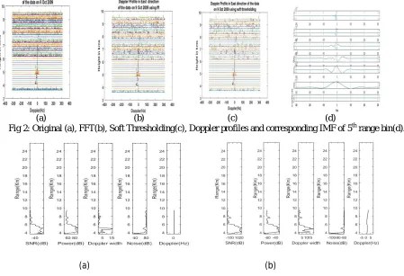
(a) (b) (c) (d)

Fig 2: Original (a), FFT(b), Soft Thresholding(c), Doppler profiles and corresponding IMF of 5th range bin(d).

(a) (b)

(c) (d)

Fig 4: Plots of SNR, power, Doppler width, noise and Doppler of FFT(c) and Soft Thresholding (d) in beam 1 (28 may 2009)

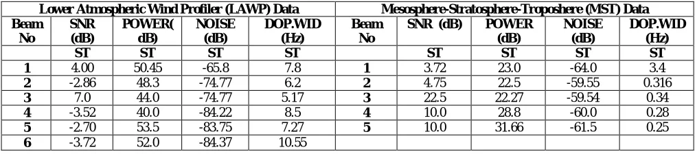
Lower Atmospheric Wind Profiler (LAWP) Data Mesosphere-Stratosphere-Troposhere (MST) Data

Beam No

SNR (dB)

POWER (dB)

NOISE (dB)

DOP.WID (Hz)

Beam No SNR (dB) POWER

(dB)

NOISE (dB)

DOP.WID (Hz)

FFT FFT FFT FFT FFT FFT FFT FFT

1 -32.1 60.5 73.33 6.125 1 -23.77 78.33 70.83 0.26

2 -42.5 72.2 72.5 5 2 -17.77 77.72 70.0 0.1

3 -34.22 66.5 64.2 3.2 3 -29.2 70.2 70.0 0.144

4 -34.0 68.125 70.0 8.22 4 -28.88 72.22 72.22 0.244

5 -34.0 66.3 71.14 4.44 5 -31.11 71.11 69.0 0.177

6 -26.11 63.5 71.8 3.03

Table 1: Avg values of SNR, power, noise, Doppler width of different beams using FFT on 9 Oct 2009(LAWP) and 28 may 2009(MST) Radar data

Lower Atmospheric Wind Profiler (LAWP) Data Mesosphere-Stratosphere-Troposhere (MST) Data

Beam No

SNR (dB)

POWER( dB)

NOISE (dB)

DOP.WID (Hz)

Beam No

SNR (dB) POWER

(dB)

NOISE (dB)

DOP.WID (Hz)

ST ST ST ST ST ST ST ST

1 4.00 50.45 -65.8 7.8 1 3.72 23.0 -64.0 3.4

2 -2.86 48.3 -74.77 6.2 2 4.75 22.5 -59.55 0.316

3 7.0 44.0 -74.77 5.17 3 22.5 22.27 -59.54 0.34

4 -3.52 40.0 -84.22 8.5 4 10.0 28.8 -60.0 0.28

5 -2.70 53.5 -83.75 7.27 5 10.0 31.66 -61.5 0.25

6 -3.72 52.0 -84.37 10.55

Table 2: Avg values of SNR, power, Doppler width, noise of different beams using Soft Thresholding on 9 Oct 2009(LAWP) and 28 may 2009 (MST) Radar data

VII. CONCLUSIONS

Doppler width plots of various beams of two data sets of LAWP and also tabulate the values. It has been observed that there is an improvement in SNR, soft thresholdng is effectively de-noise the signals

REFERENCES

[1]. Norden E. Huang, Z. Shen, and S. R. Long, M.L.Wu, E. H. Shih, Q. Zheng,C..Tung, and H. H’Liu,“The Empirical Mode Decomposition and the Hilbert Spectrum for Nonlinear and NonstationaryTimeSeries Analysis,” Proceedings of the Royal Society of London A, (1998) vol. 454,pp 903-995.

[2]. Jesmin Khan, Sharif Bhuiyan, Gregory Murphy, Mohammad Alam4, “Noise Removal from ECG Signal Using Empirical Mode Decomposition”, Aug 2014, Vol. 1 Iss. 2, PP. 45-56.

[3]. Kore Sunil N, Kore Govind Vishawanath “Adaptive ECG Noise Removal Techniques EMD and EEMD”, ISSN(Online): 2320-9801.

[4]. Jeena Joy, Salice Peter, Neetha John, “De-noising Using Soft Thresholding”, ISSN (Print) : 2320 – 3765 ISSN (Online): 2278 – 8875. [5]. P.Srinivasulu, P. Yasodha, S. N. Reddy, S.Satyanarayana and A. Jayaraman,“Simplified Active Array L-Band Radar for Atmospheric

Wind Profiling: Initial Results”, Journal of Atmospheric and Oceanic Technology, Volume 28, 1436-1447, November 2011.

[6]. Donoho, D.L.; Johnstone, I.M. “Adapting to unknown smoothness via wavelet shrinkage”, J. Amer.Statist. Assn. 1995, 90, 1200–1224. [7]. .P. Flandrin, G. Rilling, and P. Gonc¸alv`es, “Empirical mode decomposition as a filter bank,” IEEE Signal Process. Lett., vol. 11, no. 2, pp.

112–114, Feb. 2004.

[8]. P. Srinivasulu, P. Yasodha, S. N. Reddy, P. Kamaraj, T. N. Rao, S.Satyanarayana, and A. Jayaraman, “1280 MHz Active Array Radar Wind Profiler for Lower Atmosphere: System Description and Data Validation”, Journal of Atmospheric and Oceanic Technology, Volume 29, 1455-1470, October 2012.

[9]. Hildebrand, P. H., R. S. Sekhon, “Objective determination of the noise level in Doppler spectra”, J. Appl. Meteorol.Pp808-811, 1974.

[10].Z. Wu and N. E. Huang, “A study of the characteristics of white noise using the empirical mode decomposition method”. Proc. Roy. Soc London A, 2004, Vol. 460, pp. 1597-1611.

[11].J.G. Proakis and D.G. Manolakis, Digital Signal Processing: Principles, Algorithms, and Applications(3rd edition), Prentice-Hall, 1996. [12].H. Liang, Q. H. Lin, and J.D.Z. Chen, “Application of the empirical mode decomposition to the analysis of esophageal manometric data in

gastroesophageal reflux disease,” IEEE Transactions on Biomedical Engineering, vol. 52, issue. 10, pp. 1692-1701, October 2005.

[13].N.Padmaja Dr.S.Varadarajan R.Swathi, “Signal Processing Of Radar Echoes Using Wavelets And Hilbert Huang Transform”, Signal & Image Processing : An International Journal (SIPIJ) Vol.2, No.3, September 2011.

[14].G. Rilling and P. Flandrin, “One or two frequencies? the empirical mode decomposition answers,” IEEE Trans. Signal Processing, pp. 85–95, Jan. 2008.

[15].Y. Kopsinis and S.McLauglin, “Investigation and performance enhancement of the empirical mode decomposition method based on a heuristic search optimization approach,” IEEETrans. Signal Processing, pp. 1–13, Jan. 2008.

[16].Y. Kopsinis and S. McLauglin, “Improved emd using doubly iterativesifting and high order spline interpolation,” Journal on Advances of Signal processing (JASP), vol. 2008, Article ID 128293, 8 pages, 2008. doi:10.1155/2008/128293.

[17].Y. Zhang, Y. Gao, L. Wang, J. Chen, and X. Shi, “The removal of wall components in doppler ultrasound signals by using the empirica lmode decomposition algorithm,” IEEE Trans.Biomed. Eng., vol. 9, pp. 1631–1642, Sept. 2007.

[18].H. C. Huang and N. Cressie, “Deterministic/stochastic wavelet decomposition for recovery of signal from noisy data,” Technometrics, vol. 42, pp. 262–276, 2000.

[19].N. E. Huang Z. Wu, Statistical significance test of intrinsic mode functions, (in N. E. Huang and S. Shen, Hilbert-Huang Transform and Its Applications), World Scientific PublishingCompany, first edition, 2005.

[20].A. O. Boudraa and J. C. Cexus, “Denoising via empirical mode decomposition,” in ISCCSP2006, 2006.

[21].Y. Mao and P. Que, “Noise suppression and flaw detection of ultrasonic signals via empirical mode decomposition,” Russian Journal of Nondestructive Testing, vol. 43, pp. 196–203, 2007.

[22].T. Jing-tian, Z. Qing, T. Yan, L. Bin, and Z. Xiao-kai, “Hilberthuang transform for ECG de-noising,” in 1st International Conference on Bioinformatics and Biomedical Engineering (ICBBE 2007), 2007.

[23]. I. M. Johnstone and B. W. Silverman, “Wavelet threshold estimators for data with correlated noise,” J. of the Royal StatisticalSociety. Series B, vol. 59, pp. 319–351, 1997.

[24].S.Mallat, A wavelet tour of signal processing, Academic press, second edition, 1999.