Quantitative Susceptibility Imaging of Tissue Microstructure Using Ultra-High Field MRI

(1)

Electronic Thesis and Dissertation Repository

3-20-2014 12:00 AM

Quantitative Susceptibility Imaging of Tissue Microstructure

Using Ultra-High Field MRI

David A. Rudko

The University of Western Ontario

Supervisor Dr. Ravi S. Menon

The University of Western Ontario Graduate Program in Physics

A thesis submitted in partial fulfillment of the requirements for the degree in Doctor of Philosophy

Follow this and additional works at: https://ir.lib.uwo.ca/etd Part of the Medical Biophysics Commons

Recommended Citation Recommended Citation

Rudko, David A., "Quantitative Susceptibility Imaging of Tissue Microstructure Using Ultra-High Field MRI" (2014). Electronic Thesis and Dissertation Repository. 1922.

https://ir.lib.uwo.ca/etd/1922

This Dissertation/Thesis is brought to you for free and open access by Scholarship@Western. It has been accepted for inclusion in Electronic Thesis and Dissertation Repository by an authorized administrator of

(2)

QUANTITATIVE SUSCEPTIBILITY IMAGING OF TISSUE

MICROSTRUCTURE USING ULTRA-HIGH FIELD MRI

(Thesis format: Integrated Article)

by

David Alexander Rudko

Graduate Program in Physics and Astronomy

A thesis submitted in partial fulfillment of the requirements for the degree of

Doctor of Philosophy

The School of Graduate and Postdoctoral Studies The University of Western Ontario

London, Ontario, Canada

(3)

ii

This thesis has used ultra-high field (UHF) magnetic resonance imaging (MRI) to

investigate the fundamental relationships between tissue microstructure and such

susceptibility-based contrast parameters as the apparent transverse relaxation rate (R2*), the local Larmor frequency shift (LFS) and quantitative volume magnetic susceptibility

(QS). The interaction of magnetic fields with biological tissues results in shifts in the LFS

which can be used to distinguish underlying cellular architecture. The LFS is also linked

to the relaxation properties of tissues in a gradient echo MRI sequence. Equally relevant,

histological analysis has identified iron and myelin as two major sources of the LFS. As a

result, computation of LFS and the associated volume magnetic susceptibility from MRI

phase data may serve as a significant method for in vivo monitoring of changes in iron

and myelin associated with normal, healthy aging, as well as neurological disease

processes.

In this research, the cellular level underpinnings of the R2* and LFS signals were examined in a model rat brain system using 9.4 T MRI. The study was carried out using

biophysical modeling and correlation with quantitative histology. For the first time,

multiple biophysical modeling schemes were compared in both gray and white matter of

excised rat brain tissue. Suprisingly, R2* dependence on tissue orientation has not been fully understood. Accordingly, scaling relations were derived for calculating the

reversible, mesoscopic magnetic field component, R2′, of the apparent transverse relaxation rate from the orientation dependence in gray and white matter. Our results

(4)

iii

gray matter has a sinusoidal dependence on tissue orientation and a linear dependence on

the volume fraction of myelin in the tissue.

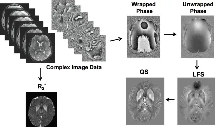
A susceptibility processing pipeline was also developed and applied to the

calculation of phase-combined LFS and QS maps. The processing pipeline was

subsequently used to monitor myelin and iron changes in multiple sclerosis (MS) patients

compared to healthy, age and gender-matched controls. With the use of QS and R2* mapping, evidence of statistically significant increases in iron deposition in sub-cortical

gray matter, as well as myelin degeneration along the white matter skeleton, were

identified in MS patients. The magnetic susceptibility-based MRI methods were then

employed as potential clinical biomarkers for disease severity monitoring of MS. It was

demonstrated that the combined use of R2* and QS, obtained from multi-echo gradient echo MRI, could serve as an improved metric for monitoring both gray and white matter

changes in early MS.

Keywords

(5)

iv

The research documented in this study would not have been possible without the

exceptional guidance, support and encouragement of a few key people. First and

foremost, I would like to thank my supervisor, Dr. Ravi Menon. His insistence on

precision, clarity and rigorous research standards remains an enduring influence. Ravi’s

insightful suggestions and knowlegeable mentoring have been particularly invaluable. He

has been an exceptional role model.

I also wish to thank Joe Gati for his continual encouragement and good-natured

advice during my work at the Center for Functional and Metabolic Mapping. As well, I

am particularly indebted to my advisory committee members, Dr. Charles McKenzie and

Dr. Tamie Poepping. They were always available, provided supportive insights and

shared their professional expertise during committee meetings.

I am especially grateful to Dr. Marcelo Kremenchutzky for his expert clinical

guidance during my observership sessions at the London Multiple Sclerosis Clinic. His

clear, concise medical diagnoses, coupled with the extensive time he spent talking with

patients, were truly exemplary. Jennifer Moussa, clinical coordinator for Dr.

Kremenchutzky, was indispensable in helping me navigate the organization and ethics

associated with the 7T MS clinical study.

My experience as a graduate student in the Medical Physics program at the

University of Western Ontario has been incredibly rewarding thanks to the stimulating

work, supportive relationships and shared challenges with fellow grad students and

co-workers at the Robarts Research Institute. Andrew Curtis was a great friend and cohort

(6)

v

and life in general helped place things in proper perspective. I would also like to thank

Igor Solovey, a software engineer in our group. His assistance with the processing

pipeline facilitated some of the reconstructions outlined in this thesis.

Most of all, though, I would like to thank both my fiancé, Sonali, and my

wonderful family for their constant understanding, unconditional support and ongoing

(7)

vi

The contributions of the authors to each of the manuscripts documented in this thesis are

outlined below:

Mr. David Rudko, in the capacity of doctoral candidate, outlined the objectives,

developed the methodology, conducted the experiments, acquired and analyzed the data,

and developed the software employed for data analysis. He also wrote and prepared the

manuscripts for publication. Dr. Martyn Klassen, in the capacity of co-author for the first

manuscript (presented in Chapter 4), assisted the primary author in data analysis. Ms.

Sonali de Chickera, in the capacity of co-author for the first manuscript, prepared,

sectioned, and stained tissue sections for histological analysis. She also assisted in

generating figures for publication. Mr. Greg Dekaban, in the capacity of co-author for the

first manuscript, contributed histological staining reagents and helped with editing.

Dr. Marcelo Kremenchutzky, in the capacity of co-author of the second

manuscript (presented in Chapter 5), assisted in protocol planning for the 7 T MS study.

He is listed as a principal investigator for the human ethics protocol associated with this

study. Mr. Joseph Gati, in the capacity of co-author for both manuscripts, assisted with

scan protocol development. Dr. Ravi Menon, the candidate’s supervisor and co-author of

both manuscripts, provided guidance, mentorship, and supervision for both projects. He

is also listed as a principal investigator for the human ethics protocol used in the 7 T MS

(8)

vii

List of Figures

Figure 2.1 Classical representation of the nuclear magnetization…..…..………18

Figure 2.2 Magnetization under the influence of an RF pulse with flip angle θ = γ B1t along the x′-axis………..………..………...18

Figure 2.3 Schematic representation of the magnetization in the rotating frame...……….………...19

Figure 2.4 Ideal time and Fourier domain representations of the NMR signal…...………....……..21

Figure 2.5 NMR signal for compounds whose protons experience different local magnetic fields……….……….…..21

Figure 2.6 NMR signal for a sample of pure water subject to T2-relaxation……...………..………..………..………...22

Figure 2.7 Linear relationship between slice thickness and RF pulse bandwidth (Δω)………..………..………..………....23

Figure 2.8 Fourier relationships between the frequency domain signal and image domain signal in MRI……….………24

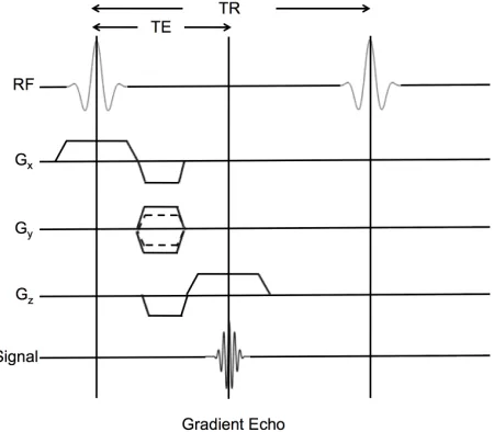
Figure 2.9 Pulse sequence diagram illustrating a typical gradient echo imaging sequence………... 25

Figure 2.10 Schematic representation of gradient recalled echo signal decay and measurement using a multi-echo gradient echo sequence……… 27

Figure 3.1 SHARP background filter convolution kernels with varying radii………..….41

Figure 3.2 SHARP filtered LFS maps generated using an increasing kernel radius………42

Figure 3.3 QSM dipole convolution function………...….……….44

Figure 3.4 Spatial priors used in calculation of QS maps…………..……….45

Figure 3.5 Full susceptibility processing pipeline……….46

(15)

xiv

changes observed in grey and white matter as a function of fiber orientation………….………..65 Figure 4.3 Comparison between Δχdipole and ΔχGLModel……….……...73

Figure 4.4 R2* and quantitative susceptibility correlations with Fe3+ iron………..76 Figure 4.5 Correlation between linear model constants and myelin OD...78

Figure 5.1 Representative MR image contrasts employed in the 7 T MS imaging study………...………...93 Figure 5.2 Standard space, susceptibility-based MRI contrast………...…..94

Figure 5.3 Representative sub-cortical nuclei segmentations.….……….95

Figure 5.4 Correlations between R2*_{and QS and EDSS scale in MS} patients……….96 Figure 5.5 R2*_{-based, axial Z-score maps depicting disease-related changes...99} Figure 5.6 QS-based, axial Z-score maps depicting disease-related changes……...………103 Figure 5.7 Changes in relative magnetic susceptiblity as a function of age……….……….104 Figure 5.8 Relationship between volume occupied by significant negative Z-scores and EDSS………...………..106 Figure 6.1 Temporal evolution of the mean R2* _{and LFS signal within RRMS} white matter lesions over the course of the first year of the longitudinal MS imaging study. ………..128 Figure 6.2. Representative longitudinal images from a select patient with RRMS……..………...129 Figure 6.3. Cropped and enlarged lesions as visualized by UHF MRI………...130

(16)

xv

List of Appendices

(17)

xvi

ΔB magnetic field shift

CIS clinically isolated syndrome CNS central nervous system

EDSS extended disability status scale

fext external/background Larmor frequency shift

fint internal/local, tissue-specific Larmor frequency shift

ftot total Larmor frequency shift integrated over the imaging volume fL local (Larmor) frequency shift

GM gray matter

GRE gradient recalled echo

LFS local (Larmor) frequency shift MS multiple sclerosis

OD optical density

qMRI quantitative magnetic resonance imaging QSM quantitative susceptibility mapping R2 transverse relaxation rate

R2∗ effective transverse relaxation rate

R2’ reversible component of the effective transverse relaxation rate ROI region of interest

RRMS relapsing-remitting multiple sclerosis SNR signal-to-noise ratio

T1 longitudinal relaxation rate T2 transverse relaxation rate

TE echo time

TR repetition time

UHF ultra-high field

WM white matter

θ image phase

(18)

xvii

Scope of Thesis

The following is a brief overview of each chapter contained in this thesis. Chapter One

introduces the principles, methodologies and relevance of the research studies composing

the thesis. The second chapter discusses the underlying background of MRI physics,

signal acquisition and phase processing necessary for understanding relaxometry and

susceptibility mapping. A processing pipeline for multi-echo, gradient echo-based

quantification of tissue magnetic properties (R2*_{, LFS, and}_{Δχ) is then examined in the}

third chapter.

Chapter Four derives from a manuscript published in the Proceedings of the

National Academy of Sciences of the United States of America (Rudko et al., PNAS,

Jan 7, 2014, 111(1), E159-167). It presents a fundamental research study utilizing

combined R2*, LFS and QS mapping with multi-echo, gradient echo MRI at high field and ultra-high resolution. Multiple biophysical modeling schemes are compared for the

first time in both gray and white matter for excised rat brain tissue.

Chapter Five derives from a manuscript accepted for publication in the journal,

Radiology (Rudko et al., Radiology, manuscript #RAD-13-2475). It highlights a 7 T

imaging study using whole-brain, quantitative Δχ and R2*_{mapping for simultaneous}

monitoring of iron deposition and demyelinating processes in MS patients. For the first

time, voxel based morphometry is combined with generalized linear model (GLM)

analysis to identify whole brain differences between patients and controls. The sixth and

final chapter briefly summarizes the research carried out for this thesis. It also suggests

ways of extending this research, with an emphasis on both technical developments and

(19)

Chapter 1 Introduction

The Prize is the pleasure of finding things out. – Richard Feynman, Quantum Man

Over the last four decades, magnetic resonance imaging (MRI) has made dramatic

progress as a non-invasive imaging modality for evaluating human tissue properties.

Advanced technological breakthroughs in MRI now enable more accurate assessment of

both the structure and function of many human organ systems. Not only is MRI being

used to diagnose a wide range of disease processes, it is also being applied to such

diverse research areas as the study of heart valve abnormalities (1), functional brain

activation (2) and autoimmune cell tracking (3).

Fundamentally, MRI uses a strong external magnetic field to generate a bulk

magnetization in the hydrogen nuclei of the human body. When these nuclei are excited

by a radiofrequency (RF) pulse, an MR signal can be detected by a receiver coil. By

adding spatially-varying, linear magnetic field gradients, images can then be

reconstructed which represent the radiofrequency signal emitted from tissues (4). For

standard MRI techniques at clinical field strengths of 1.5 and 3 Tesla (T), the

radiofrequency signal is primarily a measure of the nuclear magnetization properties of

water protons. However, in ultra-high field MRI (UHF MRI, B0 ≥ 7 T), the interaction

between the external magnetic field and the orbital electrons in biological molecules also

leads to an appreciable increase in the Larmor resonance frequency experienced by water

protons (5). This frequency perturbation can be related to the concentration of

(20)

In any MRI scan, the specific physical characteristics of tissue being visualized

depend on how the magnetic field is modulated during the acquisition process (9). Since

the acquisition consists of a repetitive cycle of varying magnetic field gradients and RF

pulses, the tissue magnetization undergoes a concomitant series of repetitive changes.

Essentially, the magnetization is perturbed from its natural state and then allowed to

recover to equilibrium through a process known as relaxation. This process provides the

basic contrast in MRI. The differential relaxation rates of tissues result in relative signal

differences observed in an image (10). In the section that follows, the sensitization of the

MRI signal to different tissue relaxation properties is outlined in more detail and related

to qMRI – a significant topic of discussion in this thesis.

1.1 Sensitizing the MRI signal to tissue properties

A pivotal improvement of MRI compared to other diagnostic imaging techniques such as

x-ray computed tomography (CT), positron emission tomography (PET), ultrasound and

optical imaging, is its ability to sensitize the signal to different properties of biological

tissue (10). The MRI signal is flexible enough to reflect such biophysical quantities as

tissue-specific nuclear relaxation rates (longitudinal relaxation rate: T1, transverse

relaxation rate: T2, or effective transverse relaxation rate: T2*_{), rate of blood flow (11),} blood oxygenation (12), water molecule self-diffusion (13), as well as tissue magnetic

and electrical properties (7, 14).

The T1 or T2–weighted contrast obtained in standard MRI methods is controlled

through the adjustment of pulse sequence timing parameters such as the duration between

(21)

results in qualitative differences in signal intensity. For example, with an external

magnetic field strength of 3 T, if contrast between gray and white matter in the human

brain is desired, one can exploit the differences in either T1 (white matter = 1100 ms, gray

matter = 1800 ms) or T2 (white matter = 70 ms , cortical gray matter = 100 ms) relaxation

characteristics of brain tissue (15).

Because of its flexibility in generating contrast, MRI is used clinically by

radiologists to confirm many soft tissue neurological disorders. However, the standard

T1- and T2-weighted images employed by radiologists do not provide true quantitative

metrics of tissue composition. They only identify relative differences in nuclear

relaxation properties (4). This is problematic when seeking to relate the MRI signal to

underlying cellular-level changes associated with either disease or normal, healthy aging.

To make MRI more predictive of underlying biology, qMRI methods have been

developed. For a qMRI parameter to be effective, it must be (i) reproducible, (ii) accurate

and (iii) specific to underlying cellular architecture (16). Reproducibility reflects the

magnitude of random errors that occur from one scan session to the next. Generally, these

should be significantly less than the natural variation of the qMRI parameter itself.

Accuracy reflects how closely a measurement is to the true value. Specificity reflects how

closely the change in the qMRI parameter reflects the change in biology of the tissue.

Two frequently employed qMRI techniques are T1 and T2 relaxometry (16). With

these two methods, specific magnetic field gradients and RF pulse combinations are used

to probe the relaxation of nuclear magnetization over time. A quantitative value of T1 or

T2 can then be assigned to each location in the brain. Relaxometry has proven valuable in

(22)

multiple sclerosis (MS) (18). However, T1 and T2 relaxometry require long acquisition

times and are usually not suitable for whole-brain imaging.

This thesis examines the use of three magnetic susceptibility-based qMRI

parameters acquired using a time-efficient, multi-echo, gradient echo sequence: apparent

transverse relaxation rate (R2*), local Larmor frequency shift (LFS) and volume magnetic susceptibility (∆χ). In all computations, standard error analysis methods are employed to

identify accuracy. In the following section, the susceptibility-based MRI parameters are

described in further detail.

1.2 Ultra-High Field (UHF) MRI and its applications to susceptibility-induced

contrast

Currently, MRI scanners at high (≥ 3 T) and ultra high-field (UHF, ≥ 7 T) offer improved

signal-to-noise ratio (SNR) and increased spatial resolution compared to standard clinical

imaging at 1.5 T. UHF MRI allows visualization of smaller structures in the human brain,

including cortical folding patterns (19) and venous vasculature organization (20). A

further advantage of UHF MRI is its increased magnetic susceptibility contrast,

particularly useful in functional MRI (fMRI) (21) and superparamagnetic iron-oxide

nano-particle (SPIO) tracking (22-24). Such applications employ the magnitude of the

complex MRI signal but disregard the phase. Recently however, it has been demonstrated

that with proper processing, the contrast observed in the MRI phase is sensitive to

relative concentration differences of such important biological substrates as myelin and

iron (6, 25).

(23)

differences in magnetic susceptibility between neighbouring tissues result in

perturbations of the local magnetic field (26). These perturbations give rise to a

detectable shift in the LFS, which is measurable through the complex image phase.

Notably, the linear increase in magnetic susceptibility-induced field perturbations in UHF

MRI results in higher signal-to-noise ratio (SNR) and improved contrast at higher B0

fields for phase imaging (27). Once the image phase has been unwrapped and background

magnetic field contributions have been removed, an estimate of tissue specific magnetic

susceptibility properties may be computed (7, 28, 29). The magnetic susceptibility is

calculated through a field-to-source inverse problem known as Quantitative Susceptibility

Mapping (QSM), which reveals anatomical features in the brain with unprecedented

quality. QSM also allows quantitative characterization of deep gray matter structures (7,

30), brain tumours (31) , and sub-cortical iron increases in MS (32).

Presently, the clinical applicability of QSM is hampered by challenges associated

with proper phase processing and interpretation of the QS signal (7). Numerical

instabilities in the field-to-source inverse calculation can result in streaking or blurring

artifacts which complicate quantitation (33). As well, the quality of QS maps critically

depends on the accuracy of the measured image phase. Incorrect phase values due to

blood flow, low SNR, or incomplete/inaccurate phase unwrapping produce significant

non-local artifacts (6). Several solutions to these issues are addressed in this thesis, as

well as the application of QSM in conjunction with R2* mapping to underlying tissue biology. Additionally, the clinical applicability for MS monitoring using combined

(24)

1.3 Application of UHF MRI to multiple sclerosis

UHF, susceptibility-based MRI of multiple sclerosis constitutes one of the major chapters

in this thesis. Accordingly, a brief overview follows of (i) the clinical symptoms and

pathophysiology of MS and (ii) the clinical monitoring of MS using UHF MRI.

1.3.1 Clinical symptoms and pathophysiology of MS

MS is a chronic, inflammatory disease of the central nervous system (CNS)

characterized by a varied and unpredictable time course (34). It is the most common

neurological disease affecting young adults in Canada (35, 36). Although the specific

cause is unknown, it appears to involve both genetic susceptibility and triggers such as a

virus, a dysregulated metabolism or environmental factors (37, 38). In most patients, MS

consists of initial episodes of reversible neurological deficit followed by progressive

deterioration, which can become severe and result in early death (34). Evolution of the

disease produces a spectrum of clinical features that may include motor weakness,

sensory and gait disturbances, vision loss and cognitive changes (34).

Several MS disease sub-types have been characterized. These are determined on

the basis of such clinical criteria as frequency of relapses, time to disease progression,

and lesion development (39). The major MS sub-types include: relapsing-remitting MS

(RRMS, approximately 85% of cases), primary progressive MS (PPMS, approximately

10% of cases) and progressive-relapsing MS (PRMS, about 5% of cases) (34). RRMS is

characterized by unpredictable relapses followed by months to years of remission. A

fourth major sub-type, secondary progressive MS (SPMS), occurs for approximately 65%

of those with initial RRMS and is defined by a progressive neurologic decline between

(25)

experience no remission and symptoms steadily worsen (34). PPMS patients have steady

neurologic decline from the onset, superimposed with attacks (34, 39).

The hallmark pathophysiology of MS is damage to myelin, axons and

oligodendrocytes (37). This occurs through a multistep mechanism involving sequential

inflammation, demyelination and neurodegeneration (34). The specific autoimmune

targets are believed to be cellular components of the CNS normally inaccessible due to

their location behind the blood–brain barrier. During disease initiation, entry of

autoimmune cells (T-cells, B-cells and monocytes) through the blood brain barrier is

triggered by cytokine and chemokine signals (37). Once within the CNS, T-cells are

stimulated and retained there by resident microglia, which present antigen receptor sites

to the T-cells. Microglia are also involved in clearing away myelin debris. This results in

further T-cell/lymphocyte infiltration (34). Concurrent with the initial autoimmune

response, the inflammatory infiltrate in white matter lesions eventually includes

macrophages at the lesion centre. These are principally responsible for myelin digestion

(37, 38).

The trigger for the T-cell mediated autoimmune attack in MS is unclear.

However, it is recognized that MS consists of repeated attacks on both myelin and

oligodendrocytes via an inflammatory cascade activated repeatedly over time. The

existing knowledge of the interconnected cellular components in the cascade has already

been used to create targeted therapies aimed at reducing progression (37, 40). From an

MRI standpoint, targeted imaging of these cellular components utilizing, for example,

iron-labeled cellular MRI (23), represents a promising avenue for monitoring critical

(26)

1.3.2 UHF MRI of MS

Conventional MRI employing standard T1- and T2-weighted imaging plays a key role in diagnosing MS (41). However, neither lesion load or lesion volume derived from these standard sequences have correlated well with clinical symptoms and scoring scales

(42). In addition, standard MRI findings have not demonstrated significant predictive

power for identifying disease progression (39). Post-mortem histopathology has revealed

the inability of standard MRI to visualize no more than a subset of the actual lesions and

damage (43).

Standard MRI pulse sequences used for monitoring MS, such as T2-weighted fast spin echo (FSE) and fluid-attenuated inversion recovery (FLAIR), visualize only

two-thirds of histopathologically detectable white matter (WM) lesions and less than

one-tenth of cortical grey matter (GM) lesions (44). Moreover, the standard sequences are

insensitive to damage in normal-appearing white matter, which is known to have a

significant role in the onset of MS (45, 46). In contrast, susceptibility-based UHF MRI

techniques, including the LFS and QS mapping methods detailed in this thesis,

potentially offer more accurate visualization of early myelin changes in gray and white

matter not visualized on standard MRI contrasts (6, 7). This is because QSM measures

both the nuclear magnetization and the accompanying magnetic susceptibility in an

imaging voxel (47). In white matter, these physical parameters are specific to the

composition of myelin, since myelin is magnetized by an amount proportional to the

magnetic susceptibility of phospholipid molecules in the myelin bilayers. Consequently,

by using UHF MRI, QSM detects an intrinsic property that may be more closely linked

to demyelination than such other methods as T2-based relaxometry or diffusion MRI

measurements of fractional anisotropy.

Equally significant, depicting MS gray matter pathology using MRI directly

(27)

damage may serve as an improved biomarker for MS monitoring (48). Indeed, UHF T2*– weighted MRI using 2D gradient echo imaging has already demonstrated an improved

sensitivity for detecting gray matter lesions in vivo at 7 T (48). T2*–weighted MRI has also been used to monitor the accumulation of non-haeme iron in sub-cortical gray matter

(30, 32, 49). Iron in sub-cortical gray matter is essential for normal neuronal metabolism,

including mitochondrial energy generation and myelination. However, excessive levels

may exert oxidative stress and result in cell death. When excess iron is present,

incomplete chelation or storage results in iron catalyzing the production of hydroxyl

radicals. The production of such radicals may trigger protein denaturation, damage to

DNA or oxidation of phospholipid membranes (50). As result, monitoring the

accumulation of non-haeme iron in the basal ganglia and linking this to clinical disability

is a major area of interest in UHF MRI of MS. It is a primary focus in the fifth chapter of

this thesis.

Several qMRI metrics, including T2, T2*, magnetic field correlation (MFC) and QSM have been proposed for monitoring basal ganglia iron in vivo. In this thesis, two of

these metrics, T2*_{and QSM, are examined. Recent research has demonstrated that the} apparent transverse relaxation rate (R2* = 1/ T2*) correlates well with basal ganglia iron (27). Regional values of R2* differ significantly between CIS patients (n = 32) and MS patients (n = 37) (51). This suggests R2* relaxometry may be a useful tool for evaluating differential iron deposition between MS disease groups. Further, it may prove helpful for

clarifying whether regional iron accumulation contributes to MS pathology or merely

reflects an epiphenomenon.

(28)

associated with normal aging (52) and MS (32) in basal ganglia structures compared to

R2*. This increased sensitivity results from the ability of QS to measure the mean magnetic field perturbation in a voxel, as opposed to the signal relaxation of protons in

water molecules (25). The mean magnetic field perturbation can then be directly linked to

the amount of iron (52). However, relaxometric measures such as R2* are not specific to the mean magnetic field. Rather, they measure the effect of intra-voxel susceptibility

gradients on phase dispersion of relaxing protons (53). In this thesis, the relative

sensitivities of R2* _{and QS to iron accumulation in MS are evaluated as clinically relevant} biomarkers.

The second chapter examines the underlying background of MRI physics, signal

acquisition and phase processing necessary for understanding relaxometry and

susceptibility mapping. For a complete overview of all chapters, refer to the ‘Scope of

(29)

1.4 References

1. Masci, P. G., S. Dymarkowski, and J. Bogaert. 2008. Valvular heart disease: what does cardiovascular MRI add? Eur Radiol 18: 197-208.

2. Matthews, P. M., and P. Jezzard. 2004. Functional magnetic resonance imaging. Journal of Neurology, Neurosurgery & Psychiatry 75: 6-12.

3. Bonetto, F., M. Srinivas, A. Heerschap, R. Mailliard, E. T. Ahrens, C. G. Figdor, and I. J. de Vries. 2011. A novel (19)F agent for detection and quantification of human dendritic cells using magnetic resonance imaging. Int J Cancer 129: 365-373.

4. Haacke, E. M., R. W. Brown, M. R. Thompson, and R. Venkatesan. 1999. Magnetic resonance imaging: physical principles and sequence design. Wiley-Liss New York:

5. Lee, J., K. Shmueli, M. Fukunaga, P. van Gelderen, H. Merkle, A. C. Silva, and J. H. Duyn. 2010. Sensitivity of MRI resonance frequency to the orientation of brain tissue microstructure. Proc Natl Acad Sci U S A 107: 5130-5135.

6. Schweser, F., K. Sommer, A. Deistung, and J. R. Reichenbach. 2012. Quantitative susceptibility mapping for investigating subtle susceptibility variations in the human brain. Neuroimage 62: 2083-2100.

7. Schweser, F., A. Deistung, B. W. Lehr, and J. R. Reichenbach. 2011. Quantitative imaging of intrinsic magnetic tissue properties using MRI signal phase: an approach to in vivo brain iron metabolism? Neuroimage 54: 2789-2807.

8. Liu, C., W. Li, G. A. Johnson, and B. Wu. 2011. High-field (9.4 T) MRI of brain dysmyelination by quantitative mapping of magnetic susceptibility. Neuroimage 56: 930-938.

9. Lufkin, R., W. L. Davis, and A. G. Osborn. 1993. Overview of MR imaging modalities. J Comput Assist Tomogr 17 Suppl 1: S24-9.

10. Plewes, D. B., and W. Kucharczyk. 2012. Physics of MRI: a primer. J Magn Reson Imaging 35: 1038-1054.

(30)

12. Ogawa, S., T. M. Lee, A. R. Kay, and D. W. Tank. 1990. Brain magnetic resonance imaging with contrast dependent on blood oxygenation. Proc Natl Acad Sci U S A 87: 9868-9872.

13. Basser, P. J., and D. K. Jones. 2002. Diffusion-tensor MRI: theory, experimental design and data analysis - a technical review. NMR Biomed 15: 456-467.

14. Tuch, D. S., V. J. Wedeen, A. M. Dale, J. S. George, and J. W. Belliveau. 2001. Conductivity tensor mapping of the human brain using diffusion tensor MRI. Proceedings of the National Academy of Sciences 98: 11697-11701.

15. Stanisz, G. J., E. E. Odrobina, J. Pun, M. Escaravage, S. J. Graham, M. J. Bronskill, and R. M. Henkelman. 2005. T1, T2 relaxation and magnetization transfer in tissue at 3T. Magn Reson Med 54: 507-512.

16. Tofts, P. S., and E. P. G. H. Du Boulay. 1990. Towards quantitative measurements of relaxation times and other parameters in the brain. Neuroradiology 32: 407-415. 17. Barnes, D., W. I. McDonald, G. Johnson, P. S. Tofts, and D. N. Landon. 1987.

Quantitative nuclear magnetic resonance imaging: characterisation of experimental cerebral oedema. Journal of Neurology, Neurosurgery & Psychiatry 50: 125-133. 18. Kidd, D., G. J. Barker, P. S. Tofts, A. Gass, A. J. Thompson, W. I. McDonald, and

D. H. Miller. 1997. The transverse magnetisation decay characteristics of longstanding lesions and normal-appearing white matter in multiple sclerosis. Journal of neurology 244: 125-130.

19. Fischl, B. 2012. FreeSurfer. Neuroimage 62: 774-781.

20. Budde, J., G. Shajan, J. Hoffmann, K. Ugurbil, and R. Pohmann. 2011. Human imaging at 9.4 T using T(2) *-, phase-, and susceptibility-weighted contrast. Magn Reson Med 65: 544-550.

21. Geissler, A., F. P. Fischmeister, G. Grabner, M. Wurnig, J. Rath, T. Foki, E. Matt, S. Trattnig, R. Beisteiner, and S. D. Robinson. 2013. Comparing the Microvascular Specificity of the 3- and 7-T BOLD Response Using ICA and Susceptibility-Weighted Imaging. Front Hum Neurosci 7: 474.

(31)

23. Rad, A. M., A. S. Arbab, A. S. M. Iskander, Q. Jiang, and H. Soltanian-Zadeh. 2007. Quantification of superparamagnetic iron oxide (SPIO)-labeled cells using MRI. Journal of Magnetic Resonance Imaging 26: 366-374.

24. Heyn, C., C. V. Bowen, B. K. Rutt, and P. J. Foster. 2005. Detection threshold of

single SPIO-labeled cells with FIESTA. Magnetic resonance in medicine 53: 312-320.

25. Deistung, A., A. Schafer, F. Schweser, U. Biedermann, R. Turner, and J. R. Reichenbach. 2013. Toward in vivo histology: a comparison of quantitative susceptibility mapping (QSM) with magnitude-, phase-, and R2*-imaging at ultra-high magnetic field strength. Neuroimage 65: 299-314.

26. Schenck, J. F. 1996. The role of magnetic susceptibility in magnetic resonance imaging: MRI magnetic compatibility of the first and second kinds. Medical physics 23: 815.

27. Yao, B., T. Q. Li, P. Gelderen, K. Shmueli, J. A. de Zwart, and J. H. Duyn. 2009. Susceptibility contrast in high field MRI of human brain as a function of tissue iron content. Neuroimage 44: 1259-1266.

28. de Rochefort, L., R. Brown, M. R. Prince, and Y. Wang. 2008. Quantitative MR susceptibility mapping using piece-wise constant regularized inversion of the magnetic field. Magn Reson Med 60: 1003-1009.

29. de Rochefort, L., T. Liu, B. Kressler, J. Liu, P. Spincemaille, V. Lebon, J. Wu, and Y. Wang. 2010. Quantitative susceptibility map reconstruction from MR phase data using bayesian regularization: validation and application to brain imaging. Magn Reson Med 63: 194-206.

30. Lebel, R. M., A. Eissa, P. Seres, G. Blevins, and A. H. Wilman. 2012. Quantitative high-field imaging of sub-cortical gray matter in multiple sclerosis. Mult Scler 18: 433-441.

(32)

32. Langkammer, C., T. Liu, M. Khalil, C. Enzinger, M. Jehna, S. Fuchs, F. Fazekas, Y. Wang, and S. Ropele. 2013. Quantitative susceptibility mapping in multiple sclerosis. Radiology 267: 551-559.

33. Reichenbach, J. R. 2012. The future of susceptibility contrast for assessment of anatomy and function. Neuroimage 62: 1311-1315.

34. Compston, A., and A. Coles. 2008. Multiple sclerosis. Lancet 372: 1502-1517. 35. Poppe, A. Y., C. Wolfson, and B. Zhu. 2008. Prevalence of multiple sclerosis in

Canada: a systematic review. Can J Neurol Sci 35: 593-601.

36. Beck, C. A., L. M. Metz, L. W. Svenson, and S. B. Patten. 2005. Regional variation of multiple sclerosis prevalence in Canada. Mult Scler 11: 516-519.

37. Ontaneda, D., M. Hyland, and J. A. Cohen. 2012. Multiple sclerosis: new insights in pathogenesis and novel therapeutics. Annual Review of Medicine 63: 389-404. 38. Sospedra, M., and R. Martin. 2005. Immunology of multiple sclerosis. Annu Rev

Immunol 23: 683-747.

39. Ceccarelli, A., R. Bakshi, and M. Neema. 2012. MRI in multiple sclerosis: a review of the current literature. Curr Opin Neurol 25: 402-409.

40. Rice, C. M., K. Kemp, A. Wilkins, and N. J. Scolding. 2013. Cell therapy for multiple sclerosis: an evolving concept with implications for other neurodegenerative diseases. Lancet 382: 1204-1213.

41. Polman, C. H., S. C. Reingold, B. Banwell, M. Clanet, J. A. Cohen, M. Filippi, K. Fujihara, E. Havrdova, M. Hutchinson, and L. Kappos. 2011. Diagnostic criteria for multiple sclerosis: 2010 revisions to the McDonald criteria. Annals of neurology 69: 292-302.

42. Filippi, M., M. A. Rocca, N. De Stefano, C. Enzinger, E. Fisher, M. A. Horsfield, M. Inglese, D. Pelletier, and G. Comi. 2011. Magnetic resonance techniques in multiple sclerosis: the present and the future. Arch Neurol 68: 1514-1520.

(33)

44. Geurts, J. J., L. Bo, P. J. Pouwels, J. A. Castelijns, C. H. Polman, and F. Barkhof. 2005. Cortical lesions in multiple sclerosis: combined postmortem MR imaging and histopathology. AJNR Am J Neuroradiol 26: 572-577.

45. Rudick, R. A., J. C. Lee, K. Nakamura, and E. Fisher. 2009. Gray matter atrophy correlates with MS disability progression measured with MSFC but not EDSS. J Neurol Sci 282: 106-111.

46. Moraal, B., C. Pohl, B. M. Uitdehaag, C. H. Polman, G. Edan, M. S. Freedman, H. P. Hartung, L. Kappos, D. H. Miller, X. Montalban, V. Lanius, R. Sandbrink, and F. Barkhof. 2009. Magnetic resonance imaging predictors of conversion to multiple sclerosis in the BENEFIT study. Arch Neurol 66: 1345-1352.

47. Li, W., B. Wu, A. V. Avram, and C. Liu. 2012. Magnetic susceptibility anisotropy of human brain in vivo and its molecular underpinnings. Neuroimage 59: 2088-2097.

48. Mainero, C., T. Benner, A. Radding, A. van der Kouwe, R. Jensen, B. R. Rosen, and R. P. Kinkel. 2009. In vivo imaging of cortical pathology in multiple sclerosis using ultra-high field MRI. Neurology 73: 941-948.

49. Ropele, S., W. de Graaf, M. Khalil, M. P. Wattjes, C. Langkammer, M. A. Rocca, A. Rovira, J. Palace, F. Barkhof, M. Filippi, and F. Fazekas. 2011. MRI assessment of iron deposition in multiple sclerosis. J Magn Reson Imaging 34: 13-21.

50. Nunez, M. T., P. Urrutia, N. Mena, P. Aguirre, V. Tapia, and J. Salazar. 2012. Iron toxicity in neurodegeneration. Biometals 25: 761-776.

51. Khalil, M., C. Langkammer, S. Ropele, K. Petrovic, M. Wallner-Blazek, M. Loitfelder, M. Jehna, G. Bachmaier, R. Schmidt, C. Enzinger, S. Fuchs, and F. Fazekas. 2011. Determinants of brain iron in multiple sclerosis: a quantitative 3T MRI study. Neurology 77: 1691-1697.

52. Bilgic, B., A. Pfefferbaum, T. Rohlfing, E. V. Sullivan, and E. Adalsteinsson. 2012. MRI estimates of brain iron concentration in normal aging using quantitative susceptibility mapping. Neuroimage 59: 2625-2635.

(34)

Chapter 2 Underlying Sources of MRI Contrast and Signal Formation

I canna’ change the laws of physics, Captain! – Scottie, head engineer in Star Trek

To provide a brief background for the discussion of transverse relaxometry, LFS and QS

mapping that follows, this chapter considers the fundamental sources of the MRI contrast

and signal formation. It is partitioned into four sections. The first section describes the

physics of MRI signal formation under the influence of a strong external magnetic field

and radiofrequency (RF) pulse perturbations. The Bloch equations are then introduced as

the mathematical model describing the time-evolution of the MRI signal. This is followed

by a discussion of the basics of MR image reconstruction. Lastly, an introductory

examination of susceptibility mapping provides a background for the phase processing

pipeline presented in Chapter three.

2.1 Underlying sources of the MRI signal

In an external magnetic field such as the one produced by a superconducting MRI

magnet, atomic nuclei can be treated as magnetic dipoles possessing a magnetic moment,

µ, and an angular momentum, L. These two parameters are related accordingly (1):

[2.1]

where γ is the gyromagnetic ratio which is specific to the nucleus of interest. The most common nucleus to be imaged in MRI is that of hydrogen bonded to oxygen in water.

(35)

single positively charged proton and a negatively charged electron bound by the Coulomb

electromagnetic field (2). Under the influence of the external field of the MRI magnet,

the proton experiences a torque (1),

_[2.2]

which can be related to the nuclear spin angular momentum by the equation (3):

[2.3]

Equation [2.3] describes the time evolution of the nuclear magnetization (M→) and forms the basis for the MRI Bloch equation - a first-order, linear differential equation describing

the magnetization dynamics (3):

[2.4]

In equation [2.4], Bext represents the combination of the static magnetic field and both the magnetic field gradients (G) and RF (B1) fields (4):

→Bext=B0k ∧

+ γG→⋅→rk∧ + B_1x∧i + B_1y∧j _[2.5] Typically, the Bloch equation is written with respect to a particular reference frame, the

most familiar of which is the frame rotating in relation to the z-axis of the scanner

coordinate system at the Larmor frequency. In this frame, the external magnetic field

becomes (4):

→Brot= →

Bext−B0k ∧

=γG→⋅→rk∧ + B_1x∧i + B_1y∧j _[2.6] Evaluating the Bloch equations in this reference frame is equivalent to stopping the free

(36)

pulses and gradients. The rotating reference frame is described pictorially as follows:

Figure 2.1: (a) Classical representation of the nuclear magnetization vector, aligned along the magnetic field in the static reference frame. (b) Schematic representation of the

reference rotating about the z-axis at the Larmor resonance frequency, (ω), of

on-resonant spins.

The primed coordinates (x′, y′ and z′) in figure 2.1 indicate the axes are rotating about the

z-axis at the Larmor frequency. During an MRI experiment, for signal to be detected by a

receiver coil, the magnetization vector must be rotated into the transverse (x′y′) plane (3).

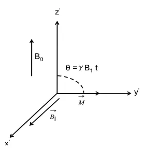
This is accomplished through the application of an RF pulse (B1 field) which rotates the magnetization into the transverse plane by an angle θ = γ B1 t (4):

Figure 2.2: Application of an RF pulse with flip angle θ = γ B1t along the x′-axis. For

(37)

For modeling any real MRI experiment, this simplified pictorial description must be

extended further to include the effects of magnetic fields produced by nuclear spins

whose Larmor frequency is different from that of water (off-resonance spins) (1, 3). The

magnetic field of these off-resonance spins, Boff, is not rotated into the transverse plane

but does result in spins experiencing an effective field (Be) which is the vector sum of Boff

and B1 (4). This concept is illustrated below:

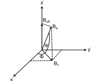
Figure 2.3: Schematic representation of the magnetic field vectors applied in the rotating frame of reference (x′, y′, z′). The B1 magnetic field is applied at an angle φ relative to the

x′-axis. Due to the presence of the magnetic field generated by off-resonance spins (Boff),

the nuclear magnetization precesses around the effective magnetic field, Be, rather than

the B1 field (1, 4, 5). The effective magnetic field is rotated away from the transverse

plane by an angle ψ.

Under the additional influence of T1 and T2 relaxation, the Bloch equation describing the

dynamics of the magnetization vector can be re-written as (6-8):

[2.7]

The first term on the right hand side of equation [2.7] accounts for the free precession of

nuclei in the external magnetic field, as well as the effects of RF and gradient pulses. The

(38)

respectively (8, 9). Equation [2.7] provides a phenomenological model of MRI spin

precession and can be used to simulate the effects of an MRI pulse sequence numerically

(10, 11). This is performed by inputting realistic values of T1, T2 and proton density and

using standard numerical methods to express equation [2.7] in matrix form as follows:

M⋅_x M⋅_y M⋅_z ⎡ ⎣ ⎢ ⎢ ⎢ ⎢ ⎢ ⎤ ⎦ ⎥ ⎥ ⎥ ⎥ ⎥ =

0 −γ G ⋅  r −γ B_1xy⋅y −γ G ⋅  r 0 γ B_1xy⋅x γ B1xy⋅y −γ B1xy⋅x 0 ⎡ ⎣ ⎢ ⎢ ⎢ ⎤ ⎦ ⎥ ⎥ ⎥ M_x M_y M_z ⎡ ⎣ ⎢ ⎢ ⎢ ⎤ ⎦ ⎥ ⎥ ⎥ +

−1/T2 0 0 0 −1/T₂ 0

0 0 −1/T₁

⎡ ⎣ ⎢ ⎢ ⎢ ⎤ ⎦ ⎥ ⎥ ⎥ M_x M_y M_z ⎡ ⎣ ⎢ ⎢ ⎢ ⎤ ⎦ ⎥ ⎥ ⎥ + 0 0 −1/T1 ⎡ ⎣ ⎢ ⎢ ⎢ ⎤ ⎦ ⎥ ⎥ ⎥ M₀ [2.8]

Equation [2.8], in discretized form, can be solved repeatedly for each repetition period in

an MRI sequence by using a numerical simulation. Understanding the time-dependent

changes in the nuclear magnetization vector plays a significant role in modeling the

changes in both the magnitude and phase signal from white and gray matter in the brain –

a major topic of discussion in this thesis.

2.2 Signal detection and Fourier domain representation of the MR imaging

experiment

After the application of the RF pulse, the nuclear magnetization will precess in the

transverse plane. The resultant time-varying magnetic field produced by the precessing

magnetization generates a current in a receiver coil located in the vicinity of the sample.

This current forms the basis for the MR image (3, 5). To more thoroughly understand this

concept, consider the Fourier relationship between the time-varying current in the coil,

s(t), and the Larmor resonance frequency, ω, of nuclei:

[2.9]

(39)

of nuclear relaxation, the Fourier relationship between the time-domain and Fourier

domain signals can be visualized as follows:

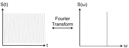
Figure 2.4: Ideal representation of the NMR signal for a sample containing pure water without T2-relaxation.

The signal in the time domain oscillates at the Larmor frequency, while the

corresponding frequency domain spectrum shows a peak at the Larmor frequency (5). In

MRI of tissues in the human body, however, multiple chemical compounds exist in a

single volume element (voxel) of the image. Each compound experiences a slightly

different local magnetic field, resulting in a modified Fourier domain representation (9)

that contains a spectrum of signals:

Figure 2.5: Representation of the NMR signal for a sample containing compounds whose protons experience different local magnetic fields (magnetic environments) without

T2-relaxation. The signal in the time domain is a composite sinusoid that oscillates at a

frequency that is the sum of the frequencies of the nuclei in different chemical

environments in the sample (3). The corresponding frequency domain spectrum displays

multiple peaks – each of which represents a specific proton in a particular magnetic

(40)

Furthermore, during any standard MRI pulse sequence, T2-based nuclear relaxation

occurs (1, 12), resulting in an exponential decay of the signal, S(t). Here the variable "t"

denotes the time after the RF pulse. The exponential decay of the signal in the time

domain corresponds to a line-broadening of the signal in the Fourier domain (1) as

illustrated below:

Figure 2.6: NMR signal for a sample of pure water subject to T2-relaxation. This results in exponential decay of the time domain signal, S(t). The line shape of the frequency

domain signal is broadened due to the exponential T2-decay process. In the simplified

representation above, the contributions of multiple resonating species with different

Larmor frequencies are neglected.

To spatially discriminate the frequency domain signal, S(ω), at one voxel from other

voxels in an image, MRI employs linear, magnetic field gradients to modulate the

amplitude of the main magnetic field (1, 12, 13). Linear modulation of the main magnetic

field (B0) enables the assignment of a unique resonance frequency to each location in the image space. The magnetic gradient field, G, is generated by a current carrying wire wound into a solenoid which produces a linear magnetic field variation along the

direction of the main field according to the following equation:

[2.10]

(41)

becoming proportional to their spatial location:

[2.11]

Through the linear relationship in equation [2.11] the desired amplitude of the gradient

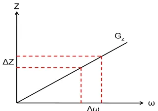
field, G, can be calculated for a particular pulse bandwidth, with Δω representing the range of frequencies excited by the RF pulse (1, 5, 13). For instance, for a gradient

amplitude of Gz and a desired slice thickness, ΔZ , the relationship between the spatial location of a slice and its Larmor frequency is depicted as follows:

Figure 2.7: Linear relationship between z-dimension slice thickness (ΔZ) of an MRI pulse sequence and the bandwidth of the RF pulse (Δω).

The MRI signal detected at a time "t" after the radiofrequency excitation pulse in

the presence of an imaging gradient is then related to the nuclear spin density by the

following Fourier relationship (12):

S(t)

=

ρ

(

→

r

−∞

∞

∫

) e

iω(r →

)t

_{d r}

→

[2.12]

where ρ(→r) represents the spin density of nuclei at a particular location. In the rotating reference frame, where the Larmor frequency is removed from the signal, equation [2.12]

(42)

S(t)= ρ(→r −∞

∞

∫ ) eiγ G r → t

d r→ _[2.13]

To express this equation in more compact form, the relationship in equation [2.13] can be

simplified (1, 5). The following change of variables is customary:

[2.14]

which, for the case of temporally-varying gradient waveforms, becomes:

[2.15]

where equation [2.15] defines the signal in the spatial frequency domain (often referred to

as k-space in MRI). The spatial frequency domain signal is related to the spin density

(ρ(r)), which is the variable of interest in MRI, through the inverse Fourier transform

operation:

[2.16]

From equation [2.16], it is clear that the relationship between the frequency domain

signal and MRI and the spatial domain spin density is through use of the inverse Fourier

transform. This relationship is represented schematically below:

(43)

The position at each point in k-space is related to the degree of image contrast variation at

a particular frequency (12). The center-most regions of k-space contain information about

the low spatial frequency components of the image. The outer-most regions of k-space

contain information about the high spatial frequency components of the image.

2.3 Gradient recalled echo imaging and T2*_contrast

Gradient recalled echo (GRE) imaging is the preferred method for acquiring complex,

T2 *

-weighted data used to isolate the image phase for LFS and QS mapping (14, 15).

GRE methods encompass a relatively large class of MRI pulse sequences that do not use

spin echoes (16). They include gradient-spoiled, RF-spoiled and balanced steady-state

free precession (bSSFP) sequences (17). A standard, gradient-spoiled GRE sequence

typically consists of an RF excitation, followed by imaging gradients and data

acquisition. The sequence is repeated many times to acquire a full imaging volume.

Figure 2.9: Pulse sequence diagram illustrating a typical gradient echo imaging sequence used in susceptibility mapping at UHF.

(44)

middle of the readout gradient. The value of TE, along with the repetition interval (TR),

flip angle and spoiling method, all influence the signal in a GRE sequence. The contrast

is also influenced by the T1, T2 and T2*

properties of the tissue (17). For example, when

the TR period is reduced below approximately 2 × T1, the spins do not regain complete longitudinal magnetization following the excitation pulse and a steady-state

magnetization is reached (14, 18). In such a steady-state, the regrowth of the longitudinal

magnetization is in equilibrium with the reduction in this magnetization caused by the RF

pulse.

If GRE imaging is preferentially sensitized to the T2*

relaxation rate (R2*

= 1/T2* ),

an image is obtained which is dominated by two parameters:(i) the rate of apparent signal

decay in an imaging voxel produced by spin-spin (R2 = 1/T2) dephasing of the transverse

magnetization (Mxy) and (ii) local magnetic field inhomogeneities (R2′ = 1/T2′) (19).

R2

*

= R2 + R2′

[2.17]

Mathematically, the influence of R2

* _{on the time-dependent MRI signal, S(t), in a GRE} experiment can be understood using the static dephasing regime theory (20). In this

regime, self-diffusion of water molecules is neglected and the MRI signal, normalized to

the voxel volume, is given by:

S(t)= 1

V ⋅ρ⋅ d  r V∫₀

⋅exp(−t⋅R₂(r  ))⋅exp(−i⋅ω( r )⋅t) _[2.18]

where ρ represents the combined effects of spin density, receiver coil sensitivity and RF

excitation efficiency. The exp(−t⋅R₂(r  )) term is proportional to the influence of R2 at a point r in the medium. The  exp(−i⋅ω(r  )⋅t) term is proportional to the influence of R2′ at a point  r in the medium and is dependent upon the geometry of the microscopic

perturbers (21). The value of the relaxation constant in a tissue can be derived from Eq.

(45)

squares fit to the resulting function:

[2.19]

where S0 represents the magnitude signal immediately after the RF pulse was applied and

t represents the time from the centre of the RF pulse to the center of the readout window.

This is schematically displayed in figure 2.10:

Figure 2.10: Schematic representation of a single repetition period for a multi-echo, GRE sequence. The α symbols denote the excitation pulses The fitted signal decay (red curve)

corresponding to equation [2.19] and corresponding measurements points (black dots) are

overlaid on the bipolar readout gradient diagram.

GRE methods are particularly useful for fast, whole brain imaging because they

employ small RF pulse flip angles and shorter repetition times compared to conventional,

spin-echo sequences. Shorter TR periods result in an overall reduced acquisition time for

volumetric imaging. Additionally, at UHF, radiofrequency heating mitigates the

amplitude of the RF pulses that can be used. The low flip angles used in GRE imaging

allows for rapid, whole-brain imaging with UHF MRI without significant tissue heating

(46)

2.4 Susceptibility imaging using gradient echo MRI at UHF

Having outlined the foundations of GRE imaging, a brief description of

electromagnetic theory applied to susceptibility processing now follows. This section

focuses on the basic physics of susceptibility contrast in MRI. A more detailed discussion

of processing and reconstruction techniques for susceptibility mapping is presented in

Chapter 3.

The human body contains a range of magnetic susceptibility values. Soft tissue

and bone are diamagnetically (negatively) shifted relative to water, with susceptibility

values ranging from 0 to -30 parts per billion (ppb) of the main magnetic field (22). In

contrast, iron and air are paramagnetically shifted relative to water, with susceptibility

values ranging from ~ 40 to 400 ppb. The exact susceptibility distribution in the brain,

however, is not known a priori (23). It is a function of tissue myelin, iron and protein

content, as well as chemical exchange and the microscopic

compartmentalization/geometry of water and lipid protons (24, 25).

To determine the susceptibility distribution in tissue, Maxwell’s equations are

used. According to the theory of magnetostatics, a given susceptibility distribution,

Δχ, produces a shift in the static magnetic field according to the Laplace equation (26):

[2.20]

The integral form of equation [2.20] can be written as:

[2.21]

where ΔB( ) denotes the magnetic field shift and θrr′ is the angle produced by the projection of the long axis of the susceptibility inclusion onto the external magnetic field

(47)

a Green’s function expansion (28). From a practical standpoint, however, numerical

computation of a solution to equation [2.21] is facilitated by transforming the integral

relationship into the Fourier domain and implementing an iterative numerical solution

(29). The resulting pointwise multiplication in the Fourier domain is given by:

F(ΔB(→r))=F(χ)×(1 3−

k_z2

k2)=F(χ)×Fd(k →

) [2.22] where F denotes the Fourier transform and Fd(k) represents the Fourier transform of the dipole convolution kernel (27). Essentially, the Fourier multiplication outlined in

equation [2.22] works by assigning a single dipole to each imaging voxel in the LFS map.

This significantly reduces the time required for the matrix inversion. However, the value

of the Fourier convolution kernel, Fd(→k) = , is not defined for k = 0 (27, 29).

The consequences of such a singularity, as well as methods for dealing with the

coefficients where k = 0, are discussed further in Chapter 3.

Chapter 2 has focused on the fundamental concepts employed in QS mapping

relevant to this thesis. Both QS mapping and the associated area of electromagnetic tissue

properties mapping constitute relatively new areas of research having the potential for

multiple future applications.

The development of a processing pipeline for multi-echo gradient-echo based

quantification of tissue magnetic properties (R2