A Study On Haar Integral and Its Methods
Amer Jasim Mohammed
Saratov State Uinversity Micanic and Mathematica, Russia
University of Baghdad, Iraq
ABSTRACT:
In this paper, an efficient numerical method for the solution of nonlinear partial
dif-ferential equations based on the Haar wavelets approach is proposed. Approximate
solutions of the generalized haar equation are compared with exact solutions. The
proposed scheme can be used in a wide class of nonlinear reaction–diffusion
equa-tions. These calculations demonstrate that the accuracy of the Haar wavelet solutions
is quite high even in the case of a small number of grid points. The present method is
a very reliable, simple, small computation costs, flexible, and convenient alternative
method. The study also compares the haar and wavelet transformation equations.
INTRODUCTION:
The past decade has witnessed
fields of science and engineering. In
and textbooks proliferating at a rapid
rate. Wavelet analysis has begun to
play a serious role in a broad range of
applications, including signal
process-ing, data and image compression,
solu-tion of partial differential equasolu-tions,
modelling multiscale phenomena, and
statistics. There seem to be no limits to
the subjects where it may have utility.
In this chapter we shall
plore some additional topics that
ex-tend the basic ideas of wavelet
analy-sis. We described the theory of wavelet
packet transforms, which sometimes
provide superior performance beyond
that provided by wavelet transforms. A
wavelet packet transform is a simple
generalization of a wavelet transform.
In this section I discussed the
defini-tion of wavelet transforms, and in the
next section examine some examples
illustrating their applications. All
wavelet packet transforms are
calcu-lated in a similar way. Therefore we
shall concentrate initially on the Haar
wavelet packet transform, which is the
easiest to describe. The Haar wavelet
packet transform is usually referred to
as the Walsh transform. [2]
Haar System:
The Haar orthogonal system begins with (t),the characteristic function of
the unit interval
(t) = x [0 , 1)(t). (1.1)
It is clear that (t) and (t - n), n 0, nZ are orthogonal since their
prod-uct is zero. It is also clear that ( t – n) is not a complete orthogonal system in
L2 (R) since its closed linear span Vo consists of 2 piecewise constant functions with
exam-In order to include more functions we consider the dilated version of (t) as
well, (2m t) where mZ. Then by a change of variable we see that 2m/2 (2m t – n)
is an orthonormal system. Vm will denote its closed linear span. Since any function in
L2 (R) may be approximated by a piecewise constant function fm with jumps at binary
rationals, it follows that is dense in L2 (R). Thus the system mn where
mn (t) = 2m/2 (2m t - n), (1.2)
is complete in L2 (R), but, since (t) and ( 2t ) are not orthogonal, it is not an
or-thogonal system. We must modify it somehow to convert it into an oror-thogonal system.
Fortunately the cure is simple; we let t 2t - 2t - 1. Then
every-thing works; t - n is orthonormal system, and 2t - k and t - n are
or-thogonal for all k and n. This enables us to deduce that mnm,nZ, where
mn (t) = 2m/2 (2mt – n), (1.3)
is a complete orthonormal system in L2 (R). this is the Haar system; the expansion of f
L2 (R)is
(1.4)
with convergence in the sense of L2 (R). the standard approximation is the series
given by
(1.5)
n m V
n mn mn m
), t ( ,
f )
t ( f
n kn kn 1
m
k
FIGURE 1: (a) The scaling function and (b) mother wavelet for the Haar system.
The Haar Transform to get that Wavelet feel
Suppose for simplicity we assume an input vector xk with 0k 7. This is
readily decomposed into an obvious basis set as shown.
1 0 0 0 0 0 0 0 0 0 0 0 0 1 0 0 0 0 0 0 0 0 1 0 0 0 0 0 0 0 0 1 7 2 10 x x x
x
xk
Other basis systems are of course possible (remember your QM and spinors?). In
1910 Haar proposed the following decomposition.
1 1 0 0 0 0 0 0 0 0 1 1 0 0 0 0 0 0 0 0 1 1 0 0 0 0 0 0 0 0 1 1 1 1 1 1 0 0 0 0 0 0 0 0 1 1 1 1 1 1 1 1 1 1 1 1 1 1 1 1 1 1 1 1 7 6 5 4 3 2 1
0 a a a a a a a
a xk
or xn Hnkak with the columns of H being simply the above basis vectors and the
a obtained by matrix inversion of H.
These basis vectors have characteristic “shapes” when drawn on their side as
shown in the figure on the next page and it is these shapes which show the
essential features of what DWT decomposition does.
Notice:
1) A mother or scaling function at the start with a non-zero average. This will
normally be normalised to 1.
2) Wavelet functions with zero average which are both compressed and
translated. It is this compression and translation which finds peaks or pulses
well.
3) The wavelet functions are orthogonal. You can see this directly by multiplying
any two together.
4) The wavelet functions have compact support which means they are all
localised. This is unlike the FT in which the basis functions
) / 2
How do we use other shapes and make a wavelet basis system out of them?
step 1: Mother functions
Let (x)be some mother function. The (2x) is the same function compressed by a
factor of 2. Binary compression can therefore be denoted as j (2jx). Likewise
) 1 2 ( x
is our compressed function translated by 1. Multiple translation and
compression of the mother function can therefore be denoted as jk (2jxk)
We do not choose (x) arbitrarily but impose two conditions.
1)
k
k x k
c
x) (2 )
(
or more generally
k
j j k j
k x c
x) (2 )
2
( 1
. That is it
lends itself to a fractal like summing behaviour.
2)
(x)dx1, the normalisation condition. This leads to
2k k
c . Alas, life is not
then you will NOT get coefficients which produce a reversible transform. Since this is
desirable in physics we need to do what Numerical Recipes suggests and force
1
2
k k
c . This means reducing the coefficients by a further factor 2
1 . The reason
lies buried deep in matrix inversion.
Here are two examples, our friend Haar and the “top hat”
Again a 1 2 multiplication factor ensures reversibility of the transform
Ingrid Daubechies invented a four coefficient fractal which is not a simple mother
function shape as above, but instead must be constructed by working backwards
from the coefficients. They are:
) 3 1 ( 4 1 ), 3 3 ( 4 1 ), 3 3 ( 4 1 ), 3 1 ( 4 1
3 2
1
0 c c c
c
Again “Numerical Recipes” surreptitiously adds a further 1 2 and with good
step2: Wavelet functions
From the mother or scaling function and the coefficients we construct
wave-let functions (x).
) 2 ( )
1 ( )
(x cM k x k
k k
or at other compression levels
) 2 ( )
1 ( ) 2
( 1x cM k jx k
k k j
with generally
) 2 ( )
1
( c jx k
k M k
k
jk
Three things to note:
1) The introduction of an alternating negative sign on the coefficients.
2) The inversion of the order of coefficients assuming there are M coefficients.
3) If you have multiplied by the requisite fudge factor to get a reversible
transform you don’t need to do any more on these coefficients.
Here are the basic wavelet shapes at the highest level. The Daubechies wavelet is
Please note the wavelet function for the top hat is strictly
) 2 2 ( 2 1 ) 1 2 ( ) 2 ( 2 1 )
(x x x x
and inverted to the above diagram. The areas
sum to zero as does the sum of the coefficients.
step3: Multi Resolution Analysis (MRA)
Although we have quite general definitions for jk and jk we need only use the
j=0 level over and over again. This was a discovery by Mallet.
Here is the technique:
2 4 2 6 3 5 1 5 1 3 2 4 1 4 2 3 1 1 1 1 w m w m w m w m
2) Now sort (an effective permutation) the above column matrix and bring all the
mother generated coefficients to the top.
2 2 3 1 4 6 5 5 2 4 4 6 3 5 1 5 w w w w m m m m
3) Now repeat step 2 only on the coefficients labelled ‘m’
2 2 3 1 2 10 0 10 2 2 3 1 4 6 5 5 1 1 1 1
4) repeat step 2) and 3) until only the top coefficient has the ‘m’ label.
2 2 3 1 2 0 0 20 2 2 3 1 2 0 10 10 2 2 3 1 2 10 0 10 2 2 3 1 4 6 5 5 2 4 2 6 3 5 1 5 1 3 2 4 1 4 2 3 T P T P T
Reversing the above procedure is used to compose the original vector. In this case
the multiplying matrix has to be.
12 2 1 2 1 2 1
which is the inverse of the original coefficient matrix. But this is messy and could
be fixed with a universal 1/ 2 to retain the symmetry of the mathematics and is
why “Numerical Recipes” adds the factor to the coefficients.
Check for yourself reverse sequence is:
1 3 2 4 1 4 2 3 2 4 2 6 3 5 1 5 2 2 3 1 4 6 5 5 2 2 3 1 2 10 0 10 2 2 3 1 2 0 10 10 2 2 3 1 2 0 0 20 T P T P T
The reverse procedure is created by multiplying pairs by the transpose of the
original matrix of coefficients as shown. This also effectively changes the order of
the coefficients.
One of the intrinsic advantages of the wavelet transform is that only requires an
order(N) computational effort and is much faster than the FFT at vector
transformation..
Walsh Function:
The Rademacher functions are an orthogonal system on (0, 1) obtained by
adding up all the Haar functions at the same scale. The Rademacher functions were
obtained by combining the Haar functions by simply adding them at a given scale.
The Walsh functions take sums and differences of the Haar functions to obtain a
com-plete system. We define
Wo (t) : = (t), w1 (t) : = (t),
W3 (t) : = (2t) - (2t - 1),
W2n (t) : = Wn (2t) + Wn (2t - 1),
W2n+1 (t) : = Wn (2t) - Wn (2t - 1).
(1.6)
Thus these Walsh functions also belong to the wavelet subspaces of the Haar system:
W0 V0 , W1 W0, W2 , W3 W1 , W4 , W5 , W6, W7 W2 ,...
W2m, W2m+1,..., W2m+1-1 Wm,...
(1.7)
Notice that these defining relations (1.7) are exactly the same as those in the
two dilation equations of the Haar system,
(t) = (2t) + (2t – 1), (1. 8a)
(t) = (2t) - (2t - 1). (1. 8b)
Since all functions defined by (1.8a) are orthogonal to all defined by (1.8b),
it follows that W2n and W2n+1 are orthogonal. Also if Wn and Wm are orthogonal so are
W2m, W2m+1, …, W2m+1-1 are orthogonal in Wn. Since all of these functions have
sup-port contained in [0,1], the {Wn} are an orthogonal system in L2 (0,1). Moreover,
there are exactly 2m Haar functions in Wm whose support lies in [0,1], and therefore
the Walsh functions in Wm form a basis of this space. Since the Haar functions are
FIGURE 2 One of the Rademacher functions
Comparing Haar Transform with Walsh Transform:
The Haar wavelet packet transform is usually referred to as the Walsh
trans-form. A Walsh transform is calculated by performing a 1-level Haar transform on all
subsignals, both trends and fluctuations.
For example, consider the signal f defined by
f = (4, 6, 8, 10, 12, 14, 16, 18). (1.9)
A 1-level Haar transform:
(1.10)
A 1-level Haar transform and a 1-level Walsh transform of f are identical,
producing the following signal:
(1.11)
A 2-level Walsh transform is calculated by performing 1-level Haar
trans-forms on both the trend and the fluctuation sub signals, as follows:
. 2
18 16 , 2
14 12 , 2
10 8 , 2
6 4 2
18 16 , 2
14 12 , 2
10 8 , 2
6 4
5 2,9 2,13 2,17 2 2, 2, 2, 2
.Amplitude
Time
1
1
(1.12)
Hence the 2-level Walsh transform of the signal f is the following signal:
(14, 30 | -4, -4 | -2, -2 | 0, 0). (1.13)
It is interesting to compare this 2-level Walsh transform with the 2-level
Haar transform of the signal f. The 2-level Haar transform of f is the following signal
:
(1.14)
comparing this Haar transform with the Walsh transform in (1.13), we see that the
Walsh transform is slightly more compressed in terms of energy, since the last two
values of the Walsh transform are zeros. We could, for example, achieve 25 %
com-pression of signal f by discarding the two zeros from its 2-level Walsh transform, but
we could not discard any zeros from its 2-level Haar transform. Another advantage of
the 2-level Walsh transform is that it is more likely that all of its non-zero values
would stand out form a random noise background, because these values have larger
magnitudes than the values of the 2-level Haar transform.
A 3-level Walsh transform is performed by calculating 1-level Haar
trans-forms on each of the four sub signals that make up the 2-level Walsh transform. For
example, applying 1-level Haar transforms to each of the four sub signals of the
2-level Walsh transform, we obtain
.2 2 2
, 2
2 2
, 2
2 2 , 2
2 2 2
, 2 , 2 ,
2
14,30 4,4 2, 2, 2, 2
,), 2 8 2 22 ( ) 30 , 14
(1.16)
Here, at the third level, the contrast between the Haar and Walsh transforms
is even shaper than at the second level. The 3-level Haar transform of this signal is
(1.17)
comparing the transforms (1.16) and (1.17) we can see, at least for this particular
sig-nal f, that the 3-level Walsh transform achieves a more compact redistribution of the
energy of the signal than the Haar transform.
APPLICATIONS OF HAAR TRANSFORMS
In this section we shall discuss two examples of applying wavelet packet
transforms to audio and image compression. While wavelet packet transforms can be
used for other purposes, such as noise removal, because of space limitations we shall
limit our discussion to the arena of compression.
First example, we shall use a Coif 30 wavelet packet transform to compress
the audio signal greasy. If we found that a 4-level Coif 30 wavelet transform – with
trend values quantized at 8 bpp and fluctuations quantized at 6 bpp, and with separate
entropies computed for all sub signals achieved a compression of greasy requiring an
estimated 11,305 bits. That is, this compression required an estimated 0.69 bpp
(in-stead of 8 bpp in the original). However, if we use a 4-level Coif 18 wavelet packet
transform and quantize in the same way, then the estimated number of bits is 10.158
i.e, 0,62 bpp. This represents a slight improvement over the wavelet transform.
In several respects – in bpp, in RMS Error, and in total number of –
signifi-cant values – the wavelet packet compression of greasy is nearly as good as or slightly
better than the wavelet transform compression. See Table1.1
), 2 , 2 , 2 , 2 4 , 4 2 8 2 22
Transform Sign.Values Bpp RMS Error
wavelet 3685 0.69 0.839
w.packet 3072 0.62 0.868
TABLE 1.1 Wavelet and wavelet packet compressions of greasy
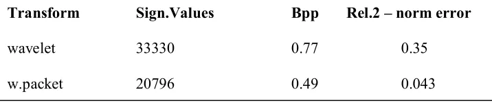
Second example, we consider a compression of a fingerprint image. Using
the quantizations 9bpp for the trend and 6bpp fort the fluctuations, we obtain an
esti-mated 0.49bpp. That represents a 36 % improvement over the 0,77bpp estiesti-mated for
the wavelet compression. In Table 1.2 I show a comparison of these two
compres-sions of Fingerprint 1. Although the wavelet packet transform compression does not
produce as small a relative 2-norm error as the wavelet transform compression,
never-theless, a value of 0.043 is still better than the 0.05 rule of thumb value for an
accept-able approximation. Taking into account the other data from Table 1.2 – the number
of significant transform values and the number of bpps – it is clear that the wavelet
packet compression of Fingerprint 1 is superior to the wavelet compression. [2]
Transform Sign.Values Bpp Rel.2 – norm error
wavelet 33330 0.77 0.35
w.packet 20796 0.49 0.043
TABLE 2: Two compressions of Fingerprint 1
CONTINUOUS WAVELET TRANSFORM
translating (displacing) it. The word continuous refers to transform, not the wavelets,
although people sometimes speak of “continuous wavelets”.
The continuous wavelet transform turns a signal f (t) into a function with two
variables (scale and time), which one can call c (a,b) :
(2.1)
This transformation is in theory infinitely redundant, but it can be useful in
recognizing certain characteristics of o signal. In addition, the extreme redundancy is
less of a problem than one might imagine, a number of researchers have found ways
of rapidly extracting the essential information from these redundant transforms.
One such method reduces a redundant transform to its skeleton. When certain
signals are represented by a continuous wavelet transform, all the significant
informa-tion of the signal is contained in curves, or “ridges” says Bruno Torréssani of the
French Centre National de Recherché Scientifique, who works at the University of
Aix – Marseille II. These are essentially the points in the time – frequency plane
where the natural frequency of the translated and dilated wavelet coincides with the
local frequencies, or one of the local frequencies, of the transform. [3]
Haar wavelet is the simplest wavelet. The Haar wavelet transform, proposed in 1909
by Alfred Haar, is the first known wavelet. Haar transform or Haar wavelet transform
has been used as an earliest example for orthonormal wavelet transform with compact
support. The Haar wavelet family for x ϵ [0, 1] is defined as follows:
. dt ) b at ( ) t ( f ) b , a (
where and . In these formulae integer m = 2j, j = 0, 1, … J
indicates the level of the wavelet; k = 0, 1, … m − 1 is the translation parameter.
Max-imal level of resolution is J and 2J is denoted as M = 2J. The index i is calculated from
the formula i = m + k + 1; in the case of minimal values m = 1, k = 0 we have i = 2.
The maximal value of i is i = 2M = 2J+1. It is assumed that the value i = 1 corresponds
to the scaling function for which h1(x) = 1.
It must be noticed that all the Haar wavelets are orthogonal to each other:
Therefore, they construct a very good transform basis. Any function y(x), which is
square integrable in the interval [0, 1), namely is finite, can be expanded in
a Haar series with an infinite number of terms
Where the Haar coefficients,
are determined in such a way that the integral square error
In general, the series expansion of y(x) contains infinite terms. If y(x) is a piecewise
constant or may be approximated as a piecewise constant during each subinterval,
then y(x) will be terminated at finite terms, that is
where the coefficient and the Haar function vectors are defined as:
respectively and x∈[0,1)x∈[0,1).
The integrals of Haar function hi(x) can be evaluated as:
pi,1(x)=∫0xhi(x)dx
Carrying out these integrations with the aid, it is found that
Let us define the collocation points xl = (l − 0.5)/(2M), l = 1, 2, …, 2M. By these
col-location points, a discretizised form of the Haar function hi(x) can be obtained. Hence,
the coefficient matrix H(i, l) = (hi(xl)), which has the dimension 2M × 2M, is
achieved. The operational matrices of integrations Pυ, which are 2M square matrices,
are defined by the equation Pυ(i, l) = pi,υ(xl), where υ shows the order of integration.
CONCLUSION:
In this paper, Haar equation is
pro-posed for the generalized wavelet
transformation equation. Comparisons
of the haar and wavelet transformation
show that our method is efficient
method. These calculations
demon-strate that the accuracy of the Haar
wavelet solutions is quite high even in
the case of a small number of grid
tions of the problems. These are the
main advantages of the method. Hence,
the present method is a very reliable,
simple, fast, minimal computation
costs, flexible, and convenient
alterna-tive method.
REFERENCES
Walter, Gilbert G. & Shen,
Xiaop-ing, Wavelets and Other
Walker, J.S., A Primer on Wavelets
and Their Scientific Applications,
Printice-Hall Inc., 1999.
Resnikoff, Howard L. & Wells,
Raymond O., Wavelet Analysis,
Springer-Verlag New York Inc.,
1998.
Hubband, Barbara Burke, The
World According to Wavelets,
AK Peters Ltd., 1995.
Vetterli, Martin & Kovacevic,
Jelena, Wavelets and Subband
Coding, Printice Hall Inc., 1995.
Benedetto, John J. & Frazier,
Micheal W., Wavelets :
Mathe-matics and Applications, CRC
Press Inc., 1994.
7. Daubechies, Ingrid, Ten
Lec-tures on Wavelets, Capital City
Press, 1992.
Bredon, Glen E. "A new treatment
of the Haar integral." The
Michi-gan Mathematical Journal 10.4
Dubins, Lester E. "Measurable tail
disintegrations of the Haar
integral are purely finitely
addi-tive." Proceedings of the
Ameri-can Mathematical Society 62, no.
1 (1977): 34-36.
Williams, David, and John F.
Cornwell. "The Haar integral for
Lie supergroups." Journal of
ma-thematical physics 25, no. 10