Demand Response based Unit Commitment
Manisha Govardhan
Research Scholar, Dept. of Electrical Engineering, S.V. National Institute of Technology, Surat, Gujarat, India
ABSTRACT: The predominant power system problem of energy crisis is mainly due to growing load demand and non-renewability of the traditional energies. Demand response program (DRP) is an influencing load shaping tool against continuous change in load demand due to the intermittent and the volatile nature of the renewable energy sources (RES) integrated into the modern power system. In DRP, customer behaviour is mainly influenced by the different incentive values offered and variations in price elasticity matrix elements. In this paper, the demand response based unit commitment problem (DRUCP) has been considered to investigate the customers’ behaviour under different case studies of varying incentive values and price elasticity matrix elements and their associated change in load demand and total cost of the system. The simulation study is carried out using Global best Artificial Bee Colony (GABC) algorithm for a microgrid system considering solar and wind renewable sources. It is found that implementation of DRP significantly reduces the total cost of the system.
KEYWORDS:Demand Response Program (DRP), Global best Artificial Bee Colony (GABC) Algorithm, Price Elasticity Matrix (PEM), Renewable Energy Sources (RES), UnitCommitment Problem (UCP).
I.INTRODUCTION
Growing energy demand and limited generation resources require an enhanced power system with appropriate demand side management with customer based demand response program (DRP). DRP is an organized approach to reduce the load demand againsta rise in electricity price during peak hours of the day and thereby reshaping the load curve. The financial benefit is a chief motive for the customers participating in the DRP and hence, customers tend to maximize their benefit by reducing their electricity usage with the change in electricity price during the day. According to Federal Energy Regulatory Commission (FERC), demand response can be defined as the changes in electricity usage by the end user entities from their normal energy consumption patterns in response to the changes in the price of electricity or to incentive payments designed to induce lower electricity use at times of high wholesale market prices or when system reliability is jeopardized [1].
FERC has classified different DRPs into two main categories, namely, incentive based programs (IBP) and time based programs (TBP). The extensive IBP offers cash or discount in bill to the customers for reducing their electricity consumption during peak hours or during periods of high electricity price [2]. This IBP is broadly classified into [1]: Demand bidding/buyback (DB) program, direct load control (DLC), emergency demand response program (EDRP), interruptible load program, load as capacity resource, non-spinning reserves, regulation services and spinning reserves programs [1]. The well-known TBP motivates the customers to shift their load from peak hours to low load or off- peak hours and reshape the inconsistent load demand curve. The TBP mainly comprises: Critical peak pricing with control, peak time rebate, real-time pricing, time-of-use pricing and system peak response transmission tariff [1]. However, with demand side management, appropriate generation scheduling is a crucial optimization problem with two sub problems of power system, namely, unit commitment problem (UCP) and economic load dispatch (ELD). UCP deals with the on/off status judgment of the generating units over a scheduled period and ELD dispenses generated power among the committed units while satisfying multiple constraints to obtain minimum generation cost.
discussion of demand-side resources (DSRs) with different linear and non-linear models of responsive loads linked with supply-side resources (SSRs) to solve UCP is given in [7]. The commercial concept of DRPs with UCP is solved in [8] and day-ahead scheduling model with hourly DRP considering ramping cost of generating unit is discussed in [9]. In [10], authors have discussed customer sensitivity towards different values of incentive and penalty offered to them for several cases of price elasticity matrix elements under demand response program.
The main objective of this study is toinvestigatethe impact of DRP on UCP and to study the customers’behaviourfor different incentive values and variation in price elasticity matrix (PEM) elements. The simulation study is carried out by employing an efficient Global best artificial bee colony (GABC) optimization algorithm. The deployment of the rest of this paper is as follows: Section 2 describes the load economic model of the DRP. Formulation of DRUCP model including solar and wind renewable sources is presented in section 3. A brief review of the GABC optimization algorithm is given in section 4. Section 5 deliberates the simulation results and comparisons of different cases considered. The conclusion is drawn in section 6.
II.DEMAND RESPONSE MODELLING STRUCTURE
In deregulated electricity market, customer participation can be accessed from the economic model of load demand which reveals the change in load demand with the change in the price of electricity and incentives offered to them during several periods of the day. This demand elasticity (E) pertaining to price is defined as [11]:
o L
Lo
EP P
E
P EP
(1)
According to (1), price elasticity of the hth time with respect to jth period can be written as [11]:
( ) ( ) ( , )
( ) ( )
o j L h h j
Lo h j
EP P
E
P EP
(2)
whereEPo and EP are the electricity price before and after implementation of the DRP. Likewise, PLoand PL are the load
demand before and after implementing DRP.
EP
and
P
L describe the change in electricity price and load demand from their initial values respectively.Customer behavior is characterized according to the load variation with respect to electricity price. There are certain stiff loads which cannot shift from one period to another period with the price variation and sensitive to single period only termed as self-elasticity. Furthermore, some flexible loads can vary from peak hours to low load periods having sensitivity to multi-period can be defined as cross elasticity. Hence, customer behavior for 24 hours can be symbolized by price elasticity matrix (PEM) which is a 24×24 matrix with self-elasticity coefficients as diagonal elements and cross elasticity coefficients as off-diagonal elements [11].A) Single period loads
In DRP,the participating customers change their load demand according to the incentive value (A) offered to them. An incentive paid to the customer in hthhour for reduction of each kWh load demand is given as [11]:
( ) ( )[ ( ) ( )]
DR h h Lo h L h
C A P P
(3) The total benefit of the participating customer in hth hour can be written as [11]:
( ) ( ) ( ) ( )
( ) * ( )
B L h L h h L h
T B P P EP A P
(4)
Total maximum benefit can be attained by making TB PL h( ) 0 which results in:
( )
( ) ( ) ( )
( )
( )
L h
h h
L h B P
EP A
P
(5)
( ) ( ) ( ) ( ) ( ) ( ) ( )
( ) ( )
( L h ) o h o h[ L h Lo h ] 1 L h Lo h h Lo h
P P
B P B EP P P
E P
(6)
After differentiating (6) with respect to PL(h) and substituting the result into (5), the expression obtained is:
( ) ( ) ( ) ( ) ( )
( ) ( )
1 L h Lo h
h h o h
h Lo h
P P
EP A EP
E P
(7)
Hence, participating customer’s consumption will be described as:
( ) ( ) ( ) ( ) ( ) ( , )
( )
1 h o h h
L h Lo h h h
o h
EP EP A
P P E
EP (8)
B) Multi-period loads
Assuming price elasticity as a constant value that is [12]:
( ) ( ) L h j P EP
Constant for h, where j=1, 2……..24.
(9)
By relating prices and demands linearly, multi-period load model obtained is:
( ) ( ) ( ) ( ) ( ) ( , ) ( ) 1 1 T
j o j j
L h Lo h h j
o j j
j h
EP EP A
P P E
EP
(10)C) Load economic model
The combination of (8) and (10) results in load economic model as follows [11]:
( ) ( ) ( ) ( ) ( ) ( ) ( ) ( ) ( , ) ( , )
( ) 1 ( )
1
T
h o h h j o j j
L h Lo h h h h j
o h j o j
j h
EP EP A EP EP A
P P E E
EP EP
(11)Assuming an equal value of electricity price before and after implementation of DRP (i.e. EPo = EP) and βas possible
customer participation (in %) in the DRP, equation (11) can be written as:
( ) ( ) ( ) ( ) ( , )
( ) 1
(1 ) 1
T
j
L h Lo h Lo h h j
o j j
A
P P P E
EP
(12) III.PROBLEM FORMULATIONThe classic UCP performs optimal scheduling of generating units after appropriate on/off decision of generating units to attain minimum generation cost while handling load demand, power balance, spinning reserve, generation limits and minimum up/down constraints over a scheduled period of 24 hours. Furthermore, initial status (IS) of each generating unit must consider before commencement of scheduling. The objective function of DRUCPmodel characterized as:
( ) ( ) ( ) ( ) ( )( 1) ( ) 1 1
min (1 )
N T
i h i h i h i h i h DR h i h
TC FC u SUC u u C
(13)where FCi(h) and SUCi(h) are referred to as the fuel cost and start-up cost of ith thermal unit at hour h respectively. TC
participation in the DRP at hour h.Furthermore, N and T represent the total number of generating units and scheduled time period respectively. The thermal unit index and hour index are symbolized asi and h respectively and u indicates the on /off status of the thermal units (1= on and 0 = off). The fuel cost of generating unit in quadratic polynomial function of power generated is classically expressed as:
2 ( ) ( ) ( )
i h i i gi h i gi h
FC a b P c P (14)
whereai, bi and ci are the fuel cost coefficients of each thermal unit iand Pgi(h) refers as power generated from unit i at
hour h. The start-up cost is categorized as hot start-up cost (h_cost) and cold start-up cost (c_cost) depending on the temperature of a thermal unit and can be given as:
( ) ( ) ( ) ( )
( ) ( )
_ cos
_ cos
off
i h i h i i h i
i h off
i h i i h i
h t if MD T MD CSH
SUC
c t if T MD CSH
(15)
whereMD, Tioff and CSH are denoted as minimum down time, minimum off time and cold start hour respectively. The
execution of the above DRUCP model must satisfy several constraints listed below:
Power balance constraint: The accumulation wind power (PW), solar power (PS) along with the generated power from
the thermal units must satisfy the load demand as [13]:
( ) ( ) ( ) ( )
gi h W h S h L h
P P P P (16)
The generated output power from the wind turbine model is calculated as [14]:
3 ( )
( )
0
h R
W h R
q v z P
P P
( )
( )
ci h r r h co
v v v
v v v
otherwise
(17)
whereqPR/ (vr3vci3) and zvci3/ (vr3vci3). Also, vc, vco ,vrand PR are referred to as cut-in, cut-out, rated
speed and rated power output of wind turbine respectively.
The power output of photovoltaic module depends on area ( ) and efficiency of pv model () and solar radiation (G) is calculated as [15]:
( ) ( )
S h h
P G (18)
Generation limit constraint: Power output of each generating unit must be within its minimum (Pgmin) and maximum
(Pgmax) limits as:
min max
gi gi gi
P P P (19)
Spinning reserve constraint: Usually, a certain amount of spinning reserve (SR) has to be maintained for system reliability as:
max
( ) ( ) ( ) 1
N
gi i h Lnew h h i
P u P SR
Minimum up/down constraint: Each thermal unit must remain on/off for the particular time duration before any transition occurs.
on
i i
off
i i
T MU
T MD
(21)
whereTion and MU are the minimum on time and minimum up time respectively.
IV.OVERVIEW OF GABC ALGORITHM
Karaboga has developed the basic concept of artificial bee colony algorithm which emphases the food finding habits of honeybees. The artificial bees are mainly distributed into three groups, namely, employed bees, onlookers and scouts [16]. These bees fly in multidimensional search space to pursue their food source. Employed bees use their own experience to find the food source while scout bees hunt their food source arbitrarily. The onlooker bees pick good food source from those founded by the employed bees and they further search food source nearby the selected food source. Each food source signifies the possible solution of the optimization problem and quality of the food source is judged by the nectar amount of the food source. In ABC,the initial population P of Np possible solution is generated randomly.
Each Pi (i= 1, 2,……Np) is a D dimensional vector where D is the number of optimized parameters. In employed bee
phase, the new random food source is generated as follows:
( )
i j i j i j ij kj
v P P P (22)
wherePij andvij indicate the previous and new food source respectively andijdenotes a random number between 0 to
1, j € {1,2…D} and Pk indicates an alternative solution chosen randomly from the population. In GABC, global best
(gbest) solution is used to improve the search mechanism and the equation (22) is modified as [17]:
( ) ( )
i j i j i j ij kj ij j i j
v P P P y P (23)
The added term in (23) is gbest term, yj is the jth element of the global best solution and Ψij is a random number in [0, C] where C is a nonnegative constant. In onlooker phase, each onlooker bee chooses a food source according to the probability value pi = fiti/ Σnfitn wherefit describes the fitness of a solution. Thereafter, onlooker bees further searches
for better solution (food source) in the neighbourhood of the selected one according to (23). If the solution has not improved after certain trials, then scout bees generate new food source and repeat the hunting process.
V. RESULT AND DISCUSSION
Table 1 Microgrid system data
Unit Pgmax
(kW)
Pgmin
(kW)
a
(cts/h)
b
(cts/kWh)
c
(cts/kWh2)
MU
(h)
MD
(h)
h_cost
(cts)
c_cost
(cts)
CSH
(h)
IS
(h)
1 410 100 65 15.20 0.00052 5 5 550 1100 3 5
2 410 100 60 15.30 0.00061 5 5 500 1000 3 5
3 270 50 45 16.60 0.00210 3 3 450 900 2 3
4 270 50 41 16.50 0.00211 3 3 460 920 2 3
5 140 25 40 18.50 0.00420 2 2 800 1600 1 2
6 140 25 38 18.76 0.00530 2 2 750 1500 1 -2
7 90 20 38 26.70 0.00080 2 2 360 720 1 -2
8 90 20 35 26.90 0.00120 2 2 350 700 1 -2
9 65 15 30 29.71 0.00090 1 1 280 560 0 -1
10 65 15 24 29.92 0.00130 1 1 285 570 0 -1
11 45 10 18 26.20 0.00240 1 1 200 400 0 -1
12 45 10 15 26.79 0.00310 1 1 205 410 0 -1
Table 2 Solar and wind parameters
PV system (1×360kWp) Wind Plant (3×140kWp)
1659×870 mm PR=140 kW vci=3 m/sec
15 % vr=12 m/sec vco=25 m/sec
Table 3 Hourly load demand and market price
Hour 1 2 3 4 5 6 7 8 9 10 11 12
Demand (kW) 1000 1030 1050 1070 1090 1150 1300 1400 1640 1700 1870 1870 EP(cts) 29.8 29.9 30.0 30.1 30.2 30.3 30.4 30.5 30.6 30.7 30.8 30.9
Hour 13 14 15 16 17 18 19 20 21 22 23 24
Demand (kW) 1850 1800 1720 1700 1650 1630 1550 1450 1350 1200 1150 1050 EP(cts) 30.9 30.8 30.7 30.6 30.5 30.4 30.3 30.2 30.1 30.0 29.9 29.8
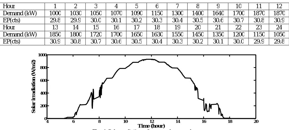
Fig. 1 Solar radiation of a normal sunny day
4 6 8 10 12 14 16 18 20
0 200 400 600 800 1000
Time (hour)
S
o
la
r
ir
ra
d
ia
ti
o
n
(
W
/m
2
Fig. 2 Wind speed of a normal day
Table 4 Price elasticity matrix
Low Off-peak Peak Off-peak
Low -0.04 0.05 0.04 0.05
Off-peak 0.05 -0.16 0.02 0.04
Peak 0.04 0.02 -0.16 0.02
Off-peak 0.05 0.04 0.02 -0.16
Table 5 Different cases
cases Incentive offered Price elasticity matrix
1 - -
2 4 As Table.4
3 8 As Table.4
4 2 As Table.4
5 4 As double the value of Table.4
6 4 As half the value of Table.4
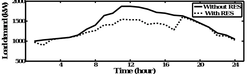
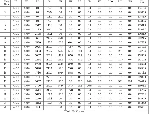
Case 1: UCP is solved considering the effect of RES without implementing DRP in this case. This case is assumed as the base case for the rest of the study. The generation scheduling with total generation cost using GABC is presented in Table.6. From Table.6, it can be seen that the generating units U1 to U4 share major portion of the load demand and the other units U5 to U12 are committed to satisfy the power balance and spinning reserve constraints. Integration of wind and solar RES with thermal units reduces the load demand, whichresults in a total cost of516643.2 cents. Plot of load demand without and with RES is shown in Fig.3 which yields that the availability of renewable energy significantly reduces the overall load demand and hence, the total cost of the system
Fig.3 Load demand with and without RES
1 2 4 6 8 10 12 14 16 18 20 22
0 5 10 15
Time (hour)
W
in
d
s
p
ee
d
(
m
/s
ec
)
4 8 12 16 20 24
500 1000 1500 2000
Time (hour)
L
o
a
d
d
em
a
n
d
(
k
W
)
Case 2, 3, 4: These cases are solved to investigate the customers’ behavior for varying incentive values. The incentive values considered are 4 cents (as base), 8 cents (double of base) and 2 cents (as half of base) for case 2, case 3 and case 4 respectively. For case 2, the generation cost obtained is 506975.2 cents which result in 1.43 % reduction in the total cost as compared to the case 1. In case 3, load demand is reduced and in case 4, load demand is raised compared to case 3 which indicates that customers’ concern is highly inclined towards the offered incentive value. The total amount of incentive paid to the customers are 2274.6 cents, 9098.0 cents and 568.62 cents in cases 2, 3 and 4respectively, which indicate that the customers tend to participate more actively in the DRP as incentive value increases. As the customer benefit rises, net utility profit and % reduction in cost decays and vice a versa. The load demand plots of these three cases are shown in Fig.4.
Table 6 Optimul generation scheduling
Unit/ Hour
U1 U2 U3 U4 U5 U6 U7 U8 U9 U10 U11 U12 TC
1 410.0 410.0 0.0 152.0 0.0 0.0 0.0 0.0 0.0 0.0 0.0 0.0 15418.4
2 410.0 410.0 0.0 79.5 0.0 0.0 0.0 0.0 0.0 0.0 0.0 0.0 14186.5
3 410.0 410.0 0.0 101.0 115.0 0.0 0.0 0.0 0.0 0.0 0.0 0.0 17572.5
4 410.0 410.0 0.0 162.3 87.7 0.0 0.0 0.0 0.0 0.0 0.0 0.0 17289.6
5 410.0 410.0 154.2 115.8 0.0 0.0 0.0 0.0 0.0 0.0 0.0 0.0 17904.6
6 410.0 410.0 227.3 85.2 0.0 0.0 0.0 0.0 0.0 0.0 0.0 0.0 18209.7
7 410.0 410.0 210.5 187.1 0.0 0.0 0.0 0.0 0.0 0.0 0.0 0.0 19654.9
8 410.0 410.0 169.1 249.2 25.0 0.0 0.0 0.0 0.0 0.0 0.0 0.0 21321.5
9 410.0 410.0 256.9 145.5 120.6 60.4 0.0 0.0 0.0 0.0 0.0 0.0 24776.5
10 410.0 410.0 202.5 270.0 77.7 42.7 0.0 0.0 0.0 0.0 0.0 0.0 23313.4
11 410.0 410.0 238.3 262.7 54.4 123.0 21.1 0.0 0.0 0.0 26.1 0.0 27373.4
12 410.0 410.0 206.7 268.2 112.9 87.0 38.2 0.0 0.0 0.0 0.0 0.0 25956.5
13 410.0 410.0 223.4 270.0 138.3 31.4 30.2 0.0 0.0 0.0 19.7 0.0 26219.2
14 410.0 410.0 270.0 267.4 25.0 37.9 0.0 0.0 0.0 0.0 0.0 0.0 23365.8
15 410.0 410.0 269.0 210.4 127.0 25.0 0.0 0.0 0.0 0.0 0.0 0.0 24056.5
16 410.0 410.0 174.6 270.0 89.9 55.8 0.0 0.0 0.0 0.0 0.0 0.0 23314.2
17 410.0 410.0 88.1 270.0 102.9 0.0 0.0 0.0 0.0 0.0 0.0 0.0 20982.0
18 410.0 410.0 268.7 270.0 140.0 0.0 20.0 20.0 0.0 0.0 39.1 28.7 30047.3
19 410.0 410.0 270.0 270.0 57.9 37.3 56.2 20.6 0.0 0.0 0.0 0.0 26904.2
20 410.0 410.0 254.4 218.2 72.4 76.8 0.0 0.0 0.0 0.0 0.0 0.0 23878.5
21 410.0 410.0 269.3 137.4 123.3 0.0 0.0 0.0 0.0 0.0 0.0 0.0 22220.4
22 410.0 410.0 129.0 184.1 0.0 0.0 0.0 0.0 0.0 0.0 0.0 0.0 18190.5
23 410.0 410.0 181.3 127.8 0.0 0.0 0.0 0.0 0.0 0.0 0.0 0.0 18126.9
24 410.0 410.0 97.4 108.6 0.0 0.0 0.0 0.0 0.0 0.0 0.0 0.0 16360.1
Fig. 4 Load demand variation for different incentive values
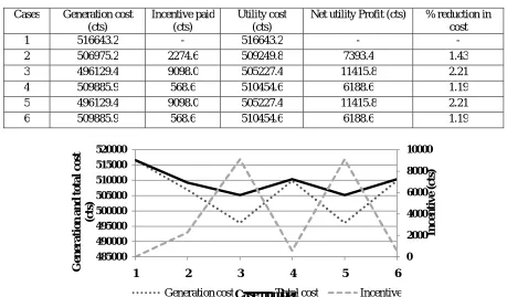
Case 5, 6:These cases are considered to comprehend the effect of varying price elasticity matrix (PEM) elements with base incentive. In case 5, PEM elements are doubled and in case 6 PEM elements are divided by 2 which result in duplication of case 3 and case 4 respectively. These two cases reveal the fact that PEM is a measure of customer participation in the DRP. The higher PEM elements specify more customer flexibility towards load shifting with higher benefit while lower PEM elements indicates that the customers become stiff and less sensitive to load shifting causing minimum benefit.The summarized results table for all cases is given in Table.6.The comparison of different costs for different cases is given in Fig. 5 which shows that minimum generation cost and utility costs are achieved in case 3 and case 5 due to higher incentive value and price elasticity matrix elements with a maximum incentive offered to the customers.
Table 6 Cost comparison of different cases
Cases Generation cost (cts)
Incentive paid (cts)
Utility cost (cts)
Net utility Profit (cts) % reduction in cost
1 516643.2 - 516643.2 - -
2 506975.2 2274.6 509249.8 7393.4 1.43
3 496129.4 9098.0 505227.4 11415.8 2.21
4 509885.9 568.6 510454.6 6188.6 1.19
5 496129.4 9098.0 505227.4 11415.8 2.21
6 509885.9 568.6 510454.6 6188.6 1.19
Fig .5Comparisons of different costs for different cases
0 5 10 15 20 25
800 1000 1200 1400 1600
Time (hour)
L
o
a
d
d
em
a
n
d
(
k
W
)
Half insc. Base insc. Double insc.0 2000 4000 6000 8000 10000
485000 490000 495000 500000 505000 510000 515000 520000
1 2 3 4 5 6
In
c
e
n
ti
v
e
(c
ts
)
G
e
n
e
r
ati
o
n
an
d
to
tal
c
o
st
(c
ts
)
Case number
VI.CONCLUSION
Demand response program enhances the inconsistent load profile and offers a financial benefit to the participating customers. The proposed demand response based unit commitment model (DRUCP) with wind and solar renewable sources evaluates the customer behavior and total generation cost for several test cases. This study confirms that the incorporation of DRP reduces the generation cost. Customer flexibility towards load shifting from one period to other is totally influenced by the incentive value which means higher incentive value motivates the customers to shift their load from peak hours to off-peak hours resulting in higher customer benefit. However, higher customer benefits in turn increase total generation cost and decays net utility profit. This study also shows that the price elasticity matrix elements are the measure of customer flexibility to load shifting which enlarges the customer benefit for higher value of PEM elements and vice a versa. Hence, it can be seen that DRP proves beneficial to both, the customers and the utility.
REFERENCES
[1] Federal Energy Regulatory Commission, “Assessment of demand response and advanced metering”, Staff report, 2012. [2] Albadi, M. H., and EL-Saadany, E. F., “A summary of demand response in electricity markets”,Electric Power Systems
Research, Vol. 78, pp.1989-1996, 2008.
[3] Kirschen, D. S., Goran S., Pariya C., and Dilemar de P. Mendes., “Factoring the elasticity of demand in electricity prices”, IEEE Transactions on Power Systems, Vol. 15, no. 2, pp. 612-617, 2000.
[4] Abdollahi, A., Mohsen P. M., Masoud R., and Mohammad K. S., “Investigation of economic and environmental-driven demand response measures incorporating UC”, IEEE Transactions on Smart Grid, Vol. 3, no. 1, pp. 12-25, 2012.
[5] Sahebi, M. M., Duki,E. A.,Kia,M.,Soroudi,A., and Ehsan, M., “Simultanous emergency demand response programming and unit commitment programming in comparison with interruptible load contracts”, IET generation, transmission & distribution,
Vol. 6, no. 7, pp. 605-611, 2012.
[6] Aghaei, J., and Mohammad-Iman A., “Critical peak pricing with load control demand response program in unit commitment problem”, IET Generation, Transmission & Distribution, Vol. 7, no. 7, pp.681-690, 2013.
[7] Rahmani-andebili, M., “Investigating effects of responsive loads models on unit commitment collaborated with demand-side resources”, IET Generation, Transmission & Distribution, Vol. 7, no. 4, pp. 420-430, 2013.
[8] Arasteh, H.R., Parsa Moghaddam, M., Sheikh-El-Eslami, M.K., and Abdollahi, A., “Integrating commercial demand response resources with unit commitment”, International Journal of Electrical Power & Energy Systems, Vol. 51, pp. 153-161, 2013. [9] Wu, H., Shahidehpour,M., and Khodayar, M. E., “Hourly demand response in day-ahead scheduling considering generating
unit ramping cost”,IEEE Transaction on Power Systems, Vol. 28, no. 3, pp. 2446-2454, 2013.
[10] Aalami, H. A., Parsa Moghaddam, M., and Yousefi, G. R., “Demand response modeling considering interruptible/curtailable loads and capacity market programs”, Applied Energy , Vol. 87, no. 1, pp. 243-250, 2010.
[11] Aalami, H. A., Parsa Moghaddam, M., and Yousefi, G. R., “Modeling and prioritizing demand response programs in power markets”, Electric Power Systems Research, Vol. 80, pp.426-435, 2010.
[12] Schweppe, F.C., Tabors, R.D., Caraminis, M.C., and Bohn, R.E., “Spot pricing of electricity”, MA: Kluwer Ltd., Bostan, 1989.
[13] Mohamed, F. A., andKoivo,H. N., “Multiobjective optimization using modified game theory for and online management of microgrid”, European Transaction on Electric Power, Vol. 21, no.1, pp 839-854, 2011.
[14] Belfkira,R., Nichita, C., and Barakat, G.,“Modelling and optimization of wind/pv system for stand-alone site”,IEEE/ ICEMConference, pp. 1-6, 2008.
[15] Saber, A. Y., and Venayagamoorthy, G. K., “Plug-in vehicles and renewable energy sources for cost and emission reductions”, IEEE Transaction on Industrial Electronics, Vol. 58, pp.1229-1238, 2011.
[16] Basturk, B., and Karaboga, D., “An Artificial Bee Colony (ABC) Algorithm for Numeric function optimization”, IEEE Swarm Intelligence Symposium, pp.12-14, 2006.
[17] Zhu, G., and Kwong, S.,“Gbest-guided artificial bee colony algorithm for numerical function optimization”, Applied Mathematics and Computation, Vol. 217, pp. 3166-3173, 2010.
[18] Logenthiran,T., Shrinivasan, D., and Khambadkone, A. M., “Multi-agent system for energy resource scheduling of integrated microgrids in a distributed system” Electric Power System Research, Vol. 81, pp. 138-148, 2011.