of Length-Preserving Encryption Schemes
Mridul Nandi
Indian Statistical Institute [email protected]
Abstract. It is well known that three and four rounds of balanced Feis-tel cipher or Luby-Rackoff (LR) encryption for two blocks messages are pseudorandom permutation (PRP) and strong pseudorandom permuta-tion (SPRP) respectively. Ablockisn-bit long for some positive integer nand a (possibly keyed)block-functionis a nonlinear function map-ping all blocks to themselves, e.g. blockcipher. XLS (eXtended Latin Square) encryption defined over two block inputs with three blockcipher calls was claimed to be SPRP. However, later Nandi showed that it is not a SPRP. Motivating with these observations, we consider the following questions in this paper:What is the minimum number of invocations of block-functions required to achieve PRP or SPRP security over`blocks inputs? To answer this question, we consider all those length-preserving encryption schemes, called linear encryption mode, for which only nonlinear operations are block-functions. Here, we prove the following results for these encryption schemes:
1. At least 2`(or 2`−1) invocations of block-functions are required to achieve SPRP (or PRP respectively). These bounds are also tight. 2. To achieve the above bound for PRP over` >1 blocks, either we
need at least two keys or it can not beinverse-free(i.e., need to apply the inverses of block-functions in the decryption). In particular, we show that a single-keyed inverse-free PRP needs 2` invocations of block functions.
3. We show that 3-round LR using a single-keyed pseudorandom func-tion (PRF) is PRP if we xor a block of input by a masking key.
Keywords:XLS, CMC, Luby-Rackoff, PRP, SPRP, Blockcipher.
1
Introduction
keyed blockcipher is a popular example of block function. Multiplying (as a field multiplication over In) an element by a secret key K can also be considered to be a block function as it maps a block input x to K·x ∈ In. Outputs of a streamcipher with one block seed, can also be viewed as a sequence of execution of different block functions. In fact, any function mapping one block to multiple blocks can be viewed as a sequence of executions of block functions. Whereas, a function mapping mutiple block to a single block can not be in general expressed through block functions. For example, compression function, or mapping (x, y) to (x+K)·(y+K) (known as pseudo dot-product) are not examples of block functions as they take more than one block as an input.
Length-Preserving Encryption. An encryption algorithm is called length-preserving if the the number of blocks in a plaintext and its corresponding ci-phertext are same. A length-preserving encryption is called an enciphering scheme. In addition with the theoretical interest, an enciphering scheme has some practical applications. Among others, a popular application is disk-sector encryption addressed by the “IEEE Security in Storage” Work Group P1619. An enciphering scheme is said to be (S)PRP or (strong) pseudorandom permu-tation [33, 34] if it is secure against adversaries making only plaintext queries (or both plaintext, ciphertext queries respectively). The building block keyed block-function is assumed to be PRP or PRF (pseudorandom function [12]).
Linear Mode. In this paper we consider a wide class of enciphering schemes and pseudorandom functions based on linear mode. Informally, alinear mode
(LM) is defined by an oracle algorithm which interacts with block-functions (usu-ally keyed) as oracles such that all inputs of the block-functions are computed through some public linear functions (determined in the design) of the previous obtained responses. Finally, the output is also computed through a public linear function of all responses of block-functions and the input.
This class is indeed a wide class of encryption algorithms. Most of the known symmetric key encryptions, e.g., Luby-Rackoff (LR) [23, 28], Fiestel type Encryption Schemes [6, 17] CMC [15], EME [16, 13] HCTR [50, 9], TET [14], HEH [46] etc. are some examples of enciphering schemes based on linear mode. Almost all pseudorandom functions (e.g., CBC-MAC [5], PMAC [8], TMAC [22], OMAC [18], DAG-based constructions [20], a sub-class of affine domain exten-sion or ADE [29] etc.) are also based on linear mode. Thus, the linear mode based keyed construction includes a wide class of symmetric key algorithms.
1.1 Brief Literature Survey
structures [6, 39, 38, 28, 47]. Many results are known for reducing the key-sizes (i.e. reusing the round keys [36, 37, 41, 45]). Nandi [28] has characterized that all secure LR encryption schemes must have non-palindrome key-scheduling algo-rithms. Thus, we cannot use one single key.
XLS [42] is proposed to construct a generic encryption scheme which takes incomplete message blocks given that an encryption which can take complete message blocks. A particular instantiation of XLS invokes three block functions and claimed to be SPRP secure. However, the result is shown to be wrong [31] and some of implications (e.g., COPA [2] which uses XLS) are shown very re-cently [?]. Among all linear mode based length-preserving SPRP, the CMC and four-round Luby-Rackoff require only 2`calls for encrypting`blocks and others requires more (e.g.,EMErequires 2`+ 1 calls etc.). Understanding optimality of SPRP and PRP, in terms of the number of blockcipher or block function calls, is our main motivation of this paper.
A class of authenticated encryption modes linear over the field was proposed by Jutla [21]. This class is more restricted than our linear mode as the linearity is considered over In instead of binary. In other words, only linear operation is bit-wise xor (without having any rotation or permutation of bit positions, multiplying by primitive element etc.). Jutla had shown that the number of invocations of blockcipher calls plus the number of masking keys should be about
`+O(log2`).
1.2 Our Contribution
(1) Optimality in PRP and SPRP. Lear Bahack in his submission of the design called Julius [1] stated that 2`−1 blockcipher encryptions are required for achieving “simple linear mode” PRP over ` blocks. However, their result is still unpublished and so formalizing the issue and proving such a statement is yet to know. Moreover, no such claim is known for SPRP security. In this paper we provide a formal definition of linear mode in section 3. In section 4, we formally show that a linear mode based length-preserving PRP (or SPRP) over`
blocks must invoke block-functions at least 2`−1 (or respectively, 2`) times. This justifies why XLS or three rounds of Luby-Rackoff are not SPRP. This bound is tight as three and four-rounds LR, CMC (for arbitrary block messages) etc. achieve these bounds.
(2) Optimality in Single-key Inverse-Free PRP. Inverse-free encryptions [6, 17, 23, 19] like LR cipher are useful in terms of implementation as we do not need to implement the inverse of the building-block for the combined implementation of encryption and decryption. In section 5, we generalize his result and show that any linear-mode based inverse-free single key length-preserving PRP over`
(3) Three-round single-PRF based LR with a masking is PRP. The above observation says that to achieve inverse-free double-block PRP with three invocations, we can use two independent PRF (e.g., the constructions in [28] are such examples). Two independent keyed PRF may be more costly than one keyed PRF due to key-scheduling or key set-up algorithms [10, 43]. In the later part of the section 5, we show that the single PRF based three round LR is indeed PRP if we simply mask one block of the input by a masking key.
Non-triviality. One may argue that the lower bounds we obtain here are intuitive. We do not feel so asXLSwould not not have been proposed if our results happened to be known before. Moreover,XLShas been applied toCOPA[2] and then several popular designs of authenticated encryptions [1] including COPA. This tells that the bound is not intuitive or straightforward to a large community in cryptography.
Significance. Our above two distinguishing attacks provide a limitation on the performance of a (inverse-free) length-preserving encryption or pseudorandom function or permutation. This applies to a wide class of encryption algorithms including online encryption, authenticated encryption (without any nonce) etc. and so it has impact on designs and analysis in symmetric key cryptography.
Novelty of The Attack Idea. In [30] the minimum number of multiplica-tions required to achieve ∆ universal hash has been proposed. Like all other differential attacks (where zero differences are exploited), our PRP distinguisher and the∆U attack from [30] basically finds zero differences in the input of non-linear functions for some executions. Basic intuition of our SPRP distinguishing attack is also similar to that of the distinguishing attack of XLS. However, to make all these applicable for general constructions, we need to find an appropri-ate difference in queries. For this, we adopt methodologies from linear algebra. The PRP distinguisher for single keyed inverse-free construction also exploits zero differential propagation. However, to achieve zero differential in one more block than expected (for a PRP distinguisher) is the tricky part of the attack. This essential allows to achieve a PRP distinguisher even if we invoke one extra block function compare to usual PRP construction.
2
Preliminaries
Ablock matrixis a binary square matrix of sizen. LetMn(a, b) denote the set of all partitioned matricesEa×b (of sizea×b as a block partitioned matrix and of sizean×bnas a binary matrix) whose (i, j)thentry, denotedE[i, j], is a block-matrix for all i∈[1..a] ={1, . . . , a} andj∈[1..b]. The transpose ofE, denoted
Etr, is applied as a binary matrix. Thus, Etr[i, j] = E[j, i]tr. Conventionally, any matrixEa×b is written as the following block-wise partition matrices
E=
E[1,1]E[1,2]· · ·E[1, b]
E[2,1]E[2,2]· · ·E[2, b] ..
. ... ... ...
E[a,1]E[a,2]· · ·E[a, b]
:=
E[1,∗]
E[2,∗] .. .
E[a,∗]
whereE[i,∗] andE[∗, j] denoteithblock-row andjthblock-column respectively. For 1≤i≤j ≤a, we also writeE[i..j; ∗] to mean the sub-matrix consisting of all rows in betweeniandj. We simply writeE[..j ; ∗] orE[i.. ; ∗] to denote
E[1..j ; ∗] andE[i..a; ∗] respectively. Similar notation for columns are defined.
Definition 1. A (square) matrixE∈Mn(a, a)is called(block-wise) strictly
lower triangular if for all 1≤i≤j≤a,E[i, j] =0(zero matrix).
For allx= (x1, . . . , xa)∈Ina, we define a linear function mapping ablocks tob blocks asE·x= (y1, . . . , yb). Here, we considerxandyas binary column vectors (we follow this convention which should be understood from the context). Sothe block matrixE[i, j]represents the contribution ofxj to defineyi. More formally,
yi=E[i,1]·x1+E[i,2]·x2+· · ·+E[i, a]·xa, 1≤i≤b.
IfE is a strictly lower triangular matrix thenyi is clearly functionally indepen-dent of xi, . . . , xa, 1 ≤ i ≤ a. So if we associate yi uniquely to each xi (e.g.,
yi =ρ(xi) for some functionρ) then the choice of the vectorsxandysatisfying
E·x=ybecomes unique. This observation is useful while we define intermediate inputs and outputs of a black-box based construction.
2.1 Useful Properties of Matrices
It is well known that the maximum number of linearly independent (binary) rows and columns of a matrix A∈Mn(s, t) are same and this number is called rank of the matrix, denoted rank(A). So clearly we have rank(A)≤min{ns, nt}. By using Gaussian elimination method, denoted x= solve(A, b), we can solve for some x (not necessarily unique) of the system of solvable linear equations
A·x=b. By convention, whenever a zero solution exists it returns a non-zero solution. Note that if wtr = solve(Atr, btr) then w
·A = b (by applying transpose). The following results are straightforward and so we skip the proofs.
Lemma 1. Let A∈Mn(s, t)andr:= rank(A).
(1) If r < ns (i.e. presence of row-dependency) then solve(Atr,0) returns a non-zero element.
(2) Similarly for r < nt (i.e. presence of column-dependency) solve(A,0) returns a non-zero solution.
(3) Finally, let r = nt (i.e., full column rank) and b := A· w. Then,
solve(A, b) =w (i.e.,w is also the unique solution).
Lemma 2. SupposeA∈Mn(s, s)is a non-singular matrix, i.e., rank(A) =ns. Let t < s and
B =
A[..t,∗] 0 0 A[..t,∗]
A[t+ 1..,∗]A[t+ 1..,∗]
2.2 Security Definitions and Notation
In this section we quickly recall the security definitions of fixed length keyed con-structions. One can also extend the definitions for variable length concon-structions.
PRF. We call an oracle algorithmA(t, q)-algorithm if it makes at mostqqueries and runs in time t. Let K be a key-space and f : K ×Ia
n → Inb be a (keyed) function. We say that f is (q, t, )-PRF if for any (t, q)-algorithm A the prf-distinguishing advantage
Advprff (A) :=|Pr[AfK = 1;K← K$ ]−Pr[Ag= 1;g←$ Func(a, b)]|
is at most where Func(a, b) denotes the set of all functions from Ia
n toInb. We call randomly choseng to be the (uniform)random function, denotedΓa,b.
Notation. For notational simplicity, we skip the time parameter t which is irrelevant in this paper. We also simply write Func := Func(1,1) and Perm to mean the set of all functions and permutations overIn.
(S)PRP. A keyed permutationgoverInais a functiong:K ×Ina→Inasuch that for all keyk∈ K,gk :=g(K,·)∈Perm(a) (the set of all permutations overIna). We denote the uniformly chosen permutation by Πa and call uniform random permutation. A keyed permutationg is called (q, )-PRP if for any q-algorithm Atheprp-distinguishing advantage
Advprpg (A) :=|Pr[AgK(·)= 1;K← K$ ]−Pr[AΠa= 1]|
is at most. By PRF-PRP switching lemma [4, 48], it is well known that|Advprff (A)−
Advprpf (A)| ≤ q 2
2−n. We define thesprp-distinguishing advantage
Advsprpf (A) :=|Pr[AfK,fK−1 = 1;K← K$ ]−Pr[AΠa,Πa−1 = 1]| and (q, )-SPRP.
2.3 Tools for Proving Security
Given a (t, q)-algorithmAinteracting with an oracleOwe denote the transcript
τ(AO) by the random vector ((X
1, Y1), . . . ,(Xq, Yq)) where Xi ∈ Ina and Yi ∈
Ib
n are the ith query made by and response obtained by A respectively. The following theorem, known as coefficient-H technique [35, 40] is very useful to show a construction is PRP or SPRP. It has also been adapted in [7, 25]
Theorem 1 (Coefficient-H Technique). Let f : K ×Ia
n → Inb be a keyed function and Vbad⊆(Ina×Inb)q. Suppose
1. for all(t, q)-algorithmB,Pr[τ(BΓa,b)∈ Vbad]≤ 1 and 2. for allτ= ((x1, y1), . . . ,(xq, yq))6∈ Vbad,
Pr[fK(x1) =y1, . . . , fK(xq) =yq;K $
← K]≥(1−2)×2−nbq.
3
Linear Mode
3.1 Linear Query and Mode
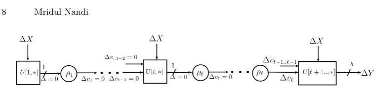
A block matrixU ∈Mn(`, a+`) is called (a, `)-query functionifU[∗, a+ 1..] is block-wise strictly lower triangular. Here`represents the number of queries anda
represents the number of blocks in the input. For any suchquery function, an in-putX∈Ia
n, (and a tuple of`functions ˜ρ= (ρ1, . . . , ρ`) overIn), we canuniquely define or associate u andv, called intermediate input and output vector
respectively, satisfying (1)U · X v
=uand (2) ˜ρ(u) := (ρ1(u1), . . . , ρ`(u`)) =v. This can be easily shown by recursive definitions ofui’s andvi’s. More precisely,
ui is uniquely determined byv1, . . . , vi−1 and X (through the linear function) and vi is uniquely determined byui throughρi, for all 1≤i≤`. Informally, a (a, b, `)-linear mode is a mode which takesablocks input and returns b blocks output based on executing block-functions building blocks (see Fig 1 for an illus-tration of a linear mode). Formally, (a, b, `)-linear mode is defined by a block ma-trixE∈Mn(`+b, `+a) whereE[1..`,∗] is a (a, `)-query function. For any`-tuple of functions ˜ρ∈Func`, the corresponding linear-mode functionEρ˜:Ia
n →Inb is defined asEρ˜(X) =Y where
E·
X v
=
u Y
, ρ˜(u) =v.
ρ1
U[1,∗]
X X
b b b
X
u1 v1 ρ2
v1
uℓ vℓ
u3 Y
ρℓ
X
v1· · ·vℓ−1
u2 v2
U[2,∗] U[3,∗] U[ℓ+ 1..,∗]
b 1
1 1
Fig. 1: Linear Mode: Here U[i,∗] means the ith block row which maps
(X, v1, . . . , vi−1,0`−i+1) to ui. Finally, U[`+ 1..,∗] maps the input X and
interme-diate output vectorvto the outputY consisiting ofbblocks.
Sovis the intermediate output vector associated to the inputXand the final outputY :=E[`+1..,∗]· Xv
, a linear function ofvandX. Now we state an useful differential property of linear mode. Note that the functions of ˜ρare non-linear and would be secret for the adversaries. So to obtain any information about the intermediate input and output, we only can equate intermediate outputs whenever two inputs collide for same function. Given any vectors x, x0 of same size, we write∆xto meanx⊕x0 and∆
a.bxto mean (xa⊕x0a, . . . , xb⊕x0b). We simply write∆txto mean ∆1..tx(the firstt elements of∆x).
Lemma 3. Suppose E[..t,∗]·X = E[..t,∗]·X0 (i.e., E[..t,∗]·∆X = 0). Let
ρ1
U[1,∗] b b b
∆X
∆ = 0 ρt ∆vℓ
ρℓ
∆X
∆vt+1..ℓ−1
U[ℓ+ 1..,∗] ∆Y
b U[t,∗] 1
1
∆v1= 0
∆X
∆vt−1= 0
∆v..t−2= 0
∆ = 0 ∆vt= 0
b b b
Fig. 2: Differential Patterm of the Linear Mode: We choose∆X such that the firstt input differences of theρfunctions are zero. So the final difference∆Y can be expressed as the linear function of the rest of the differences∆vt+1..and∆X.
inputs respectively associated with X and X0 (for the function tuple ρ˜) respec-tively. Then, ∆tu=∆tv= 0t and
∆Y =E[`+ 1.. ; ..a]·∆X+E[`+ 1.. ; a+t+ 1..]·∆vt+1...
Proof. Due to choice of X and X0, by induction one can show that (u 1, v1) = (u0
1, v10), . . .(ut, vt) = (u0t, v0t) where u and u0 denote the intermediate inputs associated withXandX0respectively (for the function tuple ˜ρ). In other words,
∆tu=∆tv= 0t. Now,Y =E[`+ 1..; a+ 1..]·v+E[`+ 1..; ..a]·X and similarly
Y0=E[`+ 1.. , a+ 1..]·v0+E[`+ 1..; ..a]·X0. The result is followed after we add these two equations and using that∆tv= 0t. ut
3.2 Keyed Constructions Based on Linear Mode
Keyed Linear Mode. LetF=F1× · · · × Ff andkbe a non-negative integer where Fi ⊆Func. A key-spaceK for any keyed function is of the form Ink× F. We callF the function-key space and Ik
n masking-key space. Any function g is also written asg+1.
Definition 2. Let µ : [1..`] → [1..f], called key-assignment function, α := (α1, . . . , α`)∈ {+1,−1}`, calledinverse-assignment tuple. For any function-key
ρ= (ρ1, . . . , ρf) ∈ F, we defineραµ := (ραµ11, . . . , ρ α`
µ`). We denote the set of all functionsρα
µ byFµα.
Here we implicitly assume that wheneverαi =−1,ρµi is a permutation. If α= +1`, we simply skip the notationα. In general, the presence of inverse call of building blocks may be required when we consider decryption of keyed function. For the encryption, or a keyed function where decryption is not defined, w.l.o.g. we may assume that α= 1`.
Definition 3. A (k, a, b) keyed linear mode with key-space K, key-assignment functionµ, is a(a+k, b, `)linear modeE. For each keyκ:= (L, ρ)∈ K:=Ik
⊕
u1=p1
ρ1
ua−1=pa−1
⊕
ρa−1
v1 va−1
c1=va
pa
b b b
ua
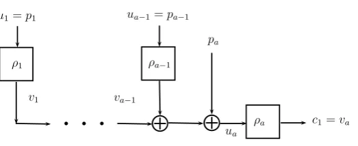
ρa
Fig. 3: The Simplified Structure of PMAC. The input is (p1, . . . , pa) and the output
isc1.
Keyed linear mode E is actually a linear mode with a part of the input is the masking key and function tuples are also derived by reusing some keyed block-functions.
Example 1. Consider the simple variant of PMAC [8, 44] defined over Ia n (see Figure 3 above). Let (p1, . . . , pa) be the input.
1≤i≤a−1, ui=pi andua=pa⊕( a−1 M
i=1
vi).
Finally the output is defined as c1 = va. Here ` = a and b = 1. There is no masking key, i.e.k= 0 andf =a(all function-keys are independently chosen). The key-assignment functionµis an identity function.
In a single function-key version of PMAC (with independent masking key), we have f = 1 =k. Theui =αi·Lfor 1≤i < aandua=pa⊕(La−i=11vi)⊕L. Here the key-assignment function maps all indices to the key-index 1 (as there is only one choice of key).
Affine Domain Extension or ADE [29]. As defined in [29], affine domain extension over Ia
n is nothing but a (a,1, `)-linear mode keyed function E such that the key-space isK=F ⊆Func, i.e., f = 1 (single function-key) andk= 0 (no masking key). Moreover, the final output is the response of the last oracle call, i.e.v`. Like PMAC, the key-assignment function for ADE maps all indices to the key-index 1. One can consider an injective padding rule and sequence of such constructions indexed byato incorporate variable length inputs. CBC-MAC [5], PMAC [8, 24, 32], TMAC [22], OMAC [18, 27], DAG-based constructions [20] etc. are some examples of ADE.
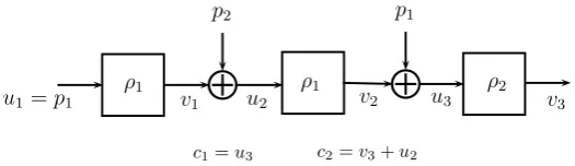
Example 2. As an example, consider Luby-Rackoff (LR) keyed function with three rounds using two random functions ρ1, ρ2, i.e. f = 2, a = b = 2 and
` = 3 (three invocations of the underlying block-functions). Consider the key-assignment function π with π1 = 1, π2 = 1 and π3 = 2. So the function tuple after applying the key-assignment is (ρ1, ρ1, ρ2). As there is no masking key, we have k= 0. So the key-space is Func2. Given (p1, p2)∈In2 we define
u1:=p1, v1=ρ1(u1), u2=v1+p2, v2=ρ1(u2), u3=v2+p1, v3=ρ2(u3).
Finally, the output is (c1, c2) where c1 :=u3 andc2 =v3+u2. This is clearly decryptable. Consider ui’s, vi’s and pi’s as variables. The ciphertext provides two linear functions of these variables, namely u3 andv3+u2. Sou3 is in the span. As u3 is in the span,v3 is also computable. Thusu2 is in the span of the extended ciphertext includingv3. Againv2 is computable and henceu1:=p1 is in the extended span. Finally,p2is in the span after includingv1. So we see that that decryption algorithm is also linear mode.
⊕
u1=p1ρ1
p2
ρ1
⊕
p1
ρ2
u2 u3
v1 v2 v3
c1=u3 c2=v3+u2
Fig. 4:LR with three round.
Decryption Algorithm of a Keyed Linear Encryption Mode. From the above example, it is clear that the intermediate input outputs for the building blocks would be same if we encrypt and then decrypt as we do in the correctness condition: Dκ(Eκ(P)) = P. Informally, if some input-output does not arise in the decryption then either this input-output is redundant in the encryption computation or the correctness condition does not hold (due to randomness of the output which has influence in the encryption but is not used in the decryption). We now describe the details of a length preserving linear encryption mode for which all invocations of block-function calls are not redundant.
Definition 4 (reordering of vectors). Let α:= (α1, . . . , α`)∈ {1,−1}`, and
β = (β1, . . . , β`) be a permutation over [1..`]. A pair of vectors (w, z) ∈ In2` is (a, β)-reordering of a pair of vectors(u, v)∈I2`
n if
(wi, zi) = (
Definition 5. A(k+a, a, `)-linear modeEis calledlinear-mode length-preserving encryption with key-spaceK:=Ik
n× F and key-assignment πif the correspond-ing decryption algorithm D is also a (k+a, a, `)-linear mode with (1) an in-verse assignment-tuple α := (α1, . . . , α`) ∈ {1,−1}` and (2) key-assignment
π0 := π◦β where β = (β
1, . . . , β`) is a permutation over [1..`]. Moreover, ∀P ∈Ia
n, L∈Ink, ρ= (ρ1, . . . , ρf)∈ F,
E·
L P v
=
u C
,ρπ1(u1) =v1, . . . ρπ`(u`) =v` if and only if
D·
L C z
=
w P
,ρα1
π0
1(w1) =z1, . . . , ρ α` π0
`(w`) =z`
where(w, z)is(a, β)-reordering of (u, v).
The above definition implies that correctness condition of an encryption
Dραπ0(L, Eρ(L, P)) = P. In addition with the correctness condition, the
inter-mediate inputs and outputs for both encryption and decryption are simply re-ordered. In Example 2 (given above), we have a = b = f = 2, ` = 3. For the decryption algorithm, we execute the function in the reverse order and so we set β1 = 3, β2 = 2, β1 = 3. So the key-assignment function for the de-cryption is π0
1 = 2, π02 = 2, π30 = 1. We do not need to apply inverse for the decryption (it is called inverse-free) and so inverse-assignment tuple is 13. So if (u1, v1),(u2, v2) and (u3, v3) are the intermediate input-output pairs for encryp-tion then (u2, v3),(u2, v2) and (u1, v1) (reordering of the previous pairs) are the intermediate input-output pairs for decryption.
Examples. EME [16], ELmE [11], AEZ [1], CMC [15] (these follow Encrypt-Mix-Encrypt paradigm), Luby-Rackoff witha=b= 2, unbalanced Fiestel [47, 17] etc. are some examples of length-preserving linear mode encryptions. HCBC1, HCBC2 [3], Modified-HCBC’s, ELmD [1], MCBC [26], COPE [2] etc. are some examples of online computable length-preserving encryptions based on linear mode.
4
PRP and SPRP Distinguishing Attacks
Consider a length-preserving encryption scheme based on (k+a, a, `) linear mode
E. Now we show two main results in this section. Namely, we provide PRP and SPRP distinguishing attacks on the encryption scheme if ` ≤2a−2. and
`≤2a−1 respectively. Thus, it gives lower bound on the number of invocations of building blocks for achieving PRP and SPRP security.
4.1 PRP Distinguishing Attack on E with `= 2a−2
E·
L P v
=
u C
, ρ˜(u) =v.
Distinguisher Dprp against (k+a, a,2a−2)-linear modeE.
1. step-1(finding a suitable difference in a pair of plaintext queries): Letd∈Ia n be the non-zero solution ofsolve(E[..a−1, ..a],0), i.e.E[..a−1 ; k+ 1..k+
a]·d= 0. Such a non-zero solution exists as the number of columns is more than that of rows (see lemma 1).
2. step-2(make the queries with the difference obtained in step-1): Now the distinguisher makes two queries 0a and d and obtains corresponding re-sponsesc=ELρ˜(0) andc0 =Eρ˜
L(d). Let
u1, v1, . . . , u2a−2, v2a−2, andu01, v01, . . . , u02a−2, v02a−2
denote the intermediate inputs outputs for the two queries respectively. By lemma 2, we have 1≤i≤a−1,ui=u0i, vi=vi0 and
∆c=E[2a−1..; k+ 1..(a+k)]·d+E[2a−1..; 2a+k..]·∆va..
while it is interacting with the keyed construction.
3. step-3 (find a nullifier of unknown intermediate values): As the matrix
E[2a−1..; 2a+k..] isa×(a−1) matrix, we find a non-zero binary vec-tor w ∈ {0,1}na such that w
·E[2a−1.. ; 2a+k..] = 0. In particular,
w=solve(E[2a−1..,2a+k..]tr,0).
4. step-4(the distinguisher event): Ifw·∆c=w·E[2a−1..; k+ 1..(a+k)]·d
then it returns 1 (decision for the keyed construction), else returns 0 (decision for uniform random permutation).
The distinguishing advantage of the above distinguisher D is at least 1/2 since for a random permutationw·∆c=w·E[2a−1.. ; k+ 1..(a+k)]·dwith probability 1/2 whereas we have seen this holds with probability one for the keyed construction. When a= 2, we know that LR with three rounds is PRP. This shows the bound is tight at least fora= 2.
A General Distinguisher Dprp against (k+a, a, `)-linear mode E. Now we define a distinguisher against (k+a, a, `)-linear mode E assuming certain singularities in the sub-matrices.
Assumption: Suppose there exists an integert such that
1. rank(E[..t, ..a])< naand
2. rank(E[`+ 1..; a+k+t+ 1..])< na.
Whenever the assumptions hold, we have the following similar distinguisher as mentioned before. This distinguisher would be used later on while describing SPRP distinguishers.
Due to the assumptions. we can finddandwsuch thatE[..t, ..a])·d= 0 and
w·E[`+ 1..; a+k+t+ 1..] = 0. Then we make two queries 0 anddand obtain responsescandc0. The distinguisher returns 1 ifw·∆c=w·E[`+ 1..|k+ 1..(a+
k)]·d, else 0.
4.2 SPRP Distinguishing Attack on E with `= 2a−1
Now we show that if` <2athen we have a SPRP distinguisher. In other words, 2a many invocations is minimum to achieve SPRP and which is tight as it is achieved in CMC. The basic intuition of our attack is similar to that of XLS. However, to complete the attack for any linear-mode encryption we need to carefully set the queries and distinguishing event. Consider a length-preserving (k, a,2a−1)-encryption scheme based on (k+a, a,2a−1)-linear mode E. Let us denote the (k+a, a,2a−1)-linear mode for its decryption byD. We describe three distinguishers depending on cases.
Case 1: rank(E[2a.. ; 2a+k..]) < na
In this case, the two assumptions, mentioned above, hold fort =a−1. So we have our general PRP distinguisher.
Case 2: rank(D[..a ; k+ 1..k+a])< na
In this case, the two assumptions also hold fort=a−1 for the decryption function. So we have our general PRP distinguisher applied to the decryption function works.
Case 3: rank(D[..a ; k+ 1..k+a]) =na, rank(E[2a..; 2a+k..]) =na
Here we describe a SPRP distinguisher. Briefly, it works as follows. It first makes two queries as in step-2 (the first a−1 intermediate input and outputs are identical for two encryption queries). Using the invertible property we can actually obtain all the differences of intermediate values. As the computation of decryption algorithm must use same internal input and outputs of the building blocks, we also know the differences of intermediate inputs and outputs if we decrypt the first two encryption queries. Now we find another decryption query for which the first aintermediate input and output differences with one of the first two queries are fixed. So we can nullify the unknown a−1 differences and obtain a distinguishing event. The details are described below.
1. step-1 (make two queries with a certain difference, same as PRP distin-guisher): Letd∈Ia
n be the non-zero solution ofsolve(E[..a−1 ; ..a],0), i.e.
E[..a−1 ; ..a]·d= 0. It makes two queries 0aanddand obtains corresponding responsesc=ELρ˜(0) andc0=Eρ˜
L(d).
Letu1, v1, . . . , u2a−1, v2a−1 andu01, v10, . . . , u02a−1, v02a−1 denote the interme-diate inputs outputs for the two queries respectively. By lemma 3, we have 1≤i≤a−1,ui=u0i, vi=v0i and
∆c=E[2a−1.. ; k+ 1..(a+k)]·d+E[2a..; 2a+k..]·∆va..
while it is interacting with the keyed construction.
2. step-2(solve for∆u,∆v): Using the invertible property ofE[2a..; 2a+k..], we can actually solve∆va..and hence∆ua... Thus, we know∆uand∆v. Sup-pose we make two (redundant) decryption queriescandc0 (whose responses must be 0 andd) and letw1, z1, . . . , w2a−1, z2a−1andw10, z01, . . . , w20a−1, z20a−1 denote the intermediate inputs outputs for the two queries respectively. Then by the definition of decryption algorithm we also know∆w, ∆z which are nothing but (β, π)-reordering of (∆u, ∆v).
3. step-3 (find a difference for the final decryption query): Now we find a differenced0 such that
D[..a; k+ 1..k+a+ 1]· d0
∆z1
= ∆w
1 0a−1
.
We can solve for a non-zerod0. This can be solved assuming that ∆w 16= 0 (see the remark below). Note that the matrixD[..a; k+1..k+a] is invertible. Now we make two decryption queries ¯c and ¯c0 = ¯c+d0. While we set two queries we should ensure that none of these have been obtained in the first two encryption queries (these are also called non-pointless or non-trivial queries). Let ¯w1,z¯1, . . . ,w¯2a−1,¯z2a−1 w¯01,z¯10, . . . ,w¯20a−1,z¯02a−1denote the in-termediate inputs outputs for these two queries respectively and let ¯p and ¯
p0 denote the corresponding responses. By choice ofd0 we know that ¯z 1= ¯z10 and∆z¯2..a= 0a−1.
4. step-4 (find a nullifier of unknown intermediate values, same as PRP dis-tinguisher): AsD[2a.. ; 2a+k..] isa×(a−1) matrix, we find a non-zero binary vectorw∈ {0,1}nb such thatw
·D[2a..,2a+k..] = 0.
5. step-5(the distinguisher event): Ifw·(¯p⊕p¯0) =w·D[2a−1..; k+1..(a+k)]·d0 then it returns 1 (decision for the keyed construction), else returns 0 (decision for uniform random permutation).
Remark 1. In the above attack we assume that ∆w1 6= 0 since otherwise we do not get a non-zero d0. Note that∆w
1 can be written as a function ofc and
5
Security Analysis of Inverse-free Single Key
Construction
5.1 PRP Attack of Single-Key Inverse-free Constructions without Masking
In the last section, we have seen that to obtain PRP, we need at least 2a−1 invocations and this is tight as three rounds of LR achieves this bound. Note that the three calls of the building block can not have same key. In [28], it is also shown that three rounds of LR-type rounds with same key building block can not be PRP. However, their result is applicable to a specific form of encryption schemes. Now, we generalize this result and show that any inverse-free single function-key (and no masking key) PRP requires at least 2acalls. In [28], there is a construction of inverse-free SPRP over two blocks invoking underlying function (single keyed) four times. So the bound is tight. Interestingly, the cost of PRP and SPRP become same when we want inverse-free single function-key constructions. Consider a length-preserving encryption scheme based on (a, a,2a−1)-linear modeE. Let us denote the (a, a,2a−1)-linear mode for its decryption byD. Since it is inverse-free the inverse-assignment for the decryption is β = (1,1, . . . ,1). As it is based on single function-key, the key-assignment is a constant function, i.e., πi = πi0 = 1. However, there exists a permutation β over [1..2a−1]. such that w and z are π-reordering of u and v respectively where u, v denote the intermediate input and output, respectively forEρ(P) =Cand similarlyw, zfor
Dρ(C) =P. We first briefly describe how we can construct a PRP-distinguisher (as like SPRP). The attack is similar to SPRP but we can not make decryption queries. We see how we can manage even if we are not allowed to make decryption queries.
We make two encryption queries such that∆a−1u=∆a−1v= 0a−1. This is possible as we haveamany plaintext blocks. Assuming some invertible property, we can find out the whole differences∆uand∆vfor these two queries. For these two queries, if we look at the decryption computation then the first inputs, say
w1, w01 and their corresponding output differences∆z1 (not the exact outputs) for both decryption are known (as there is no masking key). So now we make two encryption queries with the the following restrictions on intermediate values
u, v, u0 andv0:u1=w1, u01=w10,∆2..au=∆2..au0,∆2..av=∆2..av0. As we have obtained differences for the firstainputs in a determined manner, we can nullify the remaininga−1 intermediate differences and obtain a distinguishing event. The more details of the attack is given below depending on different cases. Note that the matrixE∈Mn(3a−1,3a−1).
Case 1: rank(rankE[2a.. ; 2a..]) < na In this case, the two assumptions, mentioned before, hold fort=a−1. So we have our general PRP distinguisher.
Case 3: rank(rankE[1..a ; ..a]) = na, rank(rankE[2a.. ; 2a..]) = na
Here we describe a PRP distinguisher which works similar to SPRP distinguisher and as described above.
DistinguisherDprpagainst(a, a,2a−1)-linear-modeE(with
correspond-ing decryption modeD.
1. step-1 (make two queries with a certain difference, same as PRP distin-guisher): Letd∈ Ia
n be the non-zero solution of solve(E[..a−1, ..a],0), i.e.
E[..a−1, ..a]·d= 0. It makes two queries 0aanddand obtains corresponding responsesc=Eρ(0) andc0=Eρ(d).
Letu1, v1, . . . , u2a−1, v2a−1 andu01, v10, . . . , u02a−1, v02a−1 denote the interme-diate inputs outputs for the two queries respectively. By lemma 3, we have 1≤i≤a−1,ui=u0i, vi=v0i and
∆c=E[2a−1..|k+ 1..(a+k)]·d+E[2a..,2a+k..]·∆va..
while it is interacting with the keyed construction.
2. step-2(solve for∆u,∆v): Using the invertible property ofE[2a..,2a..], we can actually solve∆va..and hence∆ua... Thus, we know∆uand∆v. Now note that the first input of decryption D is only based on c and c0. Let β be the permutation corresponding to the reordering of intermediate input outputs for decryption. So the values of uβ1 and u
0
β1 are known (as they depend only oncandc0 due to no masking keys and inverse-free property). Moreover, we know∆vβ1. Here we assume the difference∆uβ1 is non-zero, otherwise, we can have a different distinguishing event as zero difference can occur with low probability for random permutation.
3. step-3 (find a difference for two more encryption queries): Now we find a solutionpandp0 such that
E[1,∗] 0 0 E[1,∗]
E[2..a,∗]E[2..a,∗]
·
p p0
=
uβ1
u0 β1 0
.
This can be solved as it has full column rank (see Lemma 2). Now we make two encryption queriespandp0 and obtain outputscandc0. Letu, v, u0 and
v0 be the intermediate inputs and outputs for these two queries respectively. So u1 = uβ1, u
0
1 = u0β1, ∆v1 = ∆vβ1 and ∆2..au = ∆2..av = 0
a−1. Thus, thea block output difference∆c depends only on the a−1 blocks of the intermediate output difference∆va+1...
4. step-4(find a nullifier of unknown intermediate values, same as PRP distin-guisher): AsE[2a..,2a+ 1..] isa×(a−1) matrix, we find a non-zero binary vectorw∈ {0,1}nb such thatw
·E[2a..,2a+ 1..] = 0.
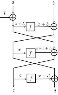
5.2 PRP security of Single-Key Luby-Rackoff with Masking
Define one round Luby-Rackoff LRf(a, b) = (b⊕f(a), a) where a, b ∈ In and
f ∈ Func(a, a). In [28] it was shown that three rounds of some variants LR rounds with single function key is not PRP secure. In last section we have also generalized and showed that any encryption making three calls over two blocks input with key space K =F = Func(a) is not PRP secure. However, we now show that a simple variant of LR with a masking key becomes PRP secure.
Definition 6. For any f ∈Func(a),L∈In, we define
LRf,L3(a, b) =LRf(LRf(LRf(a+L, b))).
⊕
a
⊕
b
⊕
⊕
c d
L
f
f
f x
a+L x+b
x+d
a+c+L
c
Fig. 5:LR-three rounds single function-key and one masking key.
Now we show that the above construction with key-spaceK=In×Func is PRP. Note that we have constant key-assignment (i.e., we reuse the PRF for all invocations) and also inverse assignment tuple is 13. Letf denote the uniform random function on In. Given a tuple of elements c = (c1, . . . , ct) we say that the eventcoll(c) holds if there exitsi6=j such thatci=cj. We define
Vbad={((a1, b1, c1, d1), . . .(aq, bq, cq, dq))∈In4q :coll(c)}.
It is easy to see that for random functionΓ2 and aq-algorithmA,
Pr[τ(AΓ2)
∈ Vbad]≤
q
2
Now we show the high interpolation probability of the variant of 3 round LR construction.
Proposition 1. For all((a1, b1, c1, d1), . . .(aq, bq, cq, dq))6∈ Vbad, we have
Pr[LRf,L3(ai, bi) = (ci, di),1≤i≤q]≥(1−)2−2nq
where= 2q(q−1)2−n.
Proof.We say that a tuple (L0,(xi)1≤i≤q) isadmissibleif 1. L06∈ {ai+cj; 1≤i, j≤q} ∪ {ai+xj; 1≤i, j≤q}, 2. xi’s are distinct andxi6=cj, 1≤i, j≤qand 3. wheneverai=aj, we havexi+xj =bi+bj.
LetAdenote the set of admissible tuples. Let q1 be the number of distinct
ai’s. The number of (L0, x= (x1, . . . , xq)), denotedN1,3, satisfying only (1) and (3) is at least (2n
−q(q−1))×2nq1. So the number of admissible tuple is at least (2n
−q(q−1))×2nq1 −(2n
−q(q−1))×2n(q1−1)q(q −1).
We mainly subtract the number of tuples satisfying (1) and (3) and not satisfying (2) fromN1,3. So the number of admissible tuple is at least 2n(q1+1)(1−) where
=q(q−1)2−n+1.
Now, for anyτ= ((a1, b1, c1, d1), . . .(aq, bq, cq, dq))6∈ Vbad we have
Pr[τ]≥ X (L0,x)∈A
Pr[τ, Xi=xi, L=L0] = X
(L0,x)∈A
2−n(q1+2q+1).
By using the lower bound of the number of admissible tuples we have
Pr[LRf,L3(ai, bi) = (ci, di),1≤i≤q]≥(1−)2−2nq
where= 2q(q−1)2−n.
u t
Theorem 2. For any q-adversary, the PRP advantageAdvprp
LRf,L3 against LR
f,3 L
is at most 2.5q2(nq−1).
Proof.Armed with the above result and using Coefficient-H technique the
the-orem follows. ut
6
Conclusion
requires at leat 2`−1 blockcipher calls against chosen plaintext adversaries and at least 2`blockcipher calls against chosen plaintext-ciphertext adversaries. This bounds are clearly tight as we know some constructions achieving the bound. Then we look into inverse-free single-key PRP constructions. Nandi has shown that three blockcipher call is no longer sufficient for LR-type constructions over two blocks (note that three call is sufficient using two independent PRF). We extend this result and show that any `-block single-key inverse-free PRP must require 2` calls like SPRP constructions. However, if we are allowed to use one masking key then we can have inverse-free PRP construction invoking only three blockcipher calls. We actually show that the three round LR using same keyed PRF is PRP if we mask a plaintext block by a masking key.
Acknowledgement. The author would like to thank Lear Bahack who found an error of the SPRP distinguisher in one of the sub-cases. Author is also grate-ful to Lear for pointing out the unpublished claim in the submission draft of authenticated encryption Julius.
References
1. CAESAR submissions, 2014. http://competitions.cr.yp.to/caesar-submissions.html.
2. Elena Andreeva, Andrey Bogdanov, Atul Luykx, Bart Mennink, Elmar Tis-chhauser, and Kan Yasuda. Parallelizable and authenticated online ciphers. In Kazue Sako and Palash Sarkar, editors, Advances in Cryptology - ASIACRYPT 2013 - 19th International Conference on the Theory and Application of Cryptology and Information Security, Bengaluru, India, December 1-5, 2013, Proceedings, Part I, volume 8269 of Lecture Notes in Computer Science, pages 424–443. Springer, 2013.
3. M. Bellare, A. Boldyreva, L. Knudsen, and C. Namprempre. On-line ciphers and the hash-cbc constructions. InAdvances in Cryptology –Crypto 2001, number 2139 in Lecture Notes in Computer Science, pages 292–309, Berlin, 2001. Springer. 4. M. Bellare and P. Rogaway. The security of triple encryption and a framework
for code-based game-playing proofs. InAdvances in Cryptology – Eurocrypt 2006, number 4004 in Lecture Notes in Computer Science, pages 409–426, Berlin, 2006. Springer.
5. Mihir Bellare, Joe Kilian, and Phillip Rogaway. The security of cipher block chain-ing. In Yvo Desmedt, editor,CRYPTO, volume 839 ofLecture Notes in Computer Science, pages 341–358. Springer, 1994.
6. Thierry P Berger, Marine Minier, and Ga¨el Thomas. Extended generalized feistel networks using matrix representation. In Selected Areas in Cryptography–SAC 2013, pages 289–305. Springer, 2014.
7. Daniel J. Bernstein. A short proof of the unpredictability of cipher block chaining (2005).
FSE 2008, Lausanne, Switzerland, February 10-13, 2008, Revised Selected Papers, volume 5086 ofLecture Notes in Computer Science, pages 289–302. Springer, 2008. 10. Joan Daemen and Vincent Rijmen. The Design of Ri-jndael: AES - The Advanced Encryption Standard., 2002. http://csrc.nist.gov/CryptoToolkit/aes/rijndael/Rijndael-ammended.pdf.
11. Nilanjan Datta and Mridul Nandi. Misuse resistant parallel authenticated encryp-tions. IACR Cryptology ePrint Archive, 2013:767, 2013.
12. Oded Goldreich, Shafi Goldwasser, and Silvio Micali. How to construct random functions. J. ACM, 33(4):792–807, August 1986.
13. Shai Halevi. EME*: Extending EME to handle arbitrary-length messages with associated data. In Anne Canteaut and Kapalee Viswanathan, editors, IN-DOCRYPT, volume 3348 ofLecture Notes in Computer Science, pages 315–327. Springer, 2004.
14. Shai Halevi. Invertible Universal Hashing and the TET Encryption Mode. In Alfred Menezes, editor, CRYPTO, volume 4622 of Lecture Notes in Computer Science, pages 412–429. Springer, 2007.
15. Shai Halevi and Phillip Rogaway. A tweakable enciphering mode. In Dan Boneh, editor,CRYPTO, volume 2729 ofLecture Notes in Computer Science, pages 482– 499. Springer, 2003.
16. Shai Halevi and Phillip Rogaway. A parallelizable enciphering mode. In Tatsuaki Okamoto, editor, CT-RSA, volume 2964 of Lecture Notes in Computer Science, pages 292–304. Springer, 2004.
17. Viet Tung Hoang and Phillip Rogaway. On generalized feistel networks. In Ad-vances in Cryptology–CRYPTO 2010, pages 613–630. Springer, 2010.
18. T. Iwata and K. Kurosawa. Omac: One-key cbc mac. In Fast Software Encryp-tion, 10th International Workshop – FSE 2003, number 2887 in Lecture Notes in Computer Science, pages 129–153, Berlin, 2003. Springer.
19. Tetsu Iwata and Kan Yasuda. Btm: A single-key, inverse-cipher-free mode for deterministic authenticated encryption. InSelected Areas in Cryptography, pages 313–330. Springer, 2009.
20. C. S. Jutla. Prf domain extension using dag. In Theory of Cryptography: Third Theory of Cryptography Conference – TCC 2006, number 3876 in Lecture Notes in Computer Science, pages 561–580, Berlin, 2006. Springer.
21. CharanjitS. Jutla. Lower bound on linear authenticated encryption. In Mitsuru Matsui and RobertJ. Zuccherato, editors,Selected Areas in Cryptography, volume 3006 of Lecture Notes in Computer Science, pages 348–360. Springer Berlin Hei-delberg, 2004.
22. K. Kurosawa and T. Iwata. Tmac: Two-key cbc mac. InTopics in Cryptology – CT-RSA 2003: The Cryptographers’ Track at the RSA Conference 2003, number 2612 in Lecture Notes in Computer Science, pages 33–49, Berlin, 2003. Springer. 23. M. Luby and C. Rackoff. How to construct pseudo-random permutations from
pseudo-random functions. InAdvances in Cryptology – Crypto 1985, number 218 in Lecture Notes in Computer Science, page 447, New York, 1984. Springer-Verlag. 24. K. Minematsu and T. Matsushima. New bounds for pmac, tmac, and xcbc. In
Fast Software Encryption – FSE 2007, number 4593 in Lecture Notes in Computer Science, pages 434–451, Berlin, 2007. Springer.
26. Mridul Nandi. Two new efficient cca-secure online ciphers: Mhcbc and mcbc. In Di-panwita Roy Chowdhury, Vincent Rijmen, and Abhijit Das, editors,INDOCRYPT, volume 5365 ofLecture Notes in Computer Science, pages 350–362. Springer, 2008. 27. Mridul Nandi. Improved security analysis for OMAC as a pseudorandom function.
J. Mathematical Cryptology, 3(2):133–148, 2009.
28. Mridul Nandi. The characterization of luby-rackoff and its optimum single-key variants. In Guang Gong and Kishan Chand Gupta, editors,INDOCRYPT, volume 6498 ofLecture Notes in Computer Science, pages 82–97. Springer, 2010.
29. Mridul Nandi. A unified method for improving PRF bounds for a class of block-cipher based macs. In Seokhie Hong and Tetsu Iwata, editors,Fast Software En-cryption, 17th International Workshop, FSE 2010, Seoul, Korea, February 7-10, 2010, Revised Selected Papers, volume 6147 ofLecture Notes in Computer Science, pages 212–229. Springer, 2010.
30. Mridul Nandi. On the minimum number of multiplications necessary for universal hash functions. In Carlos Cid and Christian Rechberger, editors, Fast Software Encryption - 21st International Workshop, FSE 2014, London, UK, March 3-5, 2014. Revised Selected Papers, volume 8540 ofLecture Notes in Computer Science, pages 489–508. Springer, 2014.
31. Mridul Nandi. XLS is not a strong pseudorandom permutation. In Palash Sarkar and Tetsu Iwata, editors,Advances in Cryptology - ASIACRYPT 2014 - 20th Inter-national Conference on the Theory and Application of Cryptology and Information Security, Kaoshiung, Taiwan, R.O.C., December 7-11, 2014. Proceedings, Part I, volume 8873 ofLecture Notes in Computer Science, pages 478–490. Springer, 2014. 32. Mridul Nandi and Avradip Mandal. Improved Security Analysis of PMAC.
Cryp-tology ePrint Archive, Report 2007/031, 2007. http://eprint.iacr.org/.
33. Moni Naor and Omer Reingold. A pseudo-random encryption mode. Manuscript available from www.wisdom.weizmann.ac.il/˜naor.
34. Moni Naor and Omer Reingold. On the construction of pseudorandom permuta-tions: Luby-Rackoff revisited. J. Cryptology, 12(1):29–66, 1999.
35. J. Patarin. Etude des G´en´erateurs de Permutations Bas´es sur le Sch´ema du D.E.S. Phd Th`esis de Doctorat de l’Universit´ede Paris 6, 1991.
36. Jacques Patarin. New results on pseudorandom permutation generators based on the des scheme. InAdvances in Cryptology?CRYPTO?91, pages 301–312. Springer, 1992.
37. Jacques Patarin. How to construct pseudorandom and super pseudorandom permutations from one single pseudorandom function. In Advances in Cryptol-ogy?EUROCRYPT?92, pages 256–266. Springer, 1993.
38. Jacques Patarin. Generic attacks on feistel schemes. In Advances in Cryptolo-gyASIACRYPT 2001, pages 222–238. Springer, 2001.
39. Jacques Patarin. Security of random feistel schemes with 5 or more rounds. In
Advances in Cryptology–CRYPTO 2004, pages 106–122. Springer, 2004.
40. Jacques Patarin. The ?coefficients h? technique. InSelected Areas in Cryptography, pages 328–345. Springer, 2009.
41. Josef Pieprzyk. How to construct pseudorandom permutations from single pseudo-random functions. In Advances in Cryptology?EUROCRYPT?90, pages 140–150. Springer, 1991.
42. Thomas Ristenpart and Phillip Rogaway. How to enrich the message space of a cipher. In Alex Biryukov, editor,FSE, volume 4593 ofLecture Notes in Computer Science, pages 101–118. Springer, 2007.
44. Phillip Rogaway. Efficient instantiations of tweakable blockciphers and refinements to modes ocb and pmac. In Pil Joong Lee, editor, ASIACRYPT, volume 3329 of
Lecture Notes in Computer Science, pages 16–31. Springer, 2004.
45. Babak Sadeghiyan and Josef Pieprzyk. A construction for super pseudorandom permutations from a single pseudorandom function. In Advances in Cryptol-ogy?EUROCRYPT?92, pages 267–284. Springer, 1993.
46. Palash Sarkar. Improving upon the tet mode of operation. In Kil-Hyun Nam and Gwangsoo Rhee, editors, ICISC, volume 4817 of Lecture Notes in Computer Science, pages 180–192. Springer, 2007.
47. Bruce Schneier and John Kelsey. Unbalanced feistel networks and block cipher design. InFast Software Encryption, pages 121–144. Springer, 1996.
![Fig. 1:Lineardiate output vector(Mode:HereU[i, ∗]meanstheithblockrowwhichmapsX, v1, .](https://thumb-us.123doks.com/thumbv2/123dok_us/7937079.1317736/7.595.142.498.354.467/fig-lineardiate-output-vector-mode-hereu-i-meanstheithblockrowwhichmapsx.webp)