Study the Trend Pattern in COVID-19 using Spline-Based Time Series Model: A Bayesian Paradigm

(1)

Study the Trend Pattern in COVID-19 using Spline-Based Time Series Model:

A Bayesian Paradigm

Varun Agiwal1, Jitendra Kumar2,* and Yau Chun Yip3

1_{Department of Community Medicine, Jawaharlal Nehru Medical College, Ajmer, India}

2_{Department of Statistics, Central University of Rajasthan, Ajmer, India}

3_{Department of Statistics,}_{Chinese University of Hong Kong, Hong Kong}

Email: [email protected], [email protected] and [email protected]

Abstract

A vast majority of the countries is under the economic and health crises due to the current

epidemic of coronavirus disease 2019 (COVID-19). The present study analyzes the COVID-19

using time series, which is an essential gizmo for knowing the enlargement of infection and its

changing behavior, especially the trending model. We have considered an autoregressive model

with a non-linear time trend component that approximately converted into the linear trend using

the spline function. The spline function split the COVID-19 series into different piecewise

segments between respective knots and fitted the linear time trend. First, we obtain the number

of knots with its locations in the COVID-19 series and then the estimation of the best-fitted

model parameters are determined under Bayesian setup. The results advocate that the proposed

model/methodology is a useful procedure to convert the non-linear time trend into a linear

pattern of newly coronavirus case for various countries in the pandemic situation of COVID-19.

Keywords: COVID-19, Linear and non-Linear trend, Spline function, Autoregressive Time series model, Bayesian inference

*Corresponding Author: Dr. Jitendra Kumar, Associate Professor, Department of Statistics, Central University of Rajasthan, Ajmer, India, Email: [email protected]

(2)

1. Introduction

The 2019 novel coronavirus (COVID-19) is getting a lot of attention now because it is a new

kind of pandemic disease that affects most of the world. Lakhs of the people have died from this

disease, and lakhs of cases are recorded in worldwide because of the nonexistence of antiviral

drugs and vaccines. Researchers developed various methodologies to analyze and control the

spreading of COVID-19 and predictive the future perspective of coronavirus cases. Jiang et al.

(2020) established the time series and kinetic model for infectious diseases and predicted the

trend and short-term prediction of the transmission of COVID-19. AL-Rousan and AL-Najjar

(2020) analyzed the effect of various factors such as sex, region, infection reasons and birth year

on recovered and deceased cases of the South Korea region. The results found that sex, region,

and infection reasons affected on both recovered and deceased cases, while birth year only

affected on deceased cases. Gondauri et al. (2020) considered the chain-binomial type of

Bailey’s model for studying and analyzing the correlation between the total volumes of

COVID-19 virus spread and recovery from the different countries. Most of the study investigates the

COVID-19 cases based on various regression and time series models because these models are

frequently applied to examine the growth or trend of any disease.

In the COVID-19 series, the newly recorded cases having non-linear characteristics and shows a

non-trend pattern that occurred in each country and the process has drawn a non-stationary

series. This non-linear trend may be model in COVID-19 by piecewise time series model with a

high order of polynomial-time pattern. Spline function is the alternative to deals such as

piecewise time trend polynomial. It is analyzed period wise discontinuity by fitting a polynomial

of a high order and joined at knots. Knots are the points when there are sudden up and down in

the trends of series and resulting piecewise smooth time function. Eubank (1999) observed that

the smoothest piecewise polynomials is a spline function that holds a segmented nature at

present, but Hurley et al. (2006) called splines as continuous and smooth lines or curves function.

Morton et al. (2009) considered a smoothing spline function to analyze the trend of generalized

additive models with correlated errors and applied to data from a chemical process and to stream

salinity measurements. Montoril et al. (2014) studied the estimation of functional-coefficient

(3)

the proposed estimator. Qiao et al. (2015) conducted a B-spline modeling study on the durability

of changes in the frequency signal over time. Conrad et al. (2017) modeled the forced expiratory

volume 1 (FEV1) data from cystic fibrosis (CF) and chronic obstructive pulmonary disease

(COPD) using median regression splines. Osmani et al. (2019) used the B-spline and kernel

methods to estimate the coefficient in rates model and showed its application for psoriasis

patient’s data.

In this paper, we study the trend pattern of COVID-19 series using an autoregressive model with

a trend approximated by a linear spline function. Identification of the number of knots and their

location is obtained using posterior probability. We use appropriate priors of model parameters

for deriving the posterior distribution and find the conditional posterior distribution for making

inference about the parameters. We apply the Metropolis–Hasting (M-H) algorithm within

Gibbs sampler to generate posterior samples and get the Bayesian estimation for unknown

parameters. The study would give an overview of the present trend of new recorded COVID-19

cases in the most affected countries and shows the changing pattern in different segments.

2. Model specification

A time series model is popularly known to regulate the trend pattern for the series of coronavirus

(COVID 19). We observed that the series has a non-linear trend component in newly recorded

cases of COVID-19. This non-linear trend function can be controlled its non-linearity in the time

series using the spline function. Recently, this model is discussed by Kumar et al. (2020) for

testing the unit root hypothesis in the presence of spline function through posterior odds ratio and

applied in monthly import series of ASEAN Regional Forum (ARF) countries. The complete

detail about this model well described in Kumar et al. (2020). Here, we only write the key

expression of the model. Let {yt : t = 1 , 2 , … ,T} is time series from the model





t

r

i

i i

i t

t y t s t s t

y = − + + +



 − − +

= −

1

1 ( ) ( 1)

) 1

(

(4)

knot, εt’s are i.i.d. normally distributed random variables with mean zero and unknown variance

-1_and_s

i(t) is a spline function describe as a linear polynomial form defined as follows:

(

)

     − = − = + i i i i i t t if t t if t t t t t s 0 ) (

In the existing literature, researchers do the modeling of COVID-19 series based on various

regression and time series models but they ignore the irregular behaviour of daily-conformed

cases of the COVID-19 as most of the countries take necessary steps to control the spread of

COVID-19. These steps change the growth of COVID-19 cases in up and down manner. As a

result, the trend pattern is not linear form and there is an occurrence of sudden jumping

phenomena in COVID-19 series. Thus, there is a need to apply some other non-linear models

that provide better results for this situation. The proposed model is one of the best suitable

models to analyze the non-linear trend pattern of the COVID-19 series because this model split

the series into a linear form at their knot locations.

In matrix notations, the model is marked as

      + + +

= y₋₁ Z( ) S( )

y

(

1 2

)

,

= T

T 

The main objective is to study the tendency of daily conformed COVID-19 cases by fitting this

model in a piecewise form and understand the increases of infection. For this, first determine the

number of knots with their location in COVID-19 series using posterior probability, and then

estimators of the model parameters are derived using conditional posterior distribution.

3. Bayesian estimation

For analysis purposes, Bayesian approach is used to make inference about the unknown

parameter and drawn a better conclusion. In Bayesian approach, the posterior for all unknowns is

proportional to the product of the likelihood and prior distributions. Here, the discrete uniform

prior is assumed for location of knots under consideration of all ordered subsequences (2, 3,..., T)

of length r, i.e., 

(

t_i |r

)

=T−1C_r. The number of knots follows a Binomial (T-1, p) distribution,

and the remaining model parameters consider similar prior information’s as described in Kumar

et al. (2020). Then, the posterior specification for this model is as

follow

( )



(

( )

)

(

( )

)

(

) (

)

(

)

_

     −

− −

− + −  − +

− −

− 

₋ ₋ ₋ ₋

 

 ₋ ₋

+ + −

+

0 '

0 0

' 0

1 '

1 1

2 1

2 1 2

1 2

) 1 ( ) ( ) 1 ( 2

exp

) 2 (

) (

  

   

  



    



  



V

S Z

y y S

Z y y C

V

y _T _r

r T

For Bayesian parameter estimation, a loss function is used to select the best estimator from the

posterior distribution that minimizes the loss incurred for the estimation. Here, we consider

squared error loss function (SELF) as a symmetric loss function. Under this loss function,

Bayesian estimator for a parameter is posterior mean. A computational approach such as the

Markov chain Monte Carlo (MCMC) technique is applied for obtaining the estimators because it

contains multiple integrals that cannot be solved without any computational method. For that, we

derived the conditional posterior distribution/ probability of model parameters.

(

)

(

₍

₎

)

r y

r y t r y

t_i i

| | , ,

|

 

(6)

(

)



(

( )

)

(

( )

)

(

)

(

)

_      − − − − + − − −  ₋ ₋ ₋ ₋ = ₋ ₋ 0 ' 0 1 ' 1 2 1 ) 1 ( ) ( ) 1 ( 2 exp ) ( , , , |                         V S Z y y S Z y y V y

( )

(

( )

)

(

)

( ) ( )

(

)

(

( ) ( )

)

       ₊ + − + − − ₋ −                   1 ' ' 0 1 ' ) ( , ) ( ) ( ) 1 ( ~ , , ,

| Z Z V

V Z Z V S y y Z MN y

( )

(

( )

)

(

)

( ) ( )

(

( ) ( )

)

       ₊_  +  + − − ₋ −               1 ' ' 0 1 ' , ~ , , ,

| S S

S S Z y y S MN y where

(

)

(

)

(

)





( )

(

)

( )

(

)

( )

(

)

( )

(

)

( )

(

)

(

( )

) (

)

(

)

(

0

)

' 0 0 ' 0 1 ' 1 1 ' 0 1 ' 0 ' 1 ' 1 0 ' 0 2 1 ' 1 0 1 1 1 1 2 2 1 2 1 2 3 2 1 1 ) 1 ( ) ( ) 1 ( ) ( ) ( ) ( ' ) ( ) ( 2 ) ( ) 1 ( ) )( ( ) ( ) ( ) ( ) ( ) 1 ( ) )( ( ) ( ' ) ( ; ) ( ) ( ) ( ' ) ( ) ( ' ) ( ) ( ) ( ; ) ( ) ( ' ) ( | , | ; ) ( ) ( ) ( 1 1 1 | , 1                                                                         − − − − + −  − + − − − − − − =  −   −  +  − − − + − − =  − + + − = + = − =  + = = − +  − − − − − − − − − − − −



 

V S Z y y S Z y y C D C A A S y y V y y B y y A S Z y y B Z C V Z B Z D S A S I B S S A r y t r y d D A C r y t o o o o t t i a T r T i r 

The location of knots and autoregressive coefficient are not in closed distribution form. So, the

M-H algorithm is applied to draw samples from the posterior distribution, whereas remaining

parameters generate posterior samples from the Gibbs sampler algorithm because conditional

posterior distribution is coming in close distribution. The number of knots is determined by using

Bayes factor. The Bayes factor (BFn,m) is the ratio of one versus another model/hypothesis, i.e., it

is determined by the posterior probability of n knots divided by m knots. For this model, BFn,m is

expressed as       + ₊  2 , 1 2 ~ , , ,

|y    Gamma T r

(7)

(

)

(

)

(

)

(

)

 

= =

1 1

| ,

| | ,

t t i t t

i m

n

m n

m y t

n y t

m r y

n r y BF

 

 

The procedure is started with the series has no knot and evaluate the evidence to support for one

or more knots. If there is a significant evidence for supporting the existence of knots then check

whether there are one knot, two knots or so on. So, our aim is to find at least strong evidence

between the models/hypotheses before getting a better decision about the number of knots.

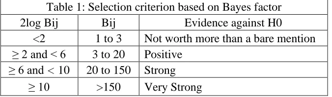
Kass and Raftery (1995) provided a rule of thumb for interpreting the magnitude of a Bayes

factor using the transformation 2loge(BFn,m) in Table 1 and put on the same scale as the

likelihood ratio.

Table 1: Selection criterion based on Bayes factor

2log Bij Bij Evidence against H0

<2 1 to 3 Not worth more than a bare mention ≥ 2 and < 6 3 to 20 Positive

≥ 6 and < 10 20 to 150 Strong

≥ 10 >150 Very Strong

Another approach is to find out the number of knots by using an information criterion that is well

discussed by Kumar et al. (2020).

4. Modeling of COVID-19 series

We have collected the COVID-19 data from the World Health Organization’s official daily

reports. The data covers the number of people infected daily by COVID-19. Due to the limitation

of the study and the number of cases recorded, we modeled most affected countries and found

out the growth structure by fitting the proposed model. The study analyzes to start from 100

outbreaks of corona cases and equal to the date on 31st May 2020 for the selected countries. In

our study, the number of confirmed cases has been rising, increasing at a rapid rate. Then, the

spread of the virus has slowed down in most of the selected countries such as Italy, Spain, the

United Kingdom, etc.

In contrast, some countries like India, United States, Brazil, etc. have a rapid growth of infected

(8)

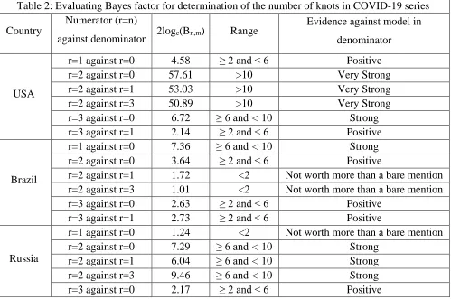
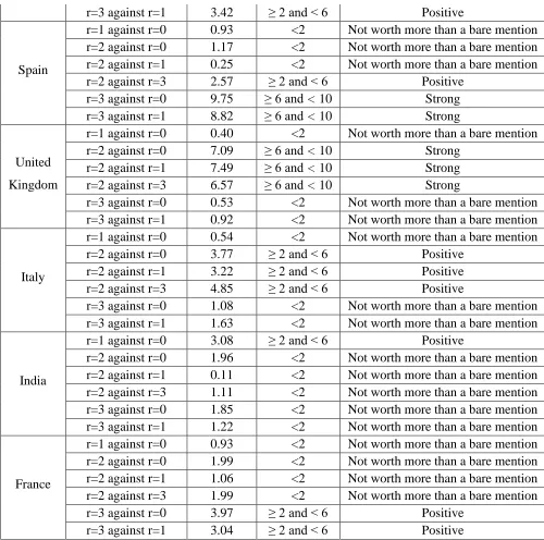
where the growth of the stage of COVID-19 cases is changed and the results record in Table 2.

From Table 2, one can observe that model with r = 2 knots is better than the model with r=0,1 and 3 knots for the USA country as the corresponding value of 2loge(BFn,m) is greater than 10. It

indicates that there is robust evidence in favor of r = 2 against r = 0, 1, 3 for the given COVID-19 USA series. The following countries Russia, United Kingdom and Italy have also obtained

the model with r = 2 knots because strong and positive evidence in favor of r = 2 is recorded in comparison to r= 0, 1, and 3 knots. For Spain and France countries, a maximum of three knots

(r=3) are presented to fit the model with a linear trend pattern in the series as these countries

control the confirmed COVID cases in the early stage of coronavirus. So, the first knot is

happened in the early days, i.e., near to higher peak, and then the remaining two knots are

presented in the downward trend as it has an extended tail area after a higher peak. In the present

study period, only two countries (India and Brazil) record the number of confirmed cases in a

rapidly increasing pattern and do not achieve a high peak. So, the best-fitted model has only one

knot (r=1) as Bayes factor values lie in between 2 to 6. Hence, strong evidence is found in favor

of a model with one knot as compared to a model with more than one knot.

Table 2: Evaluating Bayes factor for determination of the number of knots in COVID-19 series

Country

Numerator (r=n)

against denominator

model (r=m)

2loge(Bn,m) Range Evidence against model in denominator

USA

r=1 against r=0 4.58 ≥ 2 and < 6 Positive

r=2 against r=0 57.61 >10 Very Strong

r=3 against r=0 6.72 ≥ 6 and < 10 Strong

Brazil

r=2 against r=1 1.72 <2 Not worth more than a bare mention

Russia

(9)

Spain

United

Kingdom

Italy

India

France

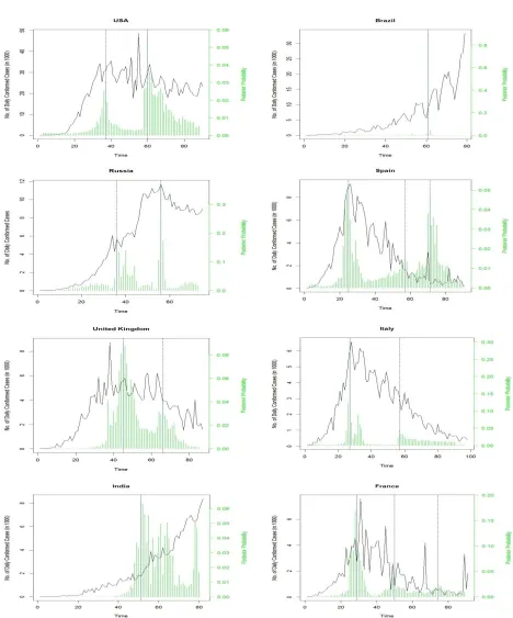
Once the suitable number of knots in each study country is determined, the location of the knot is

found based on derived posterior probability. The values of posterior probability display in

(10)

Figure 1: Selection of knot location(s) based on the posterior probability

Based on Figure 1, the first joint point select by considering every time point in the interval (2,

T-r) as a knot point and record the probabilities that occur parallel to these points. The study

(11)

point. The second-knot location is determined in the interval

(

tˆ₁+1,T −r+1

)

where it records the

maximum probability among the bunch of all probabilities corresponding to this time interval,

denoted as

( )

tˆ₂ . Similarly, (i+1)th knot location is obtained based on the range

(

tˆ_i +1,T −r+i

)

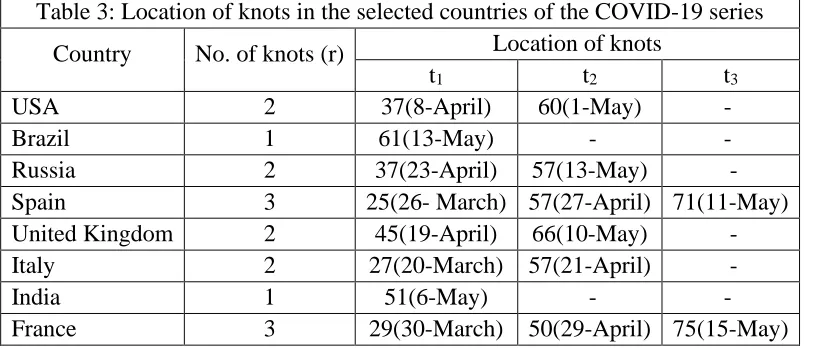
and getting the time point parallel to a maximum probability. The estimated value of the location

of knots is recorded in Table 3.

Table 3: Location of knots in the selected countries of the COVID-19 series

Country No. of knots (r) Location of knots

t1 t2 t3

USA 2 37(8-April) 60(1-May) -

Brazil 1 61(13-May) - -

Russia 2 37(23-April) 57(13-May) -

Spain 3 25(26- March) 57(27-April) 71(11-May)

United Kingdom 2 45(19-April) 66(10-May) -

Italy 2 27(20-March) 57(21-April) -

India 1 51(6-May) - -

France 3 29(30-March) 50(29-April) 75(15-May)

Table 3 shows that most of the countries have first-knot point at the early stage of the country’s

decision about shutdown/lockdown or when near to a higher number of coronavirus cases. As the

number of instances of daily coronavirus cases decline after the high peak, the second-knot point

has occurred some of the country’s series. This shows that these countries follow a downward

pattern of COVID-19 cases. In all countries, there is a significant change in the rapid decrement

of COVID cases such as Spain, France, whereas a major increment in some countries series such

as Brazil, India in the month of May, so a knot point also occurs in this month. This happens

because most of the countries give some relaxation in the lockdown that may suddenly increased

the coronavirus cases and some countries recorded control cases as observed in the previous

March and April months.

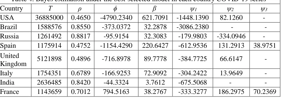
Based on Bayesian estimators, the estimated values of the best-fitted model parameters for each

country series summarizes in Table 4. Table 4 concluded that there is more variability in each

country series as all record a higher number of conformed COVID cases. The positive value of β indicates that all countries recorded a definite linear trend pattern in the complete series. The

negative of estimated coefficient of spline function shows a positive increment trend pattern

(12)

whereas the positive value of ψ describes a gradually decreased or constant pattern of confirmed cases of COVID-19.

Table 4: Bayes estimation under the best-selected model in each country COVID-19 series

Country Τ ρ ϕ β ψ1 ψ2 ψ3

USA 36885000 0.4650 -4790.2340 621.7091 -1448.1390 82.1260 -

Brazil 1588576 0.8550 -373.0372 32.2878 -3086.2380 - -

Russia 1261492 0.8817 -95.9154 32.3083 -179.9803 -334.0946 -

Spain 1175914 0.4752 -1154.4290 220.6427 -612.9536 131.2913 38.9751

United

Kingdom 5121898 0.4896 -716.8978 89.7778 -384.7725 66.6147 -

Italy 1754351 0.6789 -166.9253 72.9092 -304.2422 13.9649 -

India 2636485 0.8420 -44.3324 3.7612 -675.5068 - -

France 1143659 0.7012 794.5163 38.2767 -333.3277 186.2975 70.2369

5. Conclusion

Nowadays, COVID-19 pandemic disease is a severe challenge for the human being to survive on

earth. COVID-19 has a wide range of consequences on human life worldwide because lakhs of

people die due to coronavirus. So, there is a need to study the growth of COVID-19 cases based

on various predictive models. According to the daily reported cases, the structure of the

COVID-19 series in various countries is not linear because there are many reasons such as

lockdown, infection modes, poor health infrastructure that control or expand this disease in the

region. In this paper, we deal with a non-linear time series model using the spline function that

switches the non-linear trend component into the linear trend. It makes the analysis based on

different segments and fits the linear trend autoregressive model in each segment. Parameter

estimators and the number of knots is determined under Bayesian approach. The results

concluded that the number knots and its locations mainly depend upon the countries decision

about the controlling of the coronavirus spread using several steps such as lockdown, social

distancing, compulsory to wearing a mask, etc. These countries series are properly analyzed the

non-linear trend by using spline function when anyone correctly identified the change points in

the study.

Reference

AL-Rousan, N., & AL-Najjar, H. (2020). Data analysis of coronavirus COVID-19 epidemic in

(13)

Conrad, D. J., Bailey, B. A., Hardie, J. A., Bakke, P. S., Eagan, T. M., & Aarli, B. B. (2017).

Median regression spline modeling of longitudinal FEV1 measurements in cystic fibrosis (CF)

and chronic obstructive pulmonary disease (COPD) patients. PLoS One, 12(12), 1-13.

Eubank, R. L. (1999). Nonparametric regression and spline smoothing. CRC press.

Gondauri, D., Mikautadze, E., & Batiashvili, M. (2020). Research on COVID-19 virus spreading

statistics based on the examples of the cases from different countries. Electron Journal of

General Medicine, 17 (4), 1-4.

Hurley, D., Hussey, J., McKeown, R., & Addy, C. (2006). An evaluation of splines in linear

regression. SAS Conference Proceedings: SAS Users Group International 31(SUGI 31

Proceedings), Paper 147.

Jiang, X., Zhao, B., & Cao, J. (2020). Statistical analysis on COVID-19. Biomedical Journal of

Scientific & Technical Research, 26(2), 19716-19727.

Kass, R. E., & Raftery, A. E. (1995). Bayes factors. Journal of the American Statistical

Association, 90, 773-795.

Kumar, J., Agiwal, V., Kumar, D., & Chaturvedi, A. (2020). Bayesian unit root test for AR(1)

model with trend approximated by linear spline function. Statistics, Optimization and

Information Computing, 8(2), 425-461.

Montoril, M. H., Morettin, P. A., & Chiann, C. (2014). Spline estimation of functional

coefficient regression models for time series with correlated errors. Statistics & Probability

Letters, 92, 226-231.

Morton, R., Kang, E. L., & Henderson, B. L. (2009). Smoothing splines for trend estimation and

prediction in time series. Environmetrics: The Official Journal of the International

Environmetrics Society, 20(3), 249-259.

Osmani, F., Hajizadeh, E., & Mansouri, P. (2019). Kernel and regression spline smoothing

techniques to estimate coefficient in rates model and its application in psoriasis. Medical Journal

of the Islamic Republic of Iran, 33, 90.

Qiao, B., Chen, X., Xue, X., Luo, X., & Liu, R. (2015). The application of cubic B-spline

collocation method in impact force identification. Mechanical Systems and Signal Processing,