Vertical Ionization Energies from the Average Local Electron Energy Function

Western University Western University

Scholarship@Western

Scholarship@Western

Electronic Thesis and Dissertation Repository

9-23-2019 2:30 PM

Vertical Ionization Energies from the Average Local Electron

Vertical Ionization Energies from the Average Local Electron

Energy Function

Energy Function

Amer Marwan El-Samman

The University of Western Ontario

Supervisor

Viktor N. Staroverov

The University of Western Ontario

Graduate Program in Chemistry

A thesis submitted in partial fulfillment of the requirements for the degree in Master of Science © Amer Marwan El-Samman 2019

Follow this and additional works at: https://ir.lib.uwo.ca/etd

Part of the Numerical Analysis and Scientific Computing Commons, Other Chemistry Commons, and the Physical Chemistry Commons

Recommended Citation Recommended Citation

El-Samman, Amer Marwan, "Vertical Ionization Energies from the Average Local Electron Energy Function" (2019). Electronic Thesis and Dissertation Repository. 6633.

https://ir.lib.uwo.ca/etd/6633

This Dissertation/Thesis is brought to you for free and open access by Scholarship@Western. It has been accepted for inclusion in Electronic Thesis and Dissertation Repository by an authorized administrator of

Abstract

It is a non-intuitive but well-established fact that the first and higher vertical ionization

energies (VIE) of any N-electron system are encoded in the system’s ground-state electronic

wave function, ΨN. This makes it possible to compute VIEs of any atom or molecule from

its ground-state ΨN directly, without performing calculations on the (N−1)-electron states.

In practice, VIEs can be extracted from ΨN by using the (extended) Koopmans’ theorem or

by taking the asymptotic limit of certain wave-function-based quantities such as the ratio of

kinetic energy density to the electron density. However, whenΨN is expanded in a Gaussian

basis set, the latter method fails because the ratio diverges in ther→ ∞limit. We show that, in

such cases, the first VIE of any finite system can still be estimated by taking ther→ ∞limit

of the average local electron energy function. This function is constructed from an exact or

approximate ground-state wave function of the system and approaches a system- and

method-dependent constant in ther→ ∞ limit. For Hartree–Fock and density-functional theory, this

limit reduces to the eigenvalue of the highest-occupied molecular orbital and hence the first

VIE according to Koopmans’ theorem. We also show that, in the finite-basis approximations of

these theories, this constant will generally be more negative than the eigenvalue of the

highest-occupied molecular orbital. The results are generalized to finite-basis-set post-Hartree–Fock

theory.

Summary for Lay Audience

Consider the amount of energy it takes to kick out an electron from a molecule — the

ionization energy. The ionization energy is a measure of how tightly a molecule holds on

to its electrons. Molecules with low ionization energy tend to be more reactive as they lose

electrons easily to other molecules. Because the ionization energy explains a lot about chemical

reactivity, chemists have long tried to predict it from the quantum-mechanical model of atoms

and molecules.

The quantum-mechanical model revolves around the molecule’s wave function which

en-codes all the properties of the molecule, including its ionization energy. In fact, it turns out

that the ionization energy determines the shape of the furthest region of the wave function.

That means that just by knowing the shape of that region, quantum-chemists can predict the

ionization energy or vice versa. However, in common approximations to the wave function,

the outermost region suffers the most and predicts nonsensical ionization energies. We present

the average local electron energy (ALEE). The ALEE is calculated from the wave function but

shows more promising predictions of the ionization energy in its furthest region. In fact, we

also show that its deviation from exact ionization energy follows a certain law when the ALEE

Acknowledgements

This lab has given me the opportunity to explore the very fundamentals of chemistry. It

was a truly enjoyable intellectual journey filled with confusions and epiphanies. Thank you Dr.

Staroverov for guiding me through this journey and always believing in me. Thanks to you, I

learned how to think clearly, write precisely and to always take things one step at a time. The

skills you taught me are not just helpful for research and writing, these are principles to live by.

I want to thank my good friend and leader, Egor Ospadov, who is responsible for the

pre-liminary coding of my project and for teaching me the principles of coding, supercomputing,

researching and much more. And I also want to thank all my lab colleagues, Rongfeng Guan,

Liyuan Ye, Nick Hoffman and Egor Ospadov for always being there for me in times of need.

Lastly, my deepest gratitude goes to my family. First, for my parents, Marwan El-Samman

and Nojoud Ayoubi, who struggled very hard to raise four children, take care of me when I

was a young ill child, and bring us to Canada to give us this dream education. My whole life

I will be indebted to them. Thanks also to my siblings, Ahmad, Rand and Reem El-Samman

for always pledging their full support and believing in me. I do not know where I would be

Contents

Certificate of Examination ii

Abstract ii

Summary for lay audience iii

Acknowledgements iv

List of Figures vi

List of Tables vii

List of Abbreviations viii

1 Introduction 1

1.1 Vertical ionization energy . . . 2

1.2 Computing the VIE . . . 3

1.3 Koopmans’ theorem . . . 4

1.4 Extended Koopmans theorem . . . 9

1.5 VIE via asymptotic limits of wave-function quantities . . . 13

2 Average local electron energy 17 2.1 ALEE of the Hartree–Fock and Kohn–Sham methods . . . 17

2.2 ALEE of the post-Hartree–Fock methods . . . 20

2.3 Asymptotic limit of the average local electron energy . . . 21

2.3.1 Asymptotic limit of Kohn-Sham ALEE . . . 21

2.3.2 Asymptotic limit of Hartree–Fock ALEE . . . 22

2.3.3 Asymptotic limit of Post-Hartree–Fock ALEE . . . 23

3 Asymptotic limit of the ALEE 25 3.1 The case of Kohn–Sham ALEE . . . 25

3.2 Kohn–Sham ALEE in the basis set limit . . . 29

3.3 Hartree–Fock ALEE in the basis-set limit . . . 31

3.4 Asymptotic limit of generalized ALEE in a finite basis . . . 36

3.5 The most diffuse basis function must be in the HOMO . . . 40

3.6 Asymptotic limit of the ALEE in different directions . . . 45

3.7 Summary . . . 49

List of Figures

1.1 X-ray photoelectron spectrum of crystalline Fe2O3 . . . 1

1.2 Vertical ionization of a diatomic molecule . . . 2

1.3 Cancellation of error in the Hartree–Fock frozen-orbital VIE approximation . . . 9

1.4 The complete active space self-consistent field wave function . . . 10

1.5 τL(r)/ρ(r) for a hydrogen atom . . . 15

3.1 Kohn–Sham ALEE for the Be atom calculated using the PBEPBE functional and the cc-pVQZ basis set . . . 26

3.2 Detail of the Kohn–Sham ALEE for the Be atom using the PBEPBE functional and the cc-pVQZ basis set . . . 27

3.3 Kohn–Sham ALEE for the Be atom calculated using the PBEPBE functional and the aug-cc-pVQZ basis set . . . 28

3.4 Hartree–Fock ALEE for the Be atom calculated using the cc-pVQZ basis set . . . 32

3.5 Hartree–Fock ALEE for the Be atom calculated using the aug-cc-pVQZ basis set . . . 33

3.6 Post-Hartree–Fock ALEE for the Be CAS(4,5) system calculated using the cc-pVQZ basis set . . . 37

3.7 Detail of the post-Hartree–Fock ALEE for Be CAS(4,5) system calculated using the cc-pVQZ basis set . . . 38

3.8 Post-Hartree–Fock ALEE for Be CAS(4,5) system calculated using the aug-cc-pVQZ basis set. In this basis set the asymptotic limit of the ALEE tends to a significantly more negative value in the limit. . . 39

3.9 Hartree–Fock ALEE for CH₄using the cc-pVDZ basis set . . . 41

3.10 Hartree–Fock ALEE for CH4using the cc-pVDZ basis set modified by adding a diffuse p-type function on carbon atom . . . 43

3.11 Illustration of H₂O’s HOMO . . . 45

3.12 Contour plot of the Hartree–Fock ALEE for H2O . . . 46

3.13 Illustration of NH3’s HOMO . . . 47

List of Tables

3.1 Asymptotic limit of Kohn–Sham ALEE in finite-basis approximation . . . 31 3.2 Asymptotic limit of the Hartee–Fock ALEE in finite-basis approximation . . . 35 3.3 Asymptotic limit of post-Hartree–Fock ALEE in the finite-basis approximation . . . . 37 3.4 Asymptotic limit of the ALEE when the most diffuse basis function is almost

List of Abbreviations

VIE Vertical Ionization Energy KT Koopmans’ Theorem

EKT Extended Koopmans Theorem HOMO Highest Occupied Molecular Orbital

CASSCF Complete-Active Space Self-Consistent Field ALEE Average Local Electron Energy

Chapter 1

Introduction

Chemistry primarily deals with the structure and properties of many-electron systems. One

way to understand such systems is to take them apart, one electron at a time. This is what makes

the ionization process fundamental. Consider, for instance, the various energies required to

re-move electrons from the surface of a material. These ionization energies (measured by x-ray

photoelectron spectroscopy or energy-dispersive x-ray spectroscopy) can be used to determine

the elemental composition of that surface [1–3] (Figure 1.1). Because different elements

re-quire distinct energies to remove electrons, the spectrum can be used as a chemical fingerprint.

As an example, the peaks at specific binding energies in Figure 1.1 is characteristic of iron and

is a result of ionization from the various orbitals of the iron atom.

Even more important is the fact that the ionization energy is strongly linked to chemically

relevant concepts such as electronegativity, polarizability and atomic-shell structure [5–7].

This means that the ionization reaction is key to understanding many other chemical reactions.

There are two types of ionization reactions: adiabatic and vertical ionization. The difference

is that the former involves changes in the molecular geometry while the latter does not. The

focus of this thesis is on the vertical ionization energy which happens to be the most common

type.

1.1

Vertical ionization energy

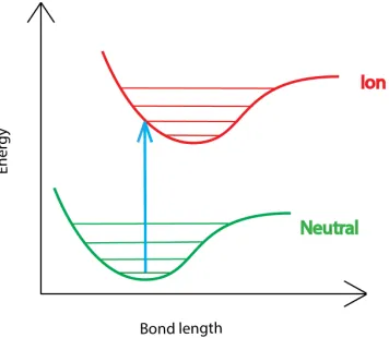
Vertical ionization is ionization which does not involve changes in the molecular geometry

(Figure 1.2)

M−→M++e− (1.1)

It is the most common type of ionization and that is because electrons, being much lighter than

the nuclei, move at a much faster rate [8–10].

The energy associated with vertical ionization is called thevertical ionization energy(VIE).

There has been much effort devoted to the accurate computation of the VIE because this

prop-erty is important for chemical exploration and because it determines the long-range behavior

of wave functions. This thesis will touch on both aspects: computing the VIE and studying the

role that the VIE plays in determining the behavior of the wave function and

wave-function-based quantities.

1.2

Computing the VIE

Several methods have been developed to obtain the VIE of a system. The most direct is

the∆SCF method, in which the VIE is computed as the difference between some ionic-state

energy and the neutral ground-state energy,

I=EN−1−EN. (1.2)

The energiesEN andEN−1are computed by solving the Schr¨odinger equation [12],

ˆ

HΨN(x1,x2,...,xN) = ENΨN(x1,x2,...,xN), (1.3)

whereΨN(x1,x2,...,xN) is the many-electron wave function,xi=(ri,si) represents the spin and

position coordinates of electroni, and the Hamiltonian operator, ˆH, is given by

ˆ

H = −1 2

N

X

i=1 ∇_i2−

N

X

i=1 nuclei

X

A=1 Z_A |ri−RA|+

N

X

i<j

1 |ri−rj|+

nuclei X

A<B

Z_AZ_B |RA−RB|

, (1.4)

whereN is the total number of electrons, ∇2_i is the Laplacian operator for theith electron and

Oppenheimer approximation [12], where nuclear and electronic wave functions are assumed to

be separable (because nuclei move at a much slower rate than electrons).

The∆SCF method requires two calculations to determine the VIE, one for theN-electron

system and one for the (N−1)-electron system. However, it has been argued [13] that as

an electron moves further and further away from an N-electron system, the N-electron wave

function should resemble the (N−1)-electron wave function, that is,

lim

|rN|→∞

ΨN_(x

1,x2,...,xN)∼ΨN−1(x1,x2,...,xN−1). (1.5)

This implies that the VIE is encoded in the N-electron wave function itself. Section 1.3 and

1.4 introduce the (extended) Koopmans’ theorems, which are standard methods of extracting

the VIE from the wave function. Then in Section 1.5 we will delve into the important role

the VIE plays in governing the long-range behavior of wave functions. In that section we

will demonstrated that the VIE may also be extracted from the long-range behavior of certain

wave-function-based quantities.

1.3

Koopmans’ theorem

Koopmans’ theorem(KT) and theextended Koopmans theorem(EKT) allow one to extract

the VIE from theN-electron wave function alone. Koopmans’ theorem only works for the

spe-cial case of Hartree–Fock wave functions, whereas the extended Koopmans theorem is

appli-cable to any approximate or exact wave function (including Hartree–Fock). But to understand

the more general case it is first important to understand the original Koopmans’ theorem for

Hartree–Fock wave functions.

The Hartree–Fock wave function is the simplest approximation to the N-electron wave

spin-orbitals also known as the Hartree–Fock Slater determinant,

Φ(x1,x2,...,xN)=

1 √

N!

N! X

i=1

(−1)pi_Pˆ

iψ1(x1)ψ2(x2)...ψN(xN)

= √1 N!

ψ1(x1) ψ2(x1) · · · ψN(x1)

ψ1(x2) ψ2(x2) · · · ψN(x2) ... ... ... ... ψ1(xN) ψ2(xN) · · · ψN(xN)

(1.6)

where ˆPiis the permutation operator,piis its parity, and each spin-orbital,ψi(x), is made up of

a spin-functionσi(which may take on a value of±1

2) and a spatial-functionφi(r),

ψi(x)=φi(r)σi. (1.7)

Finding the spin-orbitals of a system is done by using the variational principle. This principle

states that the wave function with the lowest energy is the closest to the exact ground-state

energy and exact wave function. So, finding the most accurate Hartree–Fock approximation

amounts to finding the set of spin-orbitals that give the lowest possible energy. Stated

mathe-matically, by minimizing the expectation value of ˆHfor the Hartree–Fock wave function with

respect to its spin-orbitals one can arrive at an eigenvalue equation for the minimum-energy

spin-orbitals,

ˆ

Fψi(x)=εiψi(x). (1.8)

Here ˆFis the Fock operator given by

ˆ

where

ˆ

h = −∇ 2 i

2 +v(ri) (1.10)

is the core (bare-nucleus) Hamiltonian,

ˆ J=

N

X

k=1 Z

ψk(x2)

1

r₁₂ψk(x2) dx2 (1.11)

is the Coulomb repulsion operator, and ˆK is the exchange operator whose action on a

spin-orbital is defined by

ˆ

Kψ_i(x1)= N

X

k=1 ψk(x1)

Z

ψ∗ k(x2)

1 r12

ψi(x2) dx2. (1.12)

The spin-orbitals of the Hartree–Fock wave function are the lowest-energy eigenfunctions of

the Fock operator. In terms of these spin-orbitals, the total ground-state energy of the Hartree–

Fock system is given by

EN =

N

X

i=1 h_ii+1

2

N

X

i j=1

(J_{i j}−K_{i j}), (1.13)

where

hii=

Z

ψ∗

i(x1)ˆhψi(x1) dx1 (1.14)

corresponds to the kinetic energy and nuclear attraction of an electron inψi,

J_{i j} = Z

ψ∗

is the electron-electron repulsion integral, and

K_{i j} = Z

ψ∗

i(x1) ˆKψj(x1) dx1 (1.16)

is the exchange integral.

Now using the total energy in terms of spin-orbitals, the VIE can be written as the difference

in total energies between the ground-state N-electron Hartree–Fock wave function and some

ionic-state (N−1)-electron Hartree–Fock wave function at the same geometry

I = EN−1−EN =

N−1 X

i=1 h_ii+1

2

N−1 X

i j=1

(J_{i j}−K_{i j})− N

X

k=1

h_kk+1 2

N

X

kl=1

(J_kl−K_kl). (1.17)

Since the ground and ionic states have different spin-orbitals, calculation of the VIE requires

running two Hartree–Fock calculations: for the the N- and (N−1)-electron systems (∆SCF

method). To extract the VIE from theN-electron wave function alone, an assumption has to be

made.

The assumption is that the spin-orbitals remain frozen between theN- and (N−1)-electron

systems (i.e., they do not change shape). The only difference would be that the (N−1)-electron

system has one missing spin-orbital, denotedk, because of one missing electron. Then the VIE

is written with the same spin-orbitals on either side of the subtraction in Eq. (1.17)

I = E_kN−1−EN =

N−1 X

i=1,i,k h_ii+1

2

N−1 X

i j,i,k,j,k

(J_{i j}−K_{i j})− N

X

i=1 h_ii+1

2

N

X

i j=1

(J_{i j}−K_{i j}). (1.18)

Subtracting out the common spin-orbitals in both systems leaves behind

I=−(h_kk+

N

X

i=1

which is just the eigenvalue of spin-orbitalk,

I_k=−ε_k. (1.20)

This was Koopmans’ result, a prescription for frozen-orbital VIEs within the Hartree–Fock

theory. Each occupied spin-orbital eigenvalue corresponds to one of the frozen-orbital VIEs of

the system. Thehighest occupied molecular spin–orbital (HOMO) eigenvalue corresponds to

the first VIE,

I1=−εHOMO. (1.21)

Koopmans’ theorem is the first successful attempt to seek out the ionization energy to various

(N−1)-electron states from theN-electron wave function alone. Even though the frozen-orbital

approximation is used in this method, Koopmans’ theorem gives reasonable estimates of the

experimental VIEs. For example, for an Ar atom, Koopmans’ first VIE is 0.590 E_h and the

experimental value is 0.579 E_h. For H₂O, Koopmans’ theorem predicts 0.508 E_h while the

experimental value is 0.464E_h. This is aided by the fact that the errors known in Hartree–Fock

theory and in that inherent in the frozen-orbital approximation counteract each other (see Figure

1.3) [14]. In Figure 1.3, it is illustrated that the Hartree–Fock VIE generally underestimates

the exact VIE. This means that if relaxation was accounted for, the VIE would be even further

underestimated compared to the exact.

The main limitation of Koopmans’ theorem is that it is applicable only to Hartree–Fock

wave functions. Approximations for the N-electron wave function beyond the Hartree–Fock

theory are all collectively known as post-Hartree–Fock wave functions. The extended

Koop-mans theorem(EKT) is a generalization of the original Koopmans prescription which gives the

Figure 1.3: VIE calculated through Hartree–Fock theory is generally known to be less than the exact. This means that if relaxation is accounted for, the Hartree–Fock VIE will deviate even more from exact.

1.4

Extended Koopmans theorem

Koopmans’ theorem requires taking the negative of some Hartree–Fock occupied spin-orbital

eigenvalue. This prescription does not apply to post-Hartree–Fock wave functions because

they do not have distinct sets of occupied and unoccupied spin-orbitals. Take, for example,

the full configuration interaction wave function. This wave function is constructed not just

from one antisymmetrized product of occupied spin-orbitals, but from many; all the possible

antisymmetrized products of N occupied spin-orbitals that can be constructed out of set of K

spin-orbitals (occupied and unoccupied).

ΨFCI=cHFΦHF+ X

ra

cr_aΦr_a+X

a<b r<s

crs_abΦrs_ab+ X

a<b<c r<s<t

crst_abcΦrst_abc+... (1.22)

This is done by systematically substituting the reference Hartree–Fock occupied spin-orbitals

collection of antisymmetrized products are added together to construct the full configuration

interaction wave function [12]. This can get quite expensive with system size as the

computa-tion would have to handle an astronomical number of antisymmetrized products. Thecomplete

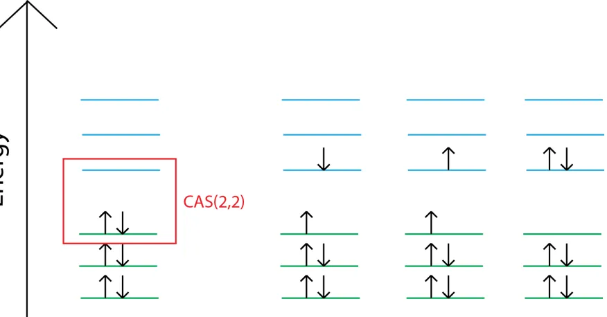
active space self-consistent field(CASSCF) method [15–17], which is one of the main

meth-ods used in this paper, allows one to choose a smaller subset of antisymmetrized products to

represent the post-Hartree–Fock wave function. An example of this is shown in Figure 1.4.

Figure 1.4: A complete active space (CAS) limits the number of configura-tions possible. It is done by choosing a subset of electrons and orbitals that are free for substitutions. The above is denoted as CAS(2,2) as the last two electrons in the last two orbitals are free to make multiple configurations.

The important thing to remember is that in post-Hartree–Fock wave functions, such as

CASSCF and full configuration interaction, there is no clear distinction between occupied and

unoccupied spin-orbitals. In fact, in the full configuration interaction wave function, all the

orbitals are partially occupied in the full set of antisymmetrized products formed. For this

While there is no inherent one-electron occupied spin-orbital in the definition of

post-Hartree–Fock wave functions, theextended Koopmans theorem(EKT) is a method to construct

this “removal orbital” from post-Hartree–Fock wave functions, such that it gives a variationally

stable (minimum of energy) (N−1)-electron wave function and corresponding VIE. The EKT

is the generalization of Koopmans’ theorem so it applies to Hartree–Fock wave functions also.

The EKT [18–21] is based on the assumption that the (N−1)-electron wave function can

be generated from theN-electron wave function using some suitably chosen removal orbital,

q_i(xN),

ΨN−1

i (x1,x2,... ,xN−1)=

Z

q_i(xN)ΨN(x1,x2,...,xN) dxN. (1.23)

Here we follow Morrison and Liu’s [19] derivation of the extended Koopmans theorem.

Equiv-alently, the assumption above can be written as

Ψ

N−1E =qˆ

Ψ

NE

, (1.24)

where

Ψ

NE _{is any wave function (exact, Hartree–Fock or post-Hartree–Fock), ˆq is a linear}

combination of annihilation operators, ˆa_i,

ˆ q=

M

X

i=1

c_iaˆ_i, (1.25)

andMis the dimension of space spanned by the spin-orbitals. Then by taking the difference in

energy between theN- and (N−1)-electron wave functions constructed according to Eq. (1.24)

we obtain the EKT matrix equation:

whereI_k is one of the VIEs,c is the vector containing the coefficients of Eq. (1.25),Gis the

generalized Fock matrix with matrix elements defined as

G_{i j}= Z

Ψ∗

(x1,x2,...,xN)ˆa†_i[ ˆHaˆj]Ψ(x1,x2,...,xN) dx1...dxN, (1.27)

andγis the one-electron reduced density matrix with matrix elements defined as

γi j = Z

Ψ∗

(x1,x2,...,xN)ˆa†_iaˆjΨ(x1,x2,...,xN) dx1...dxN. (1.28)

By solving the EKT matrix equation, one is effectively finding the removal orbital that gives a

stationary ionic state.

The EKT, Eq. (1.26), is a generalization of the Koopmans’ theorem. If a Hartree–Fock

wave function is used in Eq. (1.26), one would find that the optimal coefficients, ci, are all

zero except for a single spin-orbital. Accordingly, the VIE would correspond to the eigenvalue

of that spin-orbital. This happens because the Hartree–Fock spin-orbital already represents a

minimum energy removal-orbital of the Hartree–Fock wave function (see Section 1.3).

The EKT method is not free from problems. For example, it has been reported [19–21]

that the EKT fails for systems where the one-electron reduced density matrix is sparse. Sparse

matrices are problematic as the solution of Eq. (1.26) requires inversion of the one-electron

reduced density matrix giving

γ−1/2_Gγ−1/2_c=−I

kc. (1.29)

If the numbers in the one-electron reduced density matrix are too small, numerical inversion

becomes ill-defined and can give nonsensical VIEs.

the VIE from the N-electron wave function. However, they are not the only ones. The VIE

plays an important role in governing the long-range behavior of the wave function. So, in the

next section we show that one may theoretically be able to extract the VIE from the long-range

behavior of the wave function or certain wave-function-based quantities. However, we will

also demonstrate that this ability to extract the VIE is not possible in practical computations.

1.5

VIE via asymptotic limits of wave-function quantities

Another route to the VIE is by investigating the long-range behavior of wave function and

wave-function-based quantities. Wang and Parr [22] found that the Hartree–Fock electron

densities show approximately piecewise exponential behavior. Morrell, Parr and Levy [23]

then demonstrated that, in general, the long-range behavior of the exact electron density in the

outermost region falls off exponentially according to the equation

ρ(r)∼exp(−2p2I_minr) r→ ∞. (1.30)

The above equation means thatI_min may be extracted from the slope of lnρ(r) vs r,

lnρ(r)∼ −2p2I_minr. (1.31)

In theory, Eq. (1.31) could be used to extract the VIE from a logarithmic plot of the electron

density. However, in practical numerical calculations of the wave function, Gaussian basis

functions are used. This means that the long-range electron density decay rate is given by

where a is smallest pre-defined constant given in the basis set (as that is the one to decays

the slowest). This pre-defined constant may not be−2√2I_min and therefore, it is not possible

extract the VIE from a density expanded in a Gaussian basis set.

Another quantity that is also related to the VIE is the ratio of the kinetic energy density to

the electron density. The kinetic energy density is given by

τL(r) = −1 2[∇

2 rγ(r,r

0

)]r=r0, (1.33)

where γ(r,r0) is the one-electron reduced density matrix defined in terms of the N-electron

wave function as

γ(r,r0)=N Z

Ψ∗

(r,r2,...,rN)Ψ(r0,r2,...,rN) dr2...drN. (1.34)

Whenr0=r, theγ(r,r0) is the electron densityρ(r):

ρ(r)=γ(r,r). (1.35)

So, by evaluating the second derivative ofρ(r) to get the asymptotic kinetic energy density and

then dividing by the asymptotic electron density (Eq. 1.30) gives

lim

r→∞ τL(r)

ρ(r) =−Imin, (1.36)

revealing that the ratio theoretically approaches the first VIE of the system in ther→ ∞limit

[24].

However, in numerical approximations of the N-electron wave function where Gaussian

Substi-tution of this expression gives

τL(r) ρ(r) =−2a

2_r2_{+4ba+6a, (1.37)}

which means in ther→ ∞limit, ALEE diverges as−2a2r2 [24]. and never approaches a

con-stant. In the above evaluation, the exponential decay term cancelled out due to being common

on the numerator and denominator.

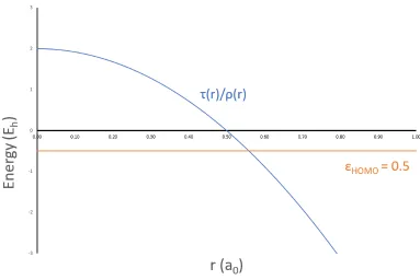
Figure 1.5 shows a graph of τL(r)/ρ(r) for the simplest system, a hydrogen atom with a

single Gaussian basis function.

Figure 1.5: τL(r)/ρ(r) for a hydrogen atom falls exponentially in the

asymptotic limit when Gaussian-type basis functions are used

It can be seen from this graph that the asymptotic limit is not the VIE of hydrogen. Therefore,

while theoretically the ratio of τL(r)/ρ(r) is supposed to approach the VIE of the system, in

In summary, both the kinetic energy density to electron density ratio and the density-tail

behavior cannot in practice give the first VIE. There is one quantity, however, which does not

show this behavior — the average local electron energy (ALEE). The ALEE approaches a

system- and method-dependent constant in ther→ ∞limit that is related to the first VIE of the

system. The focus of this thesis is on the investigating this property of the ALEE. Chapter 2

discusses the theory and background of the ALEE function and Chapter 3 examines itsr→ ∞

Chapter 2

Average local electron energy

2.1

ALEE of the Hartree–Fock and Kohn–Sham methods

Politzer and coworkers [25–29] introduced the following combination of the Hartree–Fock

occupied orbitals and orbital energies, called the average local orbital energy,

¯

εHF

(r) = 2

ρ(r)

N/2 X

i=1 εHF

i |ψ HF i (ri)|

2_,

(2.1)

where the factor of two comes from the fact that there are two spin-orbitals for each of theN/2

doubly occupied spatial orbitals of the closed-shell system. Each eigenvalue contribution is

weighed according to the square of the orbital at positionrand thus gives the average energy

coming from all the orbitals at position r. This can equivalently be called the average local

electron energy since each occupied spin-orbital carries one electron. This term is more

appro-priate for the generalized version of this quantity (see Section 2.2) as post-Hartree–Fock wave

functions do not have distinct sets of occupied and unoccupied spin-orbitals. For this reason

The ALEE is a measure of the average local eigenvalue. Since spin-orbital eigenvalues

correspond to ionization energies, the negative of the ALEE gives the average local ionization

energy at positionr,

¯

I(r)=−ε¯(r). (2.2)

Politzer and coworkers used this quantity extensively in their research on chemical reactivity,

electronegativity and polarizability of systems [5–7, 27, 30–35].

Looking at Eq. (2.1) it is not clear whether the ALEE is invariant with respect to unitary

transformation of the occupied orbitals. This is important because all quantum-mechanical

observables must have this property. The invariance is demonstrated by casting Eq. (2.1) in an

equivalent form [24, 36],

εHF

(r) = τ

HF L (r)

ρ(r) +ν(r)+νH(r)+νS(r). (2.3)

Here ν(r) is the external potential of the nuclei, τHF_L (r) is the Hartree–Fock kinetic-energy

density

τHF

L (r) = −

1 2[∇

2 rγ(r,r

0

)]r=r0, (2.4)

νS(r) is the Slater averaged exchange-charge potential

νS(r) = −

1 2ρ(r)

Z _|γ

(r,r0)|2 |r−r0_| dr

0_,

andνH(r) is the Hartree potential

νH(r) =

Z ρ

(r2) |r−r2|

dr2, (2.6)

all expressed in terms of the one-electron reduced density matrix, γ(r,r0), defined by Eq.

(1.34).

The orbital-invariant form of the ALEE proves that it is a fundamental quantum-mechanical

property and for this reason it has appeared not only in Hartree–Fock theory but also in Kohn–

Sham density functional theory. In Kohn-Sham, ALEE has a definition that is almost identical

to that of Hartree–Fock ALEE except that Kohn–Sham orbitals and orbital eigenvalues are used

¯

εKS_{(r) =} 2 ρ(r)

N/2 X

i=1 εKS

i |ψ KS i (ri)|

2_{, (2.7)}

with orbital-invariant form being

εKS

(r) = τ

KS L (r)

ρ(r) +ν(r)+νH(r)+νXC(r), (2.8)

where the first three terms on the right-hand side are the same as in the Hartree–Fock ALEE

except for the last term, which is here replaced by the exchange-correlation potentialνXC(r) of

density-functional theory.

The ALEE found relevance in both Hartree–Fock and Kohn–Sham theories. It helped

ex-plain chemically relevant concepts such as electronegativity [30, 31] and polarizability, [27, 32]

and was a good predictor of molecular reactivity sites [5–7, 33–35]. In addition to all this,

it was demonstrated that the ALEE is a fundamental ingredient for the exact formulation of

density-functional’s exchange potential [36–38]. For these reasons, it was found necessary to

2.2

ALEE of the post-Hartree–Fock methods

The ALEE was only defined for Hartree–Fock and Kohn–Sham theories until Staroverov

and Ryabinkin [24] introduced an appropriate definition applicable to post-Hartree–Fock wave

functions. The post-Hartree–Fock ALEE is defined as the diagonal part of the kernel of the

generalized Fock operator ˆGdivided by the electron density

¯

εWF_(r)= G(r,r)

ρ(r) , (2.9)

where the kernel is defined in terms of density matrices as

G(r,r0)=

−1 2∇

2 r+ν(r)

γ(r,r0)+2

Z Γ

(r,r2;r0,r2) |r−r2|

dr2. (2.10)

Since the post-Hartree–Fock ALEE only involves the diagonal elements of the above matrices,

it is written explicitly as

¯

εWF_(r)= τ WF L (r)

ρ(r) +ν(r)+νH(r)+

Z υhole

XC(r,r2) |r−r2|

dr2, (2.11)

whereυhole_XC(r,r2) is the exchange-correlation hole density. The post-Hartree–Fock ALEE was

purposely defined in the more general orbital-invariant form. But it can also be defined

specif-ically in terms of the orbitals and eigenvalues of the generalized Fock operator, f_i(r) and λi,

respectively,

¯

εWF_(r)= 2 ρ(r)

M

X

i=1

λi|fi(r)|2. (2.12)

This equation formally resembles the original definition of the Hartree–Fock ALEE, Eq. (2.1).

means that it reduces to the Hartree–Fock ALEE if a Hartree–Fock wave function is used.

This happens because the generalized Fock operator reduces to a Fock operator for Hartree–

Fock wave functions. In the next section it will be demonstrated that the theoretical r → ∞

limit for Hartree–Fock ALEE, exact density-functional ALEE, and post-Hartree–Fock ALEE

all approach exactly the first VIE of the system.

2.3

Asymptotic limit of the average local electron energy

The r → ∞ limit of the ALEE approaches a system- and method-dependent constant for

Hartree–Fock, post-Hartree–Fock and Kohn–Sham systems. This section will show this

con-stant is the first VIE for all these systems. Starting with the simplest case to analyze: the

Kohn–Sham case.

2.3.1

Asymptotic limit of Kohn-Sham ALEE

Consider first, the Kohn–Sham system which is made up of an antisymmetrized product of

Kohn–Sham spin-orbitals. These spin-orbitals have the following long-range behavior [39]:

ψi(r)∼rBiexp(−

p

−2εir) r→ ∞, (2.13)

whereB_iis some constant that is largest for the HOMO. The above equation demonstrates that

the asymptotic behavior of each Kohn–Sham spin-orbital is determined by its own eigenvalue.

Since the HOMO has the smallest eigenvalue and the largest B_i, it follows that the HOMO is

also the last orbital to decay in the Kohn–Sham system. This means that Eq (2.7) for Kohn–

Sham ALEE reduces to

lim

r→∞ε¯

KS_(r)=εKS

in the asymptotic limit. In exact density-functional theory, εKS_HOMO is the negative of the first

VIE of the system,

εKS

HOMO=−Imin. (2.15)

However, in approximate density-functional theory it would only be an approximation to the

first VIE [39].

2.3.2

Asymptotic limit of Hartree–Fock ALEE

Now let us consider the Hartree–Fock wave function which is also made up of spin-orbitals.

However, Hartree–Fock spin-orbitals have subtly different properties than those of Kohn–

Sham. In particular, the long-range behavior of a Hartree–Fock spin-orbital is, in general, a

function of all eigenvalues of the system,

ψi(r)∼ N

X

i=1

rBi_exp(−p₋₂ε

ir) r→ ∞, (2.16)

whereB_i is some constant that is largest for the HOMO [40–42]. The above equation implies

that since the HOMO has the smallest spin-orbital eigenvalue, it determines the asymptotic

behavior of all the spin-orbitals,

ψi(r)∼rBHOMO_exp(−p₋₂ε

HOMOr) (2.17)

This is a different result than that of Kohn–Sham spin-orbitals, where the asymptotic behavior

of each spin-orbital is determined by its own eigenvalue. While there is a subtle difference in

the long-range behavior between the Hartree–Fock and Kohn–Sham systems, the last orbital to

the Hartree–Fock ALEE would thus give a similar result to Kohn–Sham ALEE:

lim

r→∞ε¯

HF_(r)=εHF

HOMO. (2.18)

Here,−εHF

HOMO, according to Koopmans’ theorem equals the first VIE.

2.3.3

Asymptotic limit of Post-Hartree–Fock ALEE

Lastly, for post-Hartree–Fock wave functions, the asymptotic limit is computed using the

right-hand side of Eq. (2.11). As one electron moves away from the nuclei, the external

po-tential of the nuclei,ν(r), the exchange-correlation hole density,υhole_XC(r,r2), and the coulombic

repulsion from other electrons, νH(r), all vanish. Therefore, the only term left to analyze is τL(r)/ρ(r) in the asymptotic limit. Since it is known [23, 43, 44] that in the r → ∞ limit,

γ(r,r) (and electron density, ρ(r)) has an exponential fall-off factor given by exp(−cr) with

c= √2I_min, Eq. (2.4) gives

τWF

L (r)∼ −

1 2∇

2

rexp(−cr) r→ ∞, (2.19)

Then

lim

r→∞ε¯

WF

(r)= lim

r→∞ τWF

L (r)

ρ(r) =−Imin. (2.20)

Therefore, for post-Hartree–Fock wave functions the asymptotic limit of the ALEE approaches

the negative of the first VIE which would equal exactly the one given by EKT. Note that Eq.

(2.17) is not appropriate for the computation of the asymptotic limit of the ALEE because,

as was mentioned in section 1.4, in a Gaussian basis set, the asymptotic limit of this quantity

determined by the most diffuse basis function found on both the numerator and the

denomina-tor. Thus the basis function cancels out in the asymptotic limit and the ALEE will approach

a constant that approximates the first VIE of the system in that basis-set. This is significant

as other wave-function-based quantities diverge in a Gaussian-basis set (see section 1.4). The

next chapter of this thesis investigates the behavior of the asymptotic limit of the ALEE in a

Chapter 3

Asymptotic limit of the ALEE

The objective of this thesis is to explore the asymptotic limit of the ALEE within the Hartree–

Fock, post-Hartree–Fock and Kohn–Sham descriptions of the system. We demonstrated that

ther→ ∞limit of the ALEE theoretically approaches the first VIE at each of these levels of

theory. This section analyzes this behavior in numerical computations of the wave function

using Gaussian basis sets.

3.1

The case of Kohn–Sham ALEE

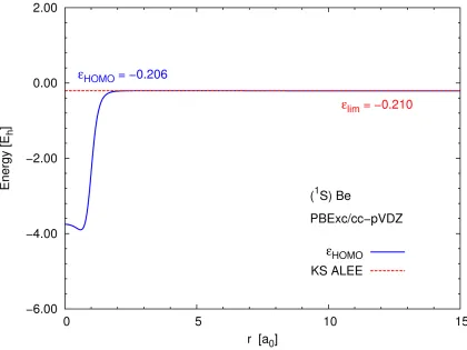
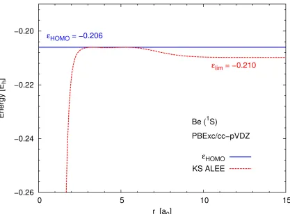
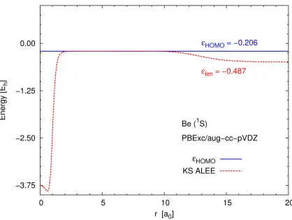
Figure 3.1 shows the asymptotic limit of the Kohn–Sham ALEE for a Be atom calculated

using the cc-pVQZ basis set. The Kohn–Sham ALEE seems to approach the eigenvalue of the

HOMO, as expected from Eq. (2.14). However, when zoomed in aroundεKS_HOMO (see Figure

3.2), it is evident that the plot of the ALEE actually tends to a slightly more negative value in the

asymptotic limit. The actual limit varies with the basis set: for instance, in the aug-cc-pVQZ

basis, the ALEE reaches an even more negative value (see Figure 3.3).

The basis-set sensitivity suggests this has to do with the finite-basis-set approximation used

in the computation of the spin-orbitals. We will show that in the finite-basis approximation, the

ALEE will give a different asymptotic value than the theoretical one. This will account for the

3.2

Kohn–Sham ALEE in the basis set limit

This section will show that spin-orbitals expressed in a finite basis give a different equation

for the asymptotic limit of the Kohn–Sham ALEE than the theoretical limit, Eq. (2.14), where

no basis set approximation is considered.

In general, the Kohn–Sham spin-orbitals cannot be solved for analytically. This is

be-cause the one-electron Kohn–Sham Hamiltonian for a spin-orbital depends on the solutions

of all other spin-orbitals in the system which are initially unknown. In practice, the Kohn–

Sham equation is solved through an iterative numerical procedure called the self-consistent

field method [12]. In this method, an initial guess for all the spin-orbitals is assumed. This

guess is constructed from a finite set of fixed chosen basis functions

ψi(r)=

M

X

j=1

cjiχj(r). (3.1)

The variational coefficients c_ji specify the contribution of basis functions χj(r) in the

spin-orbitalψi(r). Then the initial guess of spin-orbitals is used to calculate the one-electron Kohn–

Sham Hamiltonian matrix and solve the eigenvalue equation for a second set of spin-orbitals.

This process is repeated until the spin-orbitals on output is the same as on input. This is when

the solution is said to be “self-consistent.”

However, in order to get the exact spin-orbitals from the initial guess, there must be an

infi-nite number of basis functions in the spin-orbital expansion. Of course, in reality, only a fiinfi-nite

number can be used. Therefore, all solutions to the one-electron Kohn–Sham Hamiltonian will

be limited by the finite basis set. Now we are in a position to prove that due to the finiteness of

the basis set, the Kohn–Sham ALEE will generally approach a different (always more negative)

constant than the theoretical value.

orbitals are expressed using a finite set of basis functions. Thus, the finite-basis Kohn–Sham

ALEE is written as

¯

εKS_(r)= N/2

P

i=1 M

P

µ=1 M

P

ν=1 εKS

i cµicνiχµ(r)χν(r) N/2

P

i=1 M

P

µ=1 M

P

ν=1

c_µic_νiχ_µ(r)χν(r)

. (3.2)

Ther→ ∞limit of the above expression for the Kohn–Sham ALEE would depend solely on

the contributions of the most diffuse basis function,χω(r), employed in the calculation. So, in

the asymptotic limit, the above equation reduces to

aKS_lim= lim

r→∞ε¯

KS_(r)= N/2

P

i=1 εKS

i |cωi| 2

N/2 P

i=1 |c_ωi|2

, (3.3)

where c_ωi is the coefficient of the most diffuse basis function in the spin-orbital ψi(r). The

above equation for the asymptotic limit of the Kohn–Sham ALEE is notεHOMOas was derived

in section 2.3. Instead it is a linear combination of all the spin-orbital eigenvalues. This is

because the most diffuse basis function is found in all the spin-orbitals, meaning that all of

them spin-orbitals are found in the asymptotic region of the wave function. Additionally, since

the lower-lying eigenvalues are less than or equal to the HOMO energy,

εKS i ≤ε

KS

HOMO, (3.4)

the Kohn–Sham ALEE’s asymptotic limit will generally be less than the HOMO eigenvalue as

seen in Figure 3.2 and 3.3.

The constant will give exactly εKS_HOMO only when the most diffuse basis function appears

is compared in two basis sets. The basis set which has the most diffuse basis function heavily

allocated to the HOMO relative to the other orbitals will give a value much closer toεKS_HOMOin

ther→ ∞limit. The table also shows the value obtained using the finite-basis equation for the

ALEE, Eq. (3.3), to show that it gives exactly the same value as that obtained graphically.

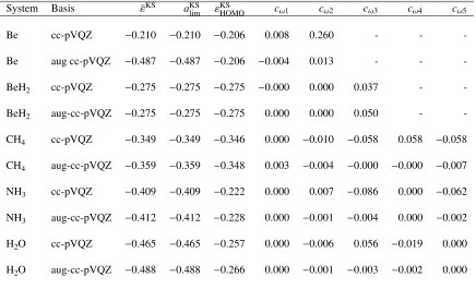
Table 3.1: The asymptotic limit of the Kohn–Sham ALEE (E_h), the prediction of Eq. 3.3 (E_h) of the ALEE, the εKS_HOMO (E_h), and coefficients of the most diffuse basis function in all the spin-orbitals. All computed using the PBEPBE functional at equilibrium geometry.

System Basis ε¯KS aKS_lim εKS_HOMO cω1 cω2 cω3 cω4 cω5

Be cc-pVQZ −0.210 −0.210 −0.206 0.008 0.260 - -

-Be aug cc-pVQZ −0.487 −0.487 −0.206 −0.004 0.013 - -

-BeH₂ cc-pVQZ −0.275 −0.275 −0.275 −0.000 0.000 0.037 -

-BeH₂ aug-cc-pVQZ −0.275 −0.275 −0.275 0.000 0.000 0.050 -

-CH₄ cc-pVQZ −0.349 −0.349 −0.346 0.000 −0.010 −0.058 0.058 −0.058

CH₄ aug-cc-pVQZ −0.359 −0.359 −0.348 0.003 −0.004 −0.000 −0.000 −0.007

NH₃ cc-pVQZ −0.409 −0.409 −0.222 0.000 0.007 −0.086 0.000 −0.062

NH₃ aug-cc-pVQZ −0.412 −0.412 −0.228 0.000 −0.001 −0.004 0.000 −0.002

H₂O cc-pVQZ −0.465 −0.465 −0.257 0.000 −0.006 0.056 −0.019 0.000

H2O aug-cc-pVQZ −0.488 −0.488 −0.266 0.000 −0.001 −0.003 −0.002 0.000

3.3

Hartree–Fock ALEE in the basis-set limit

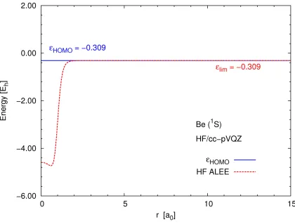
Figure 3.4 shows the ALEE for the Hartree–Fock Be atom calculated using the cc-pVQZ

basis set. In this figure, the Hartree–Fock ALEE reaches almost exactlyεHF_HOMO in ther→ ∞

limit. However, in the aug-cc-pVQZ basis set (Figure 3.5), the limit of the Hartree–Fock

ALEE gives a more negative value than εHF_HOMO. Therefore, the constant the Hartree–Fock

Figure 3.4: Hartree–Fock ALEE for Be atom calculated using the cc-pVQZ basis set. In this basis set the r → ∞ limit of the ALEE reaches

εHF

The basis-set sensitivity points again to the fact that the Hartree–Fock spin-orbitals, just

like those of Kohn–Sham, are computed using the finite-basis-set approximation. This means

that the Hartree–Fock ALEE, Eq. (2.1), when expressed explicitly in terms of basis functions

gives

¯

εHF

(r)=

N/2 P

i=1 M

P

µ=1 M

P

ν=1 εHF

i cµicνiχµ(r)χν(r) N/2

P

i=1 M

P

µ=1 M

P

ν=1

c_µic_νiχ_µ(r)χν(r)

, (3.5)

which in ther→ ∞limit gives an analogous expression for the Kohn–Sham ALEE in a finite

basis set

aHF_lim= lim

r→∞ε¯

HF_(r)= N/2

P

i=1 εHF

i |cωi| 2

N/2 P

i=1 |c_ωi|2

. (3.6)

This means that the Hartree–Fock ALEE will also in general reach a more negative constant

than εHF_HOMO in a finite basis set due to the inclusion of other spin-orbitals in the asymptotic

region. The formula above is formally similar to that of Kohn–Sham ALEE. It may seem

redundant to state almost the same formula twice, but there is good reason to do this. As

mentioned in section 2.3, Kohn–Sham and Hartree–Fock spin-orbitals have subtly different

long-range behavior. A Kohn–Sham spin-orbital’s long-range behavior is determined by its

own eigenvalue, whereas a Hartree–Fock spin-orbital’s long-range behavior is determined by

all spin-orbital eigenvalues in the system. Although the spin-orbital behavior in both theories is

governed by different laws, the Kohn–Sham and Hartree–Fock ALEEs have the same

asymp-totic limit because the HOMO happens to be the last-decaying orbital in both theories [39–42].

Another similar observation can also be made about Hartree–Fock ALEE. Only when the

limit of the Hartree–Fock ALEE give exactly εHF_HOMO. This pattern can be seen in Table 3.2,

which compares each system in two different basis sets. The basis set which has its most

diffuse function heavily allocated to the HOMO relative to the other orbitals will give a limit

of the ALEE that is much closer toεHF_HOMO. The table also shows that the value obtained using

the finite-basis equation for the Hartree–Fock ALEE, Eq. (3.6), is the same as that obtained

graphically.

Table 3.2: The asymptotic limit of the Hartree–Fock ALEE (Eh), the prediction of Eq. 3.6

(E_h) of the ALEE, the εHF_HOMO (E_h), and coefficients of the most diffuse basis function in all the spin-orbitals. All computed using the PBEPBE functional at equilibrium geometry.

System Basis ε¯HF_(E

h) aHF_lim(Eh) εHF_HOMO(Eh) cω1 cω2 cω3 cω4 cω5

Be cc-pVQZ −0.309 −0.309 −0.309 0.001 0.294 - -

-Be aug cc-pVQZ −0.487 −0.487 −0.206 −0.024 0.088 - -

-BeH2 cc-pVQZ −0.456 −0.456 −0.448 −0.000 0.034 0.000 -

-BeH₂ aug cc-pVQZ −0.447 −0.447 −0.447 0.000 0.000 0.184 -

-CH₄ cc-pVQZ −0.547 −0.547 −0.544 0.000 0.009 0.052 0.052 0.052

CH₄ aug-cc-pVQZ −0.544 −0.544 −0.543 0.000 0.000 −0.007 −0.007 −0.007

NH₃ cc-pVQZ −0.621 −0.621 −0.431 0.000 0.004 −0.067 0.000 −0.008

NH₃ aug-cc-pVQZ −0.621 −0.621 −0.429 0.000 −0.001 0.005 0.000 −0.001

H₂O cc-pVQZ −0.695 −0.695 −0.507 −0.000 0.003 0.039 −0.014 0.000

H₂O aug-cc-pVQZ −0.724 −0.724 −0.510 0.000 −0.001 −0.004 −0.001 0.000

In summary, the Hartree–Fock and Kohn–Sham ALEE approachεHOMOtheoretically.

How-ever, in the finite-basis numerical approximation, the Hartree–Fock and Kohn–Sham ALEE

approach a different constant given by Eqs. (3.3) and (3.5), respectively. This is significant as

other techniques of obtaining the VIE through asymptotic limits, such as the asymptotic limit

3.4

Asymptotic limit of generalized ALEE in a finite basis

We will now generalize the findings of the basis Hartree–Fock ALEE to the

finite-basis post-Hartree–Fock ALEE. Post-Hartree–Fock ALEE exhibits similar behavior to that of

Hartree–Fock and Kohn–Sham ALEE. Figure 3.6 and 3.7 show a beryllium CAS(4,5) system

computed using the cc-pVQZ basis set. While in Figure 3.6 it seems as if the post-Hartree–

Fock ALEE reaches exactly the first VIE, when enlarged (Figure 3.7), it shows there is a slight

deviation. And this deviation is again basis-set sensitive (Figure 3.8). In Figure 3.8, the−Imin

significantly deviates from exact in the aug-cc-pVQZ basis set.

CASSCF wave functions and many other post-Hartree–Fock wave functions also rely on

the use of a basis set of functions. Post-Hartree–Fock ALEE is written in a finite basis set as

¯

εWF

(r)= PN/2

i j=1

PM

µ=1

PM

ν=1cµicνjGi jχµ(r)χν(r) PN/2

i j=1

PM

µ=1

PM

ν=1cµicνjPi jχµ(r)χν(r)

. (3.7)

Since the r→ ∞ limit is given by the most diffuse basis function, χω(r), the above equation

becomes

aWF_lim = lim

r→∞ε¯

WF_(r)= PN/2

i j=1cωiGi jcωj PN/2

i j=1cωiPi jcωj

(3.8)

Table 3.3 shows how the equation above predicts the constant that will be reached in the

Table 3.3: The asymptotic limit of the post-Hartree–Fock ALEE (E_h) and the prediction of Eq. 3.8 (E_h). All computed using the cc-pVQZ basis set at equilibrium geometry.

System Active Space aWF

lim (Eh) ε¯ WF _(E

h) Experimental (Eh) [11]

He (2,10) −0.901 −0.901 −0.903

Be (4,5) −0.359 −0.359 −0.342

H₂ (2,10) −0.611 −0.611 −0.567

LiH (4,6) −0.688 −0.688 −0.300

H₂O (8,10) −0.325 −0.325 −0.464

NH₃ (8,14) −0.663 −0.663 −0.368

We have shown how to calculate the asymptotic limit of the ALEE function in the

finite-basis approximation of all theories (Hartree–Fock, Kohn–Sham and post–Hartree-Fock). In

general, the ALEE does not necessarily reach the theoretical value of−I_min but approximates

depending on the coefficients of the most diffuse basis function. Next we will show how to

construct a basis such that it gives exactly−I_min.

3.5

The most diffuse basis function must be in the HOMO

We have shown that the r → ∞ limit of the ALEE approaches a system- and

method-dependent constant. Furthermore, for Hartree–Fock and Kohn–Sham systems, this constant

depends on the basis set and generally has a more negative value thanεHOMO. Now we show

that it is possible to construct a basis that meets a condition which will giveεHOMOaccurately.

The finite-basis equation for the asymptotic limit of the Hartree–Fock and Kohn–Sham

ALEE, Eqs. (3.3) and (3.5) both reduce toεHOMO if the coefficients of the most diffuse basis

functions are zero for all orbitals except the HOMO. This condition is met approximately if

a basis set is constructed with a sufficiently diffuse basis function such that it will be almost

exclusively in the HOMO expansion.

For instance, consider the methane molecule computed at the Hartree–Fock level of theory

using the cc-pVDZ basis set (Figure 3.9). The constant reached by the ALEE is more negative

thanεHOMO. That is because in this basis set, hydrogen’s second s-type function is the most

cc-pVDZ basis set for the H atom

Exponent Contraction Coefficient

S

1.301000D+01 1.968500D-02

1.962000D+00 1.379770D-01

4.446000D-01 4.781480D-01

1.220000D-01 5.012400D-01

S

1.220000D-01 1.000000D+00

P

7.270000D-01 1.0000000

Figure 3.9: Hartree–Fock ALEE for CH₄ using the cc-pVDZ basis set. The basis set exponents of hydrogen are shown above the graph. The most-diffuse basis function is being used in multiple spin-orbitals thus the ALEE reaches a more negative value thanεHOMO in the asymptotic limit. The

If an additional diffuse p-type basis function, from the aug-cc-pVDZ basis, is added to the

carbon atom in methane, then the asymptotic limit of the ALEE reaches exactlyεHOMO(Figure

3.10). This is because the additional diffuse function on carbon is not used by any orbitals other

than the triply degenerate HOMO of methane.

cc-pVDZ basis set for the C atom with an extra p-type function

Exponent Contraction Coefficient

S 6.665000D+03 6.920000D-04 1.000000D+03 5.329000D-03 2.280000D+02 2.707700D-02 6.471000D+01 1.017180D-01 2.106000D+01 2.747400D-01 7.495000D+00 4.485640D-01 2.797000D+00 2.850740D-01 5.215000D-01 1.520400D-02 1.596000D-01 -3.191000D-03 S 6.665000D+03 -1.460000D-04 1.000000D+03 -1.154000D-03 2.280000D+02 -5.725000D-03 6.471000D+01 -2.331200D-02 2.106000D+01 -6.395500D-02 7.495000D+00 -1.499810D-01 2.797000D+00 -1.272620D-01 5.215000D-01 5.445290D-01 1.596000D-01 5.804960D-01 S 1.596000D-01 1.000000D+00

P 4 1.00

9.439000D+00 3.810900D-02 2.002000D+00 2.094800D-01 5.456000D-01 5.085570D-01 1.517000D-01 4.688420D-01 P 1.517000D-01 1.0000000

P 1 1.00

4.041000D-01 1.0000000

D

Figure 3.10: Hartree-Fock ALEE for CH₄ using the cc-pVDZ basis set modified by adding a p-type basis function on the carbon atom. This func-tion is used only in the triply degenerate HOMO and therefore give the asymptotic limit as exactlyεHOMO. The coefficients of the most diffuse

Therefore, it is possible to construct a basis in which the ALEE gives exactlyεHOMO, but

this basis must adhere to the condition that the most diffuse basis function is used almost

exclusively in the HOMO. Table 3.4 shows a list of other systems where an augmented basis

(from aug-cc-pVDZ basis set) was diffuse enough to give exactlyεHOMOor−Imin.

Table 3.4: Asymptotic ALEE limits computed using the cc-pVDZ basis and the same basis augmented with an additional diffuse funciton (cc-pVDZ*), in brackets is the added diffuse basis function exponent and angular momentum.

System Wave Function cc-pVDZ cc-pVDZ* −Imin Experimental [11]

CH₄ Hartree–Fock −0.554 −0.525 (p: 0.040) −0.525 0.463 NH₃ Hartree–Fock −0.445 −0.343 (p: 0.056) −0.343 0.370 CH₄ CAS(8,8) −0.656 −0.525 (p: 0.040) −0.525 0.463 H₂O CAS(8,10) −1.362 −0.515 (p: 0.069) −0.515 0.464 NH₃ CAS(8,14) −1.244 −0.403 (p: 0.056) −0.403 0.370 HF CAS(8,9) −1.052 −0.604 (p: 0.085) −0.604 0.589

Thus, the asymptotic limit of the ALEE reveals an important difference between exact

and finite-basis wave function solutions. In exact Hartree–Fock and Kohn–Sham theory, the

HOMO is the slowest decaying orbital and it determines the asymptotic decay of the electron

density. For finite-basis wave functions, the rule that the HOMO determines the asymptotic

decay is violated because the most diffuse basis function is found in all spin-orbitals. In this

sense, all of the spin-orbitals determine the behavior of the asymptotic region of a finite-basis

wave function. The asymptotic limit of the ALEE will give εHOMO only when the

finite-basis wave function adheres to the condition that the last decaying orbital is the HOMO. This

happens precisely when the coefficients of the most-diffuse basis function is zero for all orbitals

except for the HOMO.

It is important to note that the asymptotic limit of the ALEE must be taken in a direction

that is not in the nodal plane of the HOMO to getεHOMO. For example, for H2O in the tables

above, the asymptotic limit was always evaluated in the x-axis to avoid theyz HOMO nodal

3.6

Asymptotic limit of the ALEE in different directions

In general, the asymptotic behavior of the electron density decay is non-uniform. The

pre-viously mentioned asymptotic behavior, r2bexp(−2√−2εHOMOr), is true for all directions of

the system except in a nodal plane of the HOMO. In a nodal plane the last orbital to decay is

some lower-lying orbital, HOMO−1 (assuming the HOMO−1 does not have the same nodal

place). This means that in that direction the asymptotic behavior of electron density is given

asr2bexp(−2√−2εHOMO-1r) [45, 46]. The asymptotic limit of the ALEE should be consistent

with this behavior and giveεHOMO-1 in the directions of nodal axis.

Consider, for example, the H₂O molecule which has ayznodal plane in its HOMO.

Figure 3.11: Illustration of H₂O’s HOMO

Due to the yz nodal plane it is expected that the asymptotic limit of the ALEE along the x

-axis will be εHOMO and along they- and z-axis it will beεHOMO−1. The contour plot shown

in Figure 3.12 for xy plane confirms this behavior. Along the x-axis, the ALEE approaches

The same is observed for NH₃where there is anxynodal plane (Figure 3.13).

Figure 3.13: Illustration of NH₃’s HOMO

Here, it is expected that the asymptotic limit of the ALEE along thez-axis will giveεHOMOand

along thex- andy-axis (due to thexynodal plane) will giveεHOMO−1. The contour plot shown

Figure 3.12 for theyz plane confirms this behavior. Along thez-axis, the asymptotic limit of

the ALEE approachesεHOMO (−0.419 Eh) of the system while along they-axis it approaches

εHOMO-1(−0.616Eh) due to theyznodal plane.

These results imply that the ALEE gives information about which orbital dominates the

asymptotic region. It confirms the fact that while in most directions the last decaying orbital

is usually the HOMO, in the nodal plane of the HOMO, the asymptotic behavior is dominated

by some lower-lying orbital. In this way, the asymptotic limit of the ALEE mimics the outer

3.7

Summary

The ALEE is a quantity derived from the ground-state N-electron wave function of the

system. For Hartree–Fock and Kohn–Sham systems, the ALEE theoretically approaches the

eigenvalue of the HOMO in ther→ ∞ limit. However, if the spin-orbitals are computed

us-ing the finite-basis approximation, the asymptotic limit of the Hartree–Fock and Kohn–Sham

ALEE will be a linear combination of all the occupied-orbital eigenvalues. For finite-basis

post-Hartree–Fock ALEE, the asymptotic limit is also determined by the most diffuse basis

function’s coefficients as given by Eq. (3.7).

Compared to many other wave-function-based quantities, the ALEE has the advantage that

it asymptotically approaches a constant instead of diverging in ther→ ∞limit. This constant

is exactly or approximately the first VIE. In exact Hartree–Fock and Kohn–Sham theory, the

HOMO is the slowest-decaying orbital and it determines the asymptotic decay of the electron

density, thus the ALEE would giveεHOMO. For finite-basis wave functions, that rule is violated

because the most diffuse basis function is found in all orbitals. In other words, all the

spin-orbitals determine the asymptotic decay of the system and the ALEE gives a linear combination

of eigenvalues for the asymptotic limit. Therefore, in order for a finite-basis wave function to

obey the rule that the HOMO decays last, the HOMO must have the most diffuse basis function

to itself. If this condition is met, the asymptotic limit of the ALEE will almost exactly the first

Bibliography

[1] K. Siegbahn and K. Edvarson. β-Ray spectroscopy in the precision range of 1:105.Nucl. Phys.1,8 (1956).

[2] D. W. Turner and M. I. Al Jobory. Determination of ionization potentials by photoelectron energy measurement.J. Chem. Phys.37, 3007 (1962).

[3] J. Goldestein. Scanning Electron Microscopy and X-ray Microanalysis. Kluwer Aca-demic/Plenum: London, New York; 2003.

[4] T. Yamashita and P. Hayes. Analysis of XPS of Fe2+ and Fe3+ ions in oxide materials. Appl. Surf. Sci.254, 8 (2008).

[5] J. S. Murray, T. Brinck and P. Politzer, in Theoretical Organic Chemistry, edited by C. P´ark´anyi. Elsevier, Amsterdam, 1996, pp. 189-202.

[6] P. Politzer and J. S. Murray, inTheoretical Aspects of Chemical Reactivity, edited by A. Toro-Labb´e. Elsevier, Amsterdam, 2007, pp. 119-137.

[7] P. Politzer, J. S. Murray and F. A. Bulat. Average local ionization energy: A review. J. Mol. Model.16, 1731 (2010).

[8] J. Franck. Elementary processes of photochemical reactions. J. Chem. Soc. Faraday Trans.21, 536 (1926).

[9] E. Condon. A theory of intensity distribution in band systems.Phys. Rev.28, 1182 (1926).

[10] E. Condon. Nuclear motions associated with electron transitions in diatomic molecules. Phys. Rev.32, 858 (1928).

[11] Notes on ionization energies. National Institute of Standards and Technology. https://cccbdb.nist.gov/adiabatic.asp (accessed April 09, 2009).

[12] A. Szabo and N.S. Ostlund, inModern Quantum Chemistry. (Dover Publications, New York, 1996), pp. 39-107.

[14] N. Heinrich, W. Koch and G. Frenking. On the use of Koopmans’ theorem to estimate negative electron affinities.Chem. Phys. Lett.124, 17 (1986).

[15] P. E. M. Siegbahn, A. Heiberg, B. O. Roos and B. Levy. A comparison of the super-CI and the Newton-Raphson scheme in the complete active space SCF method.Phys. Scr. 21, 323 (1980).

[16] B. O. Roos, P. R. Taylor and P. E. M. Siegbahn. A complete active space SCF method (CASSCF) using a density matrix formulated super-CI approach.J. Chem. Phys.48, 157 (1980).

[17] P. E. M. Siegbahn, J. Alml¨of, A. Heiberg and B. O. Roos. The complete active space SCF (CASSCF) method in a Newton-Raphson formulation with application to the HNO molecule.J. Chem. Phys74, 2384 (1981).

[18] O. W. Day, W. Smith and C. Garrod. Extension of Koopmans’ theorem. I. Derivation.Int. J. Quantum Chem.8, 501 (1974).

[19] R. C. Morrison and G. Liu. Extended Koopmans’ theorem: Approximate ionization en-ergies from MCSCF wave functions.J. Comput. Chem.13, 1004 (1992).

[20] M. Ernzerhof. Validity of extended Koopmans’ theorem.J. Chem. Theory Comput.5, 793 (2009).

[21] R. C. Morrison, C. M. Dixon and J. R. Mizell Jr. Examination of the limits of accuracy of the extended Koopmans’ theorem ionization potentials into excited states of ions LiH, He₂and Li₂· Int. J. Quantum Chem.52, 309 (1994).

[22] W. Wang and R.G. Parr. Statistical atomic models with piecewise exponentially decaying electron densities.Phys. Rev. A16, 891 (1977).

[23] M. M. Morell, R. G. Parr and M. Levy. Calculation of ionization potentials from density matrices and natural functions and the long-range behavior of natural orbitals and electron density.J. Chem. Phys.62, 549 (1975).

[24] V. N. Staroverov and I. G. Ryabinkin. The average local electron energy generalized to correlated wave functions.J. Chem. Phys.141, 084197 (2014).

[25] P. Sjoberg, J. S. Murray, T. Brinck and P. Politzer. Average local ionization energies on the molecular surfaces of aromatic systems as guides to molecular reactivity.Can. J. Chem. 68, 1440 (1990).

[26] J. S. Murray, J. M. Seminario, P. Politzer and P. Sjoberg. Average local ionization energies computed on the surfaces of some strained molecules. Int. J. Quantum Chem. 24, 645 (1990).