Feature Based Calibration of a Network of Kinect Sensors

(1)

Scholarship@Western

Electronic Thesis and Dissertation Repository

1-16-2018 11:00 AM

Feature Based Calibration of a Network of Kinect Sensors

Xiaoyang Li

The University of Western Ontario

Supervisor

Steven Beauchemin

The University of Western Ontario Co-Supervisor Michael Bauer

The University of Western Ontario Graduate Program in Computer Science

A thesis submitted in partial fulfillment of the requirements for the degree in Master of Science © Xiaoyang Li 2018

Follow this and additional works at: https://ir.lib.uwo.ca/etd

Part of the Artificial Intelligence and Robotics Commons

Recommended Citation Recommended Citation

Li, Xiaoyang, "Feature Based Calibration of a Network of Kinect Sensors" (2018). Electronic Thesis and Dissertation Repository. 5180.

https://ir.lib.uwo.ca/etd/5180

This Dissertation/Thesis is brought to you for free and open access by Scholarship@Western. It has been accepted for inclusion in Electronic Thesis and Dissertation Repository by an authorized administrator of

(2)

i

The availability of affordable depth sensors in conjunction with common RGB cameras, such

as the Microsoft Kinect, can provide robots with a complete and instantaneous representation

of the current surrounding environment. However, in the problem of calibrating multiple

camera systems, traditional methods bear some drawbacks, such as requiring human

intervention. In this thesis, we propose an automatic and reliable calibration framework that

can easily estimate the extrinsic parameters of a Kinect sensor network. Our framework

includes feature extraction, Random Sample Consensus and camera pose estimation from

high accuracy correspondences. We also implement a robustness analysis of position

estimation algorithms. The result shows that our system could provide precise data under

certain amount noise.

Keywords

(3)

ii

Acknowledgments

Foremost, I would like to express my sincere gratitude to my advisors Prof. Steven

Beauchemin and Prof. Michael Bauer for their continuous support of my Master study and

thesis, for their patience, motivation, enthusiasm, and immense knowledge. The door to Prof.

Beauchemin’s office was always open whenever I ran into a trouble spot or had a question

about my research or writing. I could not have imagined having a better advisor and mentor

for my Master study.

Besides my advisors, I would like to thank the rest of my thesis committee: Prof. John

Barron, Prof. Kostas Kontogiannis, and Prof. Ken Mclsaac, for their encouragement,

insightful comments, and hard questions.

Last but not the least, I would like to thank my family: my parents Gan Li and Guixiang Li,

for giving birth to me in the first place and supporting me spiritually throughout my life. This

(4)

iii

List of Tables

Table 1. Comparative Specifications of Kinect v1 and Kinect v2. ... 4

Table 2 Comparison of results from different camera pose estimation algorithms ... 54

Table 3 Comparative results from different camera pose estimation algorithms ... 57

Table 4 Synthetic Data ... 59

(8)

vii

List of Figures

Figure 1.1. Hardware configuration of Kinect v2. ... 3

Figure 1.2. Illustration of Kinect depth measurement. ... 4

Figure 3.1 Flow chart r the whole system ... 12

Figure 3.2 Stereo cameras projection. ... 13

Figure 3.3 Projection between different coordinate systems ... 15

Figure 3.4 A pinhole camera model. ... 17

Figure 3.5 Barrel Distortion and Pincushion Distortion ... 19

Figure 3.6 Points correspondence geometry (a) ... 22

Figure 3.7 Points correspondence geometry (b) ... 22

Figure 3.8 Illustration of Epipolar geometry ... 23

Figure 3.9 Epipolar constraint... 26

Figure 3.10 Input image applied with different Gaussian kernel... 28

Figure 3.11 SIFT key point descriptor ... 30

Figure 3.12 Differences between SIFT (left side) and SURF (right side) when constructing a scale space. ... 32

Figure 3.13 Orientation assignment of SURF... 33

(9)

viii

Figure 3.15 Four solution form decompose Essential Matrix.. ... 40

Figure 3.16 Re-center dataset ... 44

Figure 5.1 RGB-D image structure. ... 51

Figure 5.2 Case 1: Feature Points.. ... 53

Figure 5.3 Case 1: Correspondences.. ... 54

Figure 5.4 Case 2: Feature Points ... 56

Figure 5.5 Case 2: Correspondences ... 56

Figure 5.6 Gaussian Distribution with different values for sigma ... 60

Figure 5.7 Comparative offsets of R for sigma∈ [0,1] ... 61

Figure 5.8 Comparative offsets of T for sigma∈ [0,1] ... 61

Figure 5.9 Comparative offsets of R for sigma∈ [0,0.7] ... 62

Figure 5.10 Comparable offsets of T for sigma∈ [0,0.7] ... 62

Figure 6.1 The reflection problem with a transparent glass... 65

(10)

Chapter 1

1

Introduction

1.1 Overview

The robotics industry has been developing rapidly in the past few years. Typical robotic

tasks, like simultaneous localization and mapping (SLAM), navigation, object

recognition and many others, greatly benefit from having color and depth information

fused together. Traditional high-cost 3D profiling cameras often result in lengthy

acquisition and slow processing of massive amounts of information. With the invention

of the low-cost Microsoft Kinect sensor, high-resolution depth and visual (RGB) sensing

has created many opportunities for multimedia computing. Our objective is to design and

implement a system for calibrating multiple Kinect sensors in different views.

1.2 Kinect Mechanism

Kinect contains a normal RGB camera, an Infrared Sensor and a four-microphone array.

Combining these devices, the Kinect is able to provide RGB images, depth images and

audio signals simultaneously, which encourages varied applications in different fields,

such as image signal synchronization, human 3-D motion capture, human face

(11)

Kinect Sensing Hardware

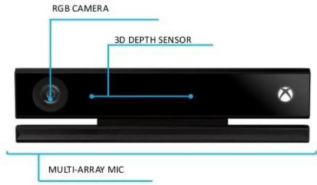
Kinect is a composite device consisting of a near-infrared laser pattern projector, an IR

camera and a color (RGB) camera; Figure 1.1 shows the arrangement of the sensors on a

Kinect. The laser pattern projector and the IR camera are used as a stereo pair to capture

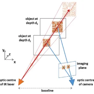
depth information in 3D space. The IR projector casts an IR speckle dot pattern into the

3D scene while the IR camera captures the reﬂected IR speckles. Due to the uniqueness

of each projected dot, the depth of a point can be captured by relative left-right translation

of the dot pattern. This translation is dependent on the distance of the object to the

camera-projector plane. Such a procedure is illustrated in Figure 1.2. [1]

Each component of the Kinect hardware is described below.

1) RGB Camera: It delivers three basic color components of the video. The camera

operates at 30 Hz, and can offer images at 1920×1080 pixels with 8-bit per channel. The

angular field of view (FOV) is 84.1° horizontally and 54.8° vertically.

2) 3-D Depth Sensor: It consists of an IR laser projector and an IR camera. Together, the

depth image is constructed by triangulation from the stereo pair. The sensor has a

practical ranging limit of 0.5 m−8.0 m distance, and outputs video at 30 frames/s with the

resolution of 512×424 pixels. The angular field of view (FOV) is 70.6° horizontally and

60.0° vertically.

Table 1 also provides comparative specifications of the Kinect v2, which is used in this

(12)

(13)

Figure 1.2. Illustration of Kinect depth measurement. IR camera could sense the

depth by the unique project pattern.

Table 1. Comparative Specifications of Kinect v1 and Kinect v2.

Kinect v1 Kinect v2

Resolution of RGB image 640 × 480(pixel) 1920 × 1080(pixel)

Resolution of IR image 320 × 240(pixel) 512 × 424(pixel)

Field view of RGB image 62° × 48.6° 84.1° × 53.8°

(14)

Maximum skeletal tracking 2 6

Method of depth measurement Lighting coding Time of Flight

Working range 0.8m~3.5m 0.5m~8.0m

1.3 Problem and Issues

Multiple-camera systems have become increasingly prevalent in robotics and computer

vision research. One of the most important tasks is how to combine the visual

information in those cameras. This problem, in general, can be interpreted as a

mathematical problem. Given two cameras, each with their own 3D coordinate system,

they obtain information of the same scene from different views. There should be a rigid

transformation between the two camera coordinates. Specifically, in 3D space, this

transformation is determined by a rotation matrix 𝑅 and a transit vector 𝒕⃗.

This problem can be stated as follows:

Assume that we have two calibrated cameras 𝐶𝑙 and 𝐶𝑟, such that the intrinsic matrices

are 𝐾_𝑙 and 𝐾_𝑟. However, the absolute positions expressed in a world coordinate system

𝑂_𝑤 between them are unknown. By giving the input RGB + Depth (RGB-D) images of

the same scene from those two cameras, can we design a system that can automatically

(15)

1.4 Thesis Contribution

This thesis presents and evaluates a framework that integrates RGB-D data capture,

feature points selection, correspondence optimization and camera pose reconstruction

into one application. The thesis also includes a robustness analysis of the approach which

demonstrates that the system is resistant to noisy data and provides precise estimation.

Besides, this thesis is the first one to introduce 3D eight-points algorithm and numerically

compare those three pose estimation algorithms.

1.5 Thesis Contents

This thesis is organized as follows:

Chapter 2 briefly describes the traditional methods of camera calibration as well as

previous work on 3D sensor calibration and address the deficiency and constraints of

each algorithm. Chapter 3 is the core of this thesis which explained in detail each stage of

the processing within the system. With respect to feature detection and correspondence

selection, we rely on the work of Lowe [2][3] and Bay and Herbert [4]. We also

leverage the camera pose estimation algorithms proposed by Lepetit [5] and Hartley [6].

In Chapter 4, the methodology that is used to build the complete system is presented and

the sets of experiments are described. The results presented in Chapter 5 illustrate the

effectiveness of the system and demonstrate its robustness to noise. Finally, Chapter 6

lists some areas of future work for potentially improving the system and proposes new

(16)

Chapter 2

2

Related Work

Camera calibration, in general, is the process of estimating the parameters of a pinhole

camera model approximating the camera that produced a given photograph or video. The

extrinsic calibration of a camera from independent pairwise correspondences with

multiple views is essentially the problem of estimating the camera positions between

non-central cameras.

Many calibration methods have been proposed to do the calibration work using a

calibration object with known world coordinates. One possible way is to use a calibration

object, which consists of several easily detectable non-coplanar feature points with

known relative 3D positions, such as a checkerboard pattern [7], [8], [9]. Corresponding

points between 3D world points and image points could be accomplished by fixing the

world coordinate system in the calibration object. Then, by optimizing the mapping from

picture coordinates system to corresponding 3D world coordinates, both intrinsic and

extrinsic parameters could then be estimated. This optimization problem could be solved

linearly if 17 correspondences are given [10]. Apart from the time complexity, 6 pairs of

correspondences, at a minimum, are also able to be used to find an acceptable estimation

[11]. However, this 6-pairs correspondence method cannot output reliable results for

some particular situations, for example, if one of the generalized views is a pin-hole. For

(17)

stereo rigs, Vasconcelos et al. propose a non-minimal solution using 10 correspondences

[12].

To conclude, these kinds of algorithms can solve the problem for calibrating a single

camera efficiently. However, when it comes to a camera network, which contains

multiple cameras, it is tedious and cumbersome to calibrate all the cameras

simultaneously using these reference objects, as it is often extremely difficult to make all

the points on the calibration object simultaneously visible in all views. Moreover,

designing highly accurate tailor-made calibration patterns are often difficult and

expensive.

Another option [13], [14] is to observe the object through planar mirror reﬂections in

order to handle situations of little or no overlap in the focal views. They overcome the

need for all cameras to have overlapping direct views by allowing them to see the object

through a mirror. They first adopt standard calibration methods to find the internal and

external parameters of a set of mirrored cameras poses and then estimate the external

parameters of the real cameras from their mirrored poses by formulating constraints

between them. However, those calibration procedures are explicit, in the sense that they

require substantial human intervention, and are meant to be carried out as an initial

off-line step before starting to operate the network of cameras.

People have also turned to 3D sensors, which offer depth information in more convincing

and precise ways. An important task for multiple cameras is the calibration for 3D

(18)

Auvinet et al. [15] proposed a method for calibrating multiple depth cameras by using

only depth information. Their algorithm is based on plane intersections and the Network

Time Protocol for data synchronization. The calibration achieves good results even if the

depth error of the sensor is 10 mm. A drawback of their implementation is that they have

to manually select the plane corners and, above all, they only deal with depth sensors,

thus avoiding the possibility to add the color information to the fused data.

Another approach to solve the calibration problem is the one proposed by Le and

Ng [16]: they jointly calibrate groups of sensors. Each group is composed by a set of

sensors that can provide a 3D representation of the world. They first calibrate the

intrinsic parameters of the sensors individually, then they calibrate the extrinsic

parameters of each group and the extrinsic parameters of each group with respect to all

the others. In the end, they refine the calibration parameters of the entire system in one

optimization step. Their experiments show that this method not only reduces the

calibration error, but also requires little human intervention.

In 2010, the Kinect for Xbox 360 sensor was introduced by Microsoft as an affordable

and real-time source for RGB-D data, which was dedicated to gesture detection and

recognition in a game controller. Due to its acquisition speed, many researchers have

recognized the potential of the Kinect’s RGB-D imaging technology, which gives a

significant rise to this field.

In order to merge data collected from different Kinect sensors, various approaches have

been proposed for simultaneous calibration of Kinect’s sensors. Burrus [17] proposes to

(19)

selection of the four corners of a checkerboard for calibrating the depth sensor. Zhang et

al. [18] propose a semi-automatic method. They automatically sample the planar target to

collect the points for calibration of depth sensor and then manually select corresponding

points between color and depth images. Combing them together, the extrinsic relationship

within a single Kinect sensor is established. Gaffney [19] describes a technique to

calibrate the depth sensor by using 3D printouts of cuboids to generate different levels in

depth images. However, after that it requires an elaborate process to construct the target.

To avoid the need for blocking the projector when calibrating, Berger et al. use a

checkerboard where black boxes are replaced with mirroring aluminum foil [20].

In conclusion, traditional methods fail to use depth information effectively which makes

them unable to determine the distance in the real world. A number of the previous 3D

sensor calibrating algorithms require human intervention and thus are tedious and

complex when calibration of multiple cameras is needed. This thesis provides a system

that can not only determine camera poses with a high precision but it is also robust to

noisy data. More importantly, it is an automatic system that requires no human

(20)

Chapter 3

3

System Description

In this Chapter, we present each component of our system in chronological order. We

introduce the theory of RGB-D image formation, depth information, pinhole camera

models and four coordinate systems. Following this, the problem of calibrating the

camera system is proposed. This part contains the definition of intrinsic and extrinsic

camera parameters and discusses the phenomenon of camera lens distortion. In order to

introduce the Essential and Fundamental Matrices, the theory of Epipolar Geometry is

also discussed.

We then discuss some common computer vison tasks such as, feature detection and

matching. Two scale-invariant feature detection algorithms, SIFT and SURF, are

presented. We also discuss a robust stochastic method (RANSAC) commonly used to

match features from source images.

Three methods of estimating camera pose from correspondences are presented. These are:

the Eight-Point algorithm (uses 2D correspondences), Perspective-n-Point (uses 3D-2D

correspondences), and 3D Point Registration (uses 3D correspondences). The system is

(21)

Figure 3.1 Flow chart r the whole system

3.1 Stereo Vision Theory

Stereo vision refers to the process of extracting 3D information from two (or more) 2D

views of a scene. In this Section, common knowledge is discussed such as disparity and

depth. In addition, the pinhole camera model as well as different coordinate systems are

introduced in order to discuss stereo vison effectively.

Disparity and Depth

Human eyes are horizontally separated by about 50–75 mm, depending on each

individual. Thus, each eye has a slightly different view of the world around. The term

binocular disparity refers to geometric measurements related to the estimation of scene

depth. In computer vision, binocular disparity is calculated from stereo images taken

from a set of stereo cameras. The variable distance between these cameras, called the

(22)

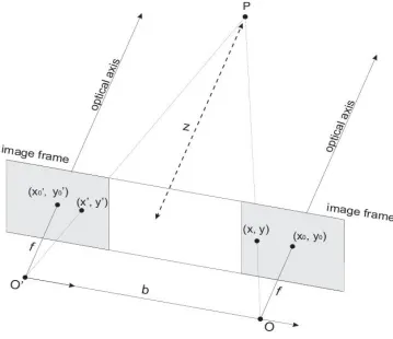
[21]. Figure 3.2 shows one point in the real world projected onto two image planes by

two cameras in different positions.

Figure 3.2 Stereo cameras projection. The quantity b refers to baseline, and (𝒙 − 𝒙′₎

is disparity.

Disparity can be used in the extraction of information from stereo images. One case that

disparity is most useful is for 3D depth estimation. Disparity and distance from the

cameras are inversely related. As the distance of an object from the cameras increases,

the disparity decreases. According to triangulation, we have

Disparity d = 𝑥 − 𝑥′_{= b ·}𝑓 𝑧

(23)

Depth

z =

𝑏·𝑓 𝑥−𝑥′

=

𝑏·𝑓

𝑑 (3.1)

where 𝑥 and 𝑥′_{are the distance between points in the image plane corresponding to the}

3D scene point and their camera centers. b is the distance between two cameras and 𝑓 is

the focal length of camera.

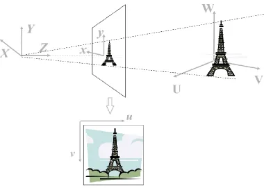
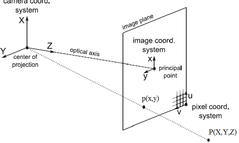
Coordinate Systems

1) World Coordinate (U, V, W)

It is the absolute coordinate system of the world. In general, a 3D scene is expressed

in this coordinate system.

2) Camera Coordinate (X, Y, Z)

This coordinate system is related to the pinhole camera model. In this coordinate

system, Z is the optical axis (or line if sight), with the image plane located at𝑓units

away along the optical axis. 𝑓 is known as the focal length.

3) Film Coordinate (𝑥, 𝑦)

By forward projecting point from camera coordinates onto the image plane, a 2D

coordinate is obtained, which is called a film coordinate.

4) Pixel Coordinate (𝑢, 𝑣)

In images, the points are measured in pixel units, so the film coordinate needs to be

(24)

in the upper left corner of the image and the u and v axes are parallel to x and y axes

in film coordinates.

Figure 3.3 shows the relationship between the four coordinate systems.

Figure 3.3 Projection between different coordinate systems

Pinhole Camera Model

Given a camera coordinate system with 𝑓 as its focal length. The line from center of

projection and perpendicular to the image plane is called principal axis of the camera and

(25)

Assume (𝑋, 𝑌, 𝑍) is the 3D coordinates of an image point p(𝑥, 𝑦) on the camera image

plane. Then, the 3D point and its 2D image point are related as:

𝑥 = 𝑓𝑋

𝑍 , 𝑦 = 𝑓 𝑌

𝑍 (3.2)

This relation is known as perspective projection. However, x and y are expressed in the

units of the world coordinate system, and need to be converted to pixel units.

Transforming the coordinates requires knowing the column-wise and row-wise density of

the pixels (pixels per millimeter), let them be 𝑎_𝑢and 𝑎_𝑣 respectively. We also need to

know the deviation of the principal point from the image center. Let its coordinates be

(−𝑥₀, −𝑦₀). Then p can be written as

𝑢 = 𝑎_𝑢(𝑥 + 𝑥0) = 𝑎𝑢𝑓 𝑋

𝑍+ 𝑎𝑢𝑥0 (3.3)

𝑣 = 𝑎_𝑣(𝑦 + 𝑦₀) = 𝑎_𝑣𝑓𝑌

𝑍+ 𝑎𝑣𝑦0 .

(26)

Figure 3.4 A pinhole camera model.

3.2 Camera Calibration

Intrinsic Parameters

Equation (3.3)

𝑢 = 𝑎_𝑢(𝑥 + 𝑥0) = 𝑎𝑢𝑓 𝑋

𝑍+ 𝑎𝑢𝑥0

𝑣 = 𝑎_𝑣(𝑦 + 𝑦₀) = 𝑎_𝑣𝑓𝑌

𝑍+ 𝑎𝑣𝑦0 .

(27)

𝑃′ =𝑃 𝑍 = ( 𝑋 𝑍 ⁄ 𝑌 𝑍 ⁄ 𝑍 𝑍 ⁄ ) = ( 𝑋′ 𝑌′

1) (3.4)

Then (3.3) can be expressed as:

(𝑢𝑣 1) = (

𝑎𝑢𝑓 0 𝑎𝑢𝑥0

0 𝑎_𝑣𝑓 𝑎_𝑣𝑦₀

0 0 1

) (𝑋

′

𝑌′

1) = 𝐾𝑃

′ _(3.5)

and let

𝑓_𝑥 = 𝑎_𝑢𝑓, 𝑓_𝑦 = 𝑎_𝑣𝑓, 𝑐_𝑥 = 𝑎_𝑢𝑥₀, 𝑐_𝑦 = 𝑎_𝑣𝑦₀.

Those four quantities are determined by the internal structure of the camera, and are

known as intrinsic parameters. Therefore, the camera intrinsic parameter matrix 𝐾 can be

represented as:

𝐾 = (

𝑓_𝑥 0 𝑐_𝑥

0 𝑓_𝑦 𝑐_𝑦

0 0 1

) (3.6)

Normally, the intrinsic parameters of the camera are usually found by calibration [22].

For the Kinect cameras, they can be obtained using the Microsoft Kinect SDK v2.0 [23].

3.2.1.1 Distortion Coefficients

In the section 3.1.3, we introduced the pinhole camera model, disregarding the possibility

of distortions introduced by the camera assembly and the lens itself. Because of such

(28)

There are two types of distortions: optical and perspective. Both result in some type of

image deformations, lightly or noticeably. In optical distortion, there has been two most

common and significant distortions: Barrel Distortion and Pincushion Distortion. Figure

3.5 shows how they deform images.

Figure 3.5 Barrel Distortion and Pincushion Distortion

These distortions are accounted for and corrected with relatively simple models [22],

[24]. Let (𝑥, 𝑦) be the ideal coordinates on image plane, and (𝑥_𝑑, 𝑦_𝑑) the corresponding,

real observed coordinates. Also, let (0,0) denote the principal point, free of any

distortion. Then we can write:

𝑥𝑑 = 𝑥 ∙ (1 + 𝑘1𝑟2+ 𝑘2𝑟4+ 𝑘3𝑟6), (3.7)

𝑦_𝑑 = 𝑦 ∙ (1 + 𝑘₁𝑟2+ 𝑘₂𝑟4+ 𝑘₃𝑟6),

Where

(29)

and𝑘₁, 𝑘₂, 𝑘₃ are radial distortion coeﬃcients. Zhang claims that the first two terms in

these equations are sufficient to adequately undistort images in most cases [2].

3.2.1.2 Extrinsic Parameters

In the pinhole camera model, we have a prerequisite assumption that the center of the

camera coordinate system is the center of world coordinate system. But in real life, it not

always the case. We define a rotation matrix 𝑅 and a translation vector 𝒕⃗ to denote the

coordinate system transformations from 3D world coordinates to 3D camera coordinates.

Let P(𝑈, 𝑉, 𝑊) to be a point in the world coordinate and P(𝑋, 𝑌, 𝑍)corresponding to

coordinates in the camera coordinate system. Then,

( 𝑋 𝑌 𝑍 ) = 𝑅 · ( 𝑈 𝑉 𝑊 ) + 𝒕⃗ = (

𝑟11 𝑟12 𝑟13 𝑟21 𝑟22 𝑟23 𝑟₃₁ 𝑟₃₂ 𝑟₃₃) · (

𝑈 𝑉 𝑊 ) +· ( 𝑡_𝑥 𝑡_𝑦 𝑡𝑧 ) (3.8)

The parameters 𝑅 and 𝒕⃗ are known as extrinsic parameters. They describe the camera's

location and orientation in the world coordinate system. The extrinsic parameters are

often written in a matrix form:

[𝑅|𝒕⃗] = [

𝑟₁₁ 𝑟₁₂ 𝑟₁₃ 𝑟₂₁ 𝑟₂₂ 𝑟₂₃ 𝑟₃₁ 𝑟₃₂ 𝑟₃₃|

𝑡𝑥 𝑡𝑦 𝑡_𝑧

] , (3.9)

(30)

3.3 Epipolar Geometry

3.3.1.1 Overview

When using two cameras or the same camera in two different locations to image the same

scene, the two resulting pictures are related by what is known as Epipolar Geometry. This

type of geometry is independent of scene structure, and only depends on the cameras’

internal parameters and relative pose [25].

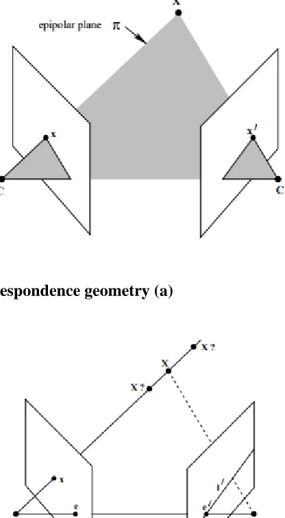
Suppose 𝑋 is a point in 3D world coordinates, where 𝑋 is projected onto the two views,

as 𝑥 in the first view, and as 𝑥′_{in the second view. 3D Point}_𝑋_{and the camera centers}_𝐶

and 𝐶′ form what is known as the epipolar plane 𝜋. Figure 3.6, shows that the rays

back-projected from 𝑥 and 𝑥′ intersect at 𝑋, and are lying in the plane 𝜋.

If we only know 𝑥, the position of 𝑥′_{is impossible to determine (See Figure 3.7). The}

plane 𝜋 is determined by the stereo baseline and the rays defined by 𝑥. The point 𝑥′_lies

on a line 𝑙′, which is the image in the second view of the ray back-projected from x. This

constraint is quite crucial to stereo correspondence, since the search for the point

corresponding to x need not cover the entire image plane but can be restricted to the line

𝑙′_{, known as an epipolar line.}

We introduce the terminology of Epipolar geometry.

➢ Epipole: the epipole is the point of intersection of the line joining the camera centers

(the baseline) with the image plane.

(31)

➢ Epipolar line: an epipolar line is the intersection of an epipolar plane with the image

plane. All epipolar lines intersect at the epipole.

The geometric entities involved in Epipolar geometry are illustrated in Figure 3.8.

Figure 3.6 Points correspondence geometry (a)

(32)

Figure 3.8 Illustration of Epipolar geometry

3.3.1.2 Fundamental and Essential Matrices

In 1981, Longuet-Higgins found that there is a special 3 × 3 matrix that associates two

images from different perspectives of the same scene [26]. Then in the late 1980s and

early 1990s, other scholars re-discovered this matrix in various fields. It came to be

known as the Fundamental Matrix.

Let’s consider two perspective images of a scene as taken from a stereo pair of cameras.

(or equivalently, assume the scene is rigid and imaged with a single camera from two

different locations) and suppose 𝐾𝑙 and 𝐾𝑟 are the intrinsic parameter matrices of these

two cameras. Let P be a point in the world coordinate, and 𝑃_𝑙(𝑃_𝑙_𝑥, 𝑃_𝑙_𝑦, 𝑃_𝑙_𝑧) and

𝑃𝑟(𝑃𝑟𝑥, 𝑃𝑟𝑦, 𝑃𝑟𝑧) be the coordinates of P in left and right camera coordinate system. The

position and orientation of the two cameras are related by a rotation matrix 𝑅 and a

translation vector𝒕⃗ = (𝑡_𝑥, 𝑡_𝑦, 𝑡_𝑧)𝑇in the following way:

(33)

Due to the epipolar constraint (see Figure 3.9) and outer product properties we can write:

𝑃_𝑟∙ (𝒕⃗ × 𝑃_𝑟) = 0 (3.11)

Combining (3.10) and (3.11) yields:

𝑃𝑟∙ (𝒕⃗ × (𝑅 · 𝑃𝑙+ 𝒕⃗)) = 0 (3.12)

Since, 𝒕⃗ × 𝒕⃗ = 𝟎, the equation is equivalent to:

𝑃_𝑟∙ 𝒕⃗ × 𝑅 ∙ 𝑃_𝑙 = 0 (3.13)

We have

𝒕⃗ × 𝑅 = S𝑅 (3.14)

where

𝑆 = [

0 −𝑡_𝑧 𝑡_𝑦 𝑡_𝑧 0 −𝑡_𝑥 −𝑡_𝑦 𝑡_𝑥 0

] ,

is a skew-symmetric matrix of rank 2.

Thus, we write:

𝑃_𝑟𝑇_{∙ 𝑆𝑅 ∙ 𝑃}

𝑙 = 0 . (3.15)

Let 𝐸 = 𝑅𝑆:

(34)

The matrix 𝐸 here called the Essential Matrix. The matrix 𝐸:

 has rank 2, and

 depends only on the extrinsic parameters (𝑹 and 𝒕⃗).

Consider 𝑥_𝑙 = (𝑢_𝑙, 𝑣_𝑙) and 𝑥_𝑟 = (𝑢_𝑟, 𝑣_𝑟) as the projections of 3D point 𝑃 onto the two

image planes, with 𝑥_𝑙 and 𝑥_𝑟 defined as:

𝑥_𝑙 = (𝑢𝑙

𝑣𝑙

1

) , 𝑥_𝑟 = (𝑢𝑟

𝑣𝑟

1

) (3.17)

According to (3.4), we have

𝑍 · 𝑥_𝑙 = 𝐾_𝑙𝑋_𝑙 , (3.18)

𝑍 · 𝑥𝑟 = 𝐾𝑟𝑋𝑟.

Combing (3.16) and (3.18)

𝑍2∙ 𝑥_𝑟𝑇∙ 𝐾_𝑟−𝑇∙ 𝐸 ∙ 𝐾_𝑙−1∙ 𝑥_𝑙 = 0 , (3.19)

which is equivalent to

𝑥_𝑟𝑇_{∙ 𝐾}

𝑟−𝑇∙ 𝐸 ∙ 𝐾𝑙−1∙ 𝑥𝑙= 0 (3.20)

The matrix 𝐹 = 𝐾_𝑟−𝑇_{∙ 𝐸 ∙ 𝐾}

𝑙−1, is called Fundamental Matrix and expresses epipolar

(35)

Figure 3.9 Epipolar constraint

3.4 Feature Detection

SIFT Feature

The Scale Invariant Feature Transform (SIFT) was first proposed by David Lowe in 1999

and improved in 2004 to identify points of interest in an image [2], [3]. The SIFT

approach, for image feature generation, takes an image and transforms it into a "large

collection of local feature vectors", with each of these feature vectors invariant to scaling,

rotation or translation of the image.

The SIFT algorithm consists of a 4-stage filtering approach:

 Scale-space peak detection

This stage of the filtering attempts to identify those locations and scales that are

identifiable from different views of the same object. The approach to achieve this is

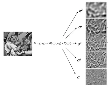
building a scale space by using Laplacian of Gaussian (LoG). The scale space is defined

(36)

𝐿(𝑥, 𝑦, 𝜎_𝐷) = 𝐺(𝑥, 𝑦, 𝜎_𝐷) ∗ 𝐼(𝑥, 𝑦) ,

where 𝐼(𝑥, 𝑦) represents the original image, ∗ is the convolution operator, and 𝐺 is a

Gaussian kernel. Figure (3.10) shows an input image to which a Gaussian kernel is

applied in a successive manner.

There are various techniques to detect stable key point locations in scale-space. One of

them is the Difference of Gaussians technique: locating scale-space peak 𝐷(𝑥, 𝑦, 𝜎𝐷) by

computing the difference between two images, one with scale𝑘 times the other.

𝐷(𝑥, 𝑦, 𝜎_𝐷) is then given by:

𝐷(𝑥, 𝑦, 𝜎_𝐷) = 𝐿(𝑥, 𝑦, 𝑘𝜎𝐷) − 𝐿(𝑥, 𝑦, 𝜎𝐷)

To detect the local maxima and minima of 𝐷(𝑥, 𝑦, 𝜎𝐷), each point is compared with its 8

neighbors at the same scale, and its 9 neighbors up and down one scale. If this value is

(37)

Figure 3.10 Input image applied with different Gaussian kernel. Applied with

different scales factor, input image shows different details.

 Key point localization

The purpose of this step is to pinpoint the location of the feature key. To reach this goal,

the Laplacian value for each key point found in stage 1 is calculated. The location of

extremum, z is given by:

z = −

𝜕

2

_𝐷

−1

𝜕𝑋

2

(38)

If the function value at z is below a threshold value then this point is excluded. By doing

this, low contrast extrema and poorly localized candidates are removed. It is noted for

difference of Gaussian function that there is a large principle curvature across the edge

but a small curvature in the perpendicular direction. If this difference is below the ratio of

largest to smallest eigenvector, from the 2x2 Hessian matrix at the location and scale of

the key point, the key point is rejected.

 Orientation assignment

This is the third step of SIFT. The purpose is to achieve the orientation invariance of the

SIFT feature. The approach taken to find an orientation is:

➢ Use the key points scale to select the Gaussian smoothed image L

➢ Compute gradient magnitude 𝑚 and orientation 𝜃

𝑚(𝑥, 𝑦) = √(𝐿(𝑥 + 1, 𝑦) − 𝐿(𝑥 − 1, 𝑦))2_{+ (𝐿(𝑥, 𝑦 + 1) − 𝐿(𝑥, 𝑦 − 1))}2_,

𝜃(𝑥, 𝑦) = tan−1((𝐿(𝑥, 𝑦 + 1) − 𝐿(𝑥, 𝑦 − 1)) (𝐿(𝑥 + 1, 𝑦) − 𝐿(𝑥 − 1, 𝑦))⁄ )

➢ For each key point, we select the 16 x 16 neighborhood and quantify the gradient of

all pixels (256) in this window into the histogram of 36 bin.

➢ Locate the highest peak in the histogram. Use this peak and any other local peak

within 80% of the height of this peak to create a key point with that orientation

(39)

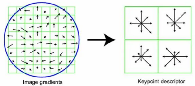
Once Completed the above three steps of SIFT, then we need to find a Local Image

Descriptors at key points. Here we chose to use the gradient direction histogram to

describe this key point. Key point descriptors typically use a set of 16 histograms, aligned

in a 4x4 grid, each with 8 orientation bins, one for each of the main compass directions

and one for each of the mid-points of these directions. This results in a feature vector in

128-dimensions, (see Figure 3.11).

Figure 3.11 SIFT key point descriptor

SURF Feature

In computer vision, speeded up robust features (SURF) is a patented local feature

detector and descriptor. This algorithm is based on the same principles and steps of SIFT,

but it utilizes a different scheme [4].

(40)

SURF uses a Hessian based blob detector [27] to find interest points. The determinant of

a Hessian matrix expresses the extent of the response and is an expression of the local

change around the area.

A Hessian Matrix is defined as:

𝐻(𝑥, 𝜎) = [𝐿𝑥𝑥(𝑥, 𝜎) 𝐿𝑥𝑦(𝑥, 𝜎) 𝐿_𝑥𝑦(𝑥, 𝜎) 𝐿_𝑦𝑦(𝑥, 𝜎)] ,

where

𝐿_𝑥𝑥(𝑥, 𝜎) = 𝐼(𝑥) ∗ 𝜕 2

𝜕𝑥2𝑔(𝜎)

𝐿_𝑥𝑦(𝑥, 𝜎) = 𝐼(𝑥) ∗ 𝜕 2

𝜕𝑥𝑦𝑔(𝜎)

The core of SURF detection is non-maximal-suppression of the determinants of the

Hessian matrices. However, to calculate the convolutions is a time-consuming process.

To speed it up, integral images and approximated kernels are being used.

An Integral image 𝐼(𝑥) is an image where each point 𝑝(𝑥, 𝑦)𝑇stores the sum of all pixels

in a rectangular area between center 𝑂(0,0)𝑇_and_p.

𝐼(𝑥) = ∑ ∑ 𝐼(𝑥, 𝑦) 𝑗<𝑦

𝑗=0 𝑖<𝑥

𝑖=0

(41)

As in the first stage of SIFT, interest points can be found at different scales, partly

because the search for correspondences often requires the comparison of images where

these points are seen at different scales. In the stages of building a scale pyramid, the

SURF and SIFT use different strategies. For SIFT, the Gaussian filter size is kept

unchanged, but the image size changes at different scales. The SURF technique is

opposite, the image size remains unchanged but the filter size changes (see Figure 3.12).

In order to localize interest points in the image and over scales, a non-maximum

suppression in a 3 × 3 × 3 neighborhood is applied.

Figure 3.12 Differences between SIFT (left side) and SURF (right side) when

constructing a scale space.

 Orientation assignment

In order to be invariant to image rotation, SURF builds the distribution of first-order Haar

(42)

The dominant orientation is estimated by calculating the sum of all responses within a

sliding orientation window of size 𝜋⁄₃, as in Figure 3.13.

Figure 3.13 Orientation assignment of SURF. The right region has a strongest Haar

Wavelet response, therefore such orientation serves as the dominant orientation for

the interst point.

 Descriptor based on sum of Haar wavelet responses

For the extraction of the descriptor, the first step consists of constructing a square region

centered around the interest point and oriented along the dominant orientation. The size

of this window is 20s, where s is the scale at which the interest point was detected. The

region is then split up regularly into smaller 4 × 4 square sub-regions. Then, the wavelet

responses 𝑑𝑥, 𝑑𝑦,|𝑑𝑥| and |𝑑𝑦| are summed up over each sub-region and form a feature

(43)

Figure 3.14 Feature descriptor for SURF

3.5 Correspondence

Overview

Given two or more images of the same 3D scene, taken from different points of view, the

correspondence problem refers to the task of finding a set of points in one image which

can be identified as the same points in another image.

There are two basic ways to achieve this:

(44)

The idea of the correlation is to check if one part in one image looks like another in

another image. One simple method is to compare small patches between rectified images:

A filter window is passed over a number of positions in one image to check how well it

compares with the same location as well as several nearby locations in the other image.

 Feature-based methods

This kind of methods first finds features in one image and then associates them with

features from a second image that are most similar. As mentioned in Section 3.4, SIFT,

SURF and other feature point detection algorithms could be used to reach this goal. For

example, rough correspondence could be found by just comparing two key points

descriptor’s Euclidean distance.

Random Sample Consensus (RANSAC)

The RANSAC algorithm performs a robust fitting of models in the presence of many data

outliers [27], [28],[29]. Given a dataset whose data elements contain both inliers and

outliers, RANSAC uses the voting scheme to find the optimal fitting result. The

implementation of this voting scheme is based on two assumptions:

 Few Outliers: the noisy features will not vote consistently for any single model.

 Few Missing Data: there are enough features to agree on a good model.

RANSAC algorithm is often used in computer vision. To be specific, it could be used to

simultaneously solve the correspondence problem and estimate the fundamental

(45)

This algorithm works as follows:

Algorithm:

Input: source RGB-D image 𝐼_𝑙 and 𝐼_𝑟, threshold 𝜀, Maximum iteration 𝜇

Output: high-quality correspondences set 𝑆 and Essential Matrix 𝐸

Step 1: Calculate Feature points set 𝐹_𝑙 and 𝐹_𝑟 from source image. (e.g. using SURF

feature.)

Step 2: Calculate correspondence set𝐶 from 𝐹_𝑙 and 𝐹_𝑟 by using feature based

correspondence methods.

Step 3: Initialize 𝑁 = 0.

Step 4: Randomly select a set 𝑆𝑡 , which contains 8 correspondences, from 𝐶 and

compute 𝐸_𝑡 with 8 points algorithms and initialize 𝑁_𝑡=0.

Step 5: for correspondence 𝑝 ↔ 𝑞 in 𝐶, compute𝑝𝐸_𝑡𝑞.

if 𝑝𝐸_𝑡𝑞 < 𝜀

then 𝑁𝑡 = 𝑁𝑡+ 1

Step 6: if 𝑁_𝑡> 𝑁

then 𝑁 = 𝑁_𝑡, 𝑆 = 𝑆_𝑡, 𝐸 = 𝐸_𝑡.

(46)

Step 8: output set 𝑆 and Essential Matrix 𝐸.

3.6 Camera pose estimation Algorithm

Eight-Points Algorithm (2D-2D)

3.6.1.1 Computing the Fundamental Matrix

In Section 3.1.1.2, we introduced the Fundamental Matrix

𝑥_𝑟𝑇∙ 𝐹 ∙ 𝑥_𝑙 = 0

where 𝑥_𝑟 and 𝑥_𝑙 are projections of the same 3D point in two different image planes.

Given any pair of correspondence 𝑝 ↔ 𝑞 where 𝑝 = (𝑢, 𝑣, 1)𝑇 and 𝑞 = (𝑢′, 𝑣′, 1)𝑇, the

equation relating points p and q to the Fundamental Matrix 𝐹 is:

𝑢𝑢′𝑓11+ 𝑢𝑣′𝑓21+ 𝑢𝑓31+ 𝑣𝑢′𝑓12+ 𝑣𝑣′𝑓22+ 𝑣𝑓32+ 𝑢′𝑓13+ 𝑣′𝑓23+ 𝑓33= 0 .

Each correspondence gives rises to one linear equation in the unknown entries of 𝐹.

Therefore at least 8 correspondences are needed to estimate matrix 𝐹 from a homogenous

set of linear equations:

[

𝑢1𝑢1′ 𝑢1𝑣1′ 𝑢1 𝑣1𝑢1′ 𝑣1𝑣1′ 𝑣1 𝑢1′ 𝑣1′ 1

⋮ ⋮ ⋮ ⋮ ⋮ ⋮ ⋮ ⋮ ⋮

𝑢₈𝑢₈′ 𝑢₈𝑣₈′ 𝑢₈ 𝑣₈𝑢₈′ 𝑣₈𝑣₈′ 𝑣₈ 𝑢₈′ 𝑣₈′ 1

] 𝑓⃗ = 0 . (3.21)

Where 𝑓⃗ = (𝑓₁₁, 𝑓₂₁, 𝑓₃₁, 𝑓₁₂, 𝑓₂₂, 𝑓₃₂, 𝑓₁₃, 𝑓₂₃, 𝑓₃₃)𝑇,

(47)

𝑨𝑓⃗ = 0 (3.22)

we are seeking 𝑓⃗ that minimizes ‖𝑨𝑓⃗‖ subject to the constraint ‖𝑓⃗‖ = 𝑓⃑𝑇∙ 𝑓⃑ = 1. This

represents a least-squares estimation of the Fundamental Matrix.

3.6.1.2 Extracting Camera Pose from the Essential Matrix

Once 𝐹 is estimated, we can compute the Essential Matrix with the following equation:

𝐸 = 𝐾_𝑟𝑇_{∙ 𝐹 ∙ 𝐾} 𝑙

We also have

𝐸 = 𝒕⃗ × 𝑅 = 𝑆𝑅 , (3.23)

where 𝑅 and 𝒕⃗ are the rotation matrix and the translation vector describing the positions

of the two cameras, relative to each other.

𝐸 has the following properties,

 rank 2

 det( 𝐸) = 0

 its two non-zero singular values are equal.

Since the scale is arbitrary, we set a constraint stipulating ‖𝒕⃗‖ = 1.

(48)

𝐸 = 𝑈 ∙ 𝑑𝑖𝑎𝑔(1,1,0) ∙ 𝑉𝑇 _(3.24)

We introduce two auxiliary matrices:

𝑊 = [

0 −1 0

1 0 0

0 0 1

] and 𝑍 = [

0 1 0

−1 0 0

0 0 0

]

where the matrix𝑊 is a rotation and 𝑍 is skew symmetric. Furthermore, for these

matrices we have:

𝑍𝑊 = diag(1,1,0) , (3.25)

𝑍𝑊𝑇 _{= −diag(1,1,0)}

Using (3.23) and (3.24), we have two solutions that fit 𝐸 = 𝑆𝑅, which are

𝑆₁ = −𝑈𝑍𝑈𝑇 , 𝑅₁ = 𝑈𝑊𝑇𝑉𝑇 , (3.26)

𝑆₂ = 𝑈𝑍𝑈𝑇_{, 𝑅}

2 = 𝑈𝑊𝑉𝑇 .

It’s easy to validate that both 𝑅1 and 𝑅2 are rotations and 𝑆1 = 𝑆2. We can extract 𝒕⃗ from

𝑆1(or 𝑆2) such that 𝒕⃗ = ±(𝑠32, 𝑠13, 𝑠21)𝑇.

Therefore, we have four possible solutions of 𝑅 and 𝒕⃗, which are (𝑅₁, 𝒕⃗), (𝑅₂, 𝒕⃗),

(𝑅₁, −𝒕⃗), (𝑅₂, −𝒕⃗), and only one of them is the right solution. Since 𝒕⃗ is normalized to

‖𝒕⃗‖ = 1, the actual translation vector between the two cameras is determined up to a

scale factor: 𝑇 = λ ∙ 𝒕⃗. To solve for the exact camera pose, we need to use 3D point depth

information. Only one of these solutions puts the scene points in front of both cameras.

(49)

triangulation, and choosing the one solution that enforces most of the structure solution

(allowing for a few reconstruction errors) to be in front of both cameras. In Figure 3.15,

only solution 2 has positive depths, thus solution 2 is the correct one.

Figure 3.15 Four solution form decompose Essential Matrix. The correct

solution(right top one) makes the world points P has a positive depth in both camera

(50)

Perspective-n-Point Algorithm (3D-2D)

Perspective-n-Point (PnP) [30] is the problem of estimating the pose of an intrinsically

calibrated camera given a set of n 3D points in the world and their corresponding 2D

projections in the image of the camera. Suppose we have𝒏 3D points in the real scene

and their corresponding 2D image projections. Assuming the intrinsic matrix of the

camera is 𝐾, the perspective projection model for cameras can be described as follows:

𝑠𝑃_𝑐 = 𝐾 [𝑅|𝒕⃗]𝑃_𝑤 (3.27)

where 𝑃_𝑤 = (𝑥, 𝑦, 𝑧, 1)𝑇_{is the homogenous world point;}_𝑃

𝑐 = (𝑢, 𝑣, 1)𝑇 is the

corresponding homogenous image point, s is a scale factor for the image point, R and 𝒕⃗

are the desired rotation matrix and translation vector.

This equation also has an equivalent matrix form:

𝑠 [ 𝑢 𝑣 1

] = [

𝑓_𝑥 0 𝑐_𝑥

0 𝑓_𝑦 𝑐_𝑦

0 0 1

] [

𝑟₁₁ 𝑟₁₂ 𝑟₁₃ 𝑡₁ 𝑟₂₁ 𝑟₂₂ 𝑟₂₃ 𝑡₂ 𝑟31 𝑟32 𝑟33 𝑡3

] [ 𝑥 𝑦 𝑧 1

] . (3.28)

Efficient PnP (EPnP) which was developed by Lepetit [5], is a common method for

solving the general problem of PnP for n ≥ 3.

They introduce the concept of virtual control points, and design the algorithm based on

the notion that each of the n points, also known as reference points, can be expressed as a

(51)

Let those n points whose 3D coordinates are known in the camera coordinate system be

𝑝_ic , 𝑖 = 1, ⋯ , 𝑛 and assume 4 virtual control points expressed as 𝑐𝑗 , 𝑗 = 1, ⋯ ,4.

Then we can express each reference point as a weighted sum of control points:

𝑝_𝑖𝑐 = ∑_𝑗=14 𝑎_𝑖𝑗𝑐_𝑗𝑐, with ∑4_𝑗=1𝑎_𝑖𝑗 = 1 (3.29)

Combining with (3.28), we obtain:

∀𝑖 , 𝑠_𝑖[ 𝑢_𝑖 𝑣_𝑖 1

] = [

𝑓𝑥 0 𝑐𝑥

0 𝑓𝑦 𝑐𝑦

0 0 1

] ∑4_𝑗=1𝑎_𝑖𝑗[ 𝑥_𝑗𝑐 𝑦_𝑗𝑐 𝑧_𝑗𝑐

] (3.30)

Substituting this expression in the ﬁrst two rows yields two linear equations for each

reference point:

∑4_𝑗=1𝑎_𝑖𝑗𝑓_𝑥𝑥_𝑗𝑐 + 𝑎_𝑖𝑗(𝑐_𝑥− 𝑢_𝑖)𝑧_𝑗𝑐 _{= 0} _(3.31)

∑4_𝑗=1𝑎_𝑖𝑗𝑓_𝑥𝑦_𝑗𝑐 + 𝑎_𝑖𝑗(𝑐_𝑦− 𝑣_𝑖)𝑧_𝑗𝑐 = 0

Note that projective parameter 𝑠𝑖 disappear in those equations. Grouping all references

points, we generate a linear system:

M𝑥 = 0 (3.32)

Where 𝑥 = [𝑐₁𝑐𝑇, 𝑐₂𝑐𝑇, 𝑐₃𝑐𝑇𝑐₄𝑐𝑇]𝑇 is a vector in 𝑅12 (the coordinates of those control points

are unknown), and M is a 2n × 12 matrix generated by arranging the coefﬁcients of (3.31)

for each reference point.

The solution is to the null space of M, which can be expressed as:

𝑥 = ∑𝑁_𝑖=1𝛽_𝑖𝑣_𝑖 (3.33)

The solution is found efﬁciently by solving the null eigenvectors of matrix 𝑀𝑇_𝑀_.

(52)

In order to have an optimized result, those four coefficients β = [𝛽₁, 𝛽₂, 𝛽₃, 𝛽₄] are

refined by choosing the values that minimize the change in distance between control

points, using Gauss-Newton Optimization:

Error( β) = ∑_{(𝑖,𝑗) 𝑠.𝑡. 𝑖<𝑗}(‖𝑐_𝑖𝑐− 𝑐_𝑗𝑐‖2− ‖𝑐_𝑖𝑤 − 𝑐_𝑗𝑤‖2) (3.34)

where 𝑐_𝑖𝑤 are 3D world coordinates.

After determining the best 𝛽, 𝑥 is solved. Therefore, the pose transformation between the

world coordinates system and the camera coordinate system is easily formed.

This algorithm is found in the open source library OpenCV (routine name: solvePnP).

Also, RANSAC can be used to deal with outliers in the data set to optimize the result

(routine name, solvePnPRansc) [31].

Point Set Registration (3D-3D)

3D Registration is a method to seek for the optimal rotation and translation between two

sets of corresponding 3D point data, that makes them well registered [32]. Suppose we

have two sets of 3D points, dataset A and B. This method has three main steps:

 Finding the centroids

This is quite straightforward: the centroids are the average point and can be calculated as

follows: 𝑐𝑒𝑛𝑡𝑟𝑜𝑖𝑑𝐴 = 1 𝑁∑ 𝑃𝐴 𝑖_, 𝑁 𝑖=1 (3.35)

𝑐𝑒𝑛𝑡𝑟𝑜𝑖𝑑_𝐵 = 1

(53)

Here, 𝑃_𝐴 and 𝑃_𝐵 are points in dataset A and B respectively.

 Finding the optimal rotation

To find the optimal rotation, we need to re-center the datasets so that their centroids are at

the origin. This is shown in Figure 3.16.

Figure 3.16 Re-center dataset

The next step involves the computation of a covariance matrix 𝐻, and using SVD to find

the rotation as follows:

𝐻 = ∑𝑁𝑖=1(𝑃_𝐴𝑖 − 𝑐𝑒𝑛𝑡𝑟𝑜𝑖𝑑𝐴)(𝑃𝐵𝑖 − 𝑐𝑒𝑛𝑡𝑟𝑜𝑖𝑑𝐵)𝑇 (3.36)

[𝑈, 𝑆, 𝑉𝑇_{] = 𝑆𝑉𝐷(𝐻)} _(3.37)

The optimal rotation can be calculated as

𝑅 = 𝑉𝑇_𝑈𝑇 _(3.38)

(54)

R here has to be a rotation matrix, which means ‖𝑅‖ = 1. We need to validate this

property in case the SVD returns a reflection matrix, which is numerically correct but is

nonsense for real cases. If R is the reflection matrix, then ‖𝑅‖ = −1, and we multiply the

third column of R by -1 as a remedy.

 Finding the translation vector

Since we have the optimal R, the translation vector 𝒕⃗ is obtained with:

(55)

Chapter 4

4

Methodology

This thesis proposes to evaluate the algorithms described in the last Section to calibrate

for the extrinsic parameters of two Kinect cameras. In this Section, we follow with

appropriate justifications for our approach, and what the advantages are for each chosen

method or process. Also, this Section justifies the reasons for our choices in the

experiments that follow in the next Chapter.

4.1 Feature Selection

In section 3.4, we presented the SIFT and SURF algorithms. They are quite similar in the

generating phase. In our case, SIFT has detected larger numbers of features compared to

SURF but with slower speed. For its high speed and relatively high-quality performance,

we choose SURF as our feature point detection approach [33].

4.2 Correspondence Method Selection

In the selection of correspondence methods, feature-based methods provide relatively

accurate information about local regions of interest and thus achieve better matching

compared to correlation-based methods, which are also computationally expensive.

Feature-based methods work best with images taken with roughly the same point of view

and either at the same time or with little to no movement of the scene between image

(56)

4.3 Experiments with Real RGB-D Images

Normally, camera pose estimation techniques are aimed at calibrating multiple cameras

in different positions. However, one equivalent way to validate a calibration algorithm is

to keep the scene unchanged and capture images from different positions with one

camera. By doing so, we only need to calibrate intrinsic parameters once, with no

synchronization issues. The experiments in this thesis are based on the second method.

Case 1

For this case, we manually set the pose of the Kinect camera and measure the distance of

the two successive locations used to take images. Since the rotation is hard to physically

measure, we did not rotate the camera. The objective for this case is to prove that the

camera pose obtained by the algorithm is close to the physically measured distance.

Case 2

In this case, we investigate how our algorithm performs in random cases. So, the camera

position is chosen with no particular preference, and the square error of the computed 3D

correspondence sets is calculated to estimate the correctness of the results. Note that the

choice of camera positions is constrained by the fact that there must be a scene overlap in

(57)

4.4 Robustness Analysis

We are interested in finding out the behavior of the algorithms when confronted to noise.

In order to compare the robustness of camera pose estimation algorithms, we used a

synthetic set of 3D points, with a known rotation and translation to also generate the

second 3D set. Noise is then added, and we compare the so obtained translation and

rotation to the original one. We proceed to list the specifics of our robustness analysis.

 Gaussian Noise

Gaussian noise is a random form of noise with a probability density function equal to that

of the normal distribution. In the field of Computer Vision, Gaussian noise is widely used

since it is regarded as the most realistic simulation of noise for most circumstances.

 Synthetic Data

The goal of the robustness experiments is to analyze how algorithms behave when noise

is present. To achieve this goal, we tested the algorithms without the use of the cameras,

to avoid any unwanted noise such as that introduced when finding image

correspondences. The use of synthetic 3D points sets and camera position and orientation

reflects robustness in an unbiased fashion and allows us to know the real total amount of

noise that is being introduced.

 Offsets of R and 𝒕⃗

The rotation matrix is completely specified by three angles about the x-, y-, and z- axes,

which we denote as 𝜃𝑥, 𝜃𝑦 and 𝜃𝑧. We use 𝜃0 = (𝜃𝑥0, 𝜃𝑦0, 𝜃𝑧0)

𝑇_and_𝑡

0 = (𝑡𝑥0, 𝑡𝑦0, 𝑡𝑧0)

(58)

as the ground truth for the rotation angle vector and the translation vector, and 𝜃 =

(𝜃_𝑥, 𝜃_𝑦, 𝜃_𝑧)𝑇_and_{𝑡 = (𝑡}

𝑥, 𝑡𝑦, 𝑡𝑧)𝑇as the results obtained from the algorithms under study.

To measure the system behavior towards noise, the offsets of R and 𝒕⃗ is defined as follow:

Offset_R = √(𝜃 − 𝜃0)𝑇∙ (𝜃 − 𝜃0)

Offset_T = √(𝑡 − 𝑡0)𝑇∙ (𝑡 − 𝑡0)

(59)

Chapter 5

5

Experiments and Results

To properly identify the correctness and the robustness of the algorithms, a series of

experiments are performed in the indoor lab scene. The input for the first experiment are

RGB-D images obtained from our Kinect sensor. This experiment aims to prove that our

work is not only numerically correct but also well suited for general cases. The second

experiment focuses on the robustness of the chosen camera pose estimation algorithms.

Various levels of Gaussian noise are added to the synthetic data and the distance between

the synthetic pose parameters and the output of each algorithm is calculated.

Figure 5.1 shows the type of RGB-D images used for the experiments. The left image is

the RGB image from the color camera, which is resized to 512 × 424 (original resolution

1920 × 1080). The right image is the depth image-capture from the IR sensor, which

also has a resolution of 512 × 424. The red points inside the image indicate invalid depth

values. The intensity of the depth value is related to object distance: nearer surfaces are

(60)

Figure 5.1 RGB-D image structure. The red dots indicate invalid depth value. RGB

image and Depth image has slightly difference if you look carefully (only

demonstrate the RGB-D image structure), they do have intrinsic mapping function

from each RGB pixel to depth pixel.

5.1 Results with Real RGB-D Data

Case 1

In this case, the Kinect sensor first captured an indoor scene at one location and was then

relocated along the 𝑥 axis of the camera coordinate system by approximately 3 inches

(76.2 mm). These two RGB-D images only contain a slight perspective difference, which

makes feature points easy to match correctly. The SURF features (colored dots) from the

image obtained at the second camera position are shown in Figure 5.2 and the optimized

correspondences between the two RGB-D image sources are displayed in Figure 5.3.

Table 2 gives the rotation matrix and translation vector obtained from each specific

(61)

that, in this case, all the algorithms give a nearly perfect solution for the rotation matrix,

which is very close to identity matrix. However, for the translation vector, the

Perspective-n-points algorithm and the 3D point registration algorithm both perform

better than the Eight-point algorithm. These results support the correctness of the

implementations. Moreover, it also indicates that the intrinsic parameters of the camera

are well measured so that the points in the image plane could be adequately re-projected

(62)

Figure 5.2 Case 1: Feature Points. The bottom images zoom in the black region of

the top one. Those colorful dots are SURF feature points detected from feature

(63)

Figure 5.3 Case 1: Correspondences. The bottom images zoom in the black region of

the top one, which shows the details of matching correspondence.

Table 2 Comparison of results from different camera pose estimation algorithms

Algorithms Rotation Matrix Translation Vector

Eight-Point

Algorithm

[

0.9992 −0.0050 0.0398

0.0053 0.9999 0.0074

−0.0398 0.0076 0.9992

] [ −0.0908 0.0215 −0.0083 ] Perspective-n-Point Algorithm [

1.0000 0.0004 −0.0008

−0.0004 0.9999 0.0059

0.0008 −0.0059 1.0000

] [

−0.0804 0.0022 −0.0018

(64)

3D Point

Registration

[

0.9999 −0.0005 −0.0028

0.0005 0.9999 0.0076

0.0028 −0.0076 0.9999

] [ −0.0734 −0.0015 −0.0030 ] Pre-given Ground Truth [

1.0000 0.0000 0.0000

0.0000 1.0000 0.0000

0.0000 0.0000 1.0000

] [ −0.7620 0.0000 0.0000 ]

Case 2

In this case, the Kinect senor is placed at two random locations where the two

perspectives have a visual overlap over the scene. Figures 5.4 and 5.5 show the feature

points and their correspondences separately.

Comparative results from the camera pose estimation algorithms are displayed in Table 3.

Since we no longer have synthetic pose data (rotation and translation), the average

squared error is recorded to measure the performance of each algorithm. The average

squared error is calculated in the following way: For all the matching pairs in the

correspondence set, we use the rotation matrix and the translation vector produced by

each algorithm to re-project the 3D matching points in the left image into a new 3D point

set and then we average the squared error of the re-projection and with the right image

matching points.

From Table 3 we conclude that the Perspective-n-points algorithm and the 3D point

(65)

The result from the Eight-Point algorithm is significantly higher, which is around 0.0775.

However, this error rate is still acceptable.

Figure 5.4 Case 2: Feature Points

(66)

Table 3 Comparative results from different camera pose estimation algorithms

Algorithms Rotation Matrix Transit

Vector Average Squared Error Eight-Points Algorithm [

0.9983 −0.0237 0.0520

0.0097 0.9967 0.2538

−0.0563 −0.2528 0.9659

] [ −0.1508 −0.6120 −0.0477 ] 0.07746700 Perspective-n-Point Algorithm [

0.9985 −0.0186 0.0506

0.0053 0.9679 0.2512

−0.0537 −0.2506 0.9666

] [ −0.2034 −0.5638 −0.0517 ] 0.00492257 3D Points Registration [

0.9986 −0.0187 0.0501

0.0056 0.9674 0.2531

−0.0533 −0.2525 0.9661

] [ −0.2033 −0.5719 −0.0488 ] 0.00473059

5.2 Robustness Analysis

In this experiment, we randomly generate a Kinect-like set of (𝑢, 𝑣, 𝑑) points with 𝑢 ∈

(0,1920), 𝑣 ∈ (0,1080), 𝑑 ∈ (500,8000) (see Table 4). These points, along with the

intrinsic parameters form a set of points 𝑆₁in the world coordinate system.

In addition, we also defined a rotation matrix 𝑅 and a translation vector 𝒕⃗ as ground truth,

where

𝑅 = [

0.684718 0.136252 0.715959

0.492042 0.638267 −0.592039

−0.537639 0.757661 0.369991

(67)

𝒕⃗ = [ 0.35 −0.28

0.76 ]

For all the points in the set 𝑆₁, we follow the convention that𝑞 = 𝑅 ∙ 𝑝 + 𝒕⃗, forming set

𝑆₂which is the perfect matching set for 𝑆₁.

The next step is to add the Gaussian noise in. We defined our levels of Gaussian noise

with various standard deviations, but kept the mean to 0. Figure 5.6 shows how the

Gaussian distribution behaves with different standard deviations.

We form the correspondence sets 𝐺₁ and 𝐺₂ by generating Gaussian noise and adding it

to the points in 𝑆1 and 𝑆2. The noise could be interpreted as the error in dealing with real

case usage, which may come from data gathering, parameter measuring, feature matching

and so on.

We then input 𝐺1 and 𝐺2 into the camera pose estimation stage of our chosen algorithms

and record the offsets between the outputs and the pre-set ground truth values. Note that,

when sigma equals to 0, both algorithms give nearly error-free solutions, as expected.

The results are shown in Figures 5.7 and 5.8. From these, we conclude that each

algorithm has a different tolerance to input noise. The 3D Registration algorithm

performs best when faced with noise, as the offset for both R and T is close to 0 if sigma

is less than 0.6. The Perspective-n-points algorithm’s output is a relatively precise result

if the noise level (sigma) is less than 0.4. The Eight-point algorithm is very sensitive to

noise. Even a tiny amount of noise has a great influence on the results. Only when sigma

Feature Based Calibration of a Network of Kinect Sensors

Scholarship@Western

Scholarship@Western

Feature Based Calibration of a Network of Kinect Sensors

Feature Based Calibration of a Network of Kinect Sensors

Keywords

Acknowledgments

Table of Contents

List of Tables

List of Figures

Chapter 1

1

Introduction

1.1

Overview

1.2

Kinect Mechanism

Kinect Sensing Hardware

1.3

Problem and Issues

1.4

Thesis Contribution

1.5

Thesis Contents

Chapter 2

2

Related Work

Chapter 3

3

System Description

3.1

Stereo Vision Theory

Disparity and Depth

z =

=

Coordinate Systems

Pinhole Camera Model

3.2

Camera Calibration

Intrinsic Parameters

3.2.1.1

Distortion Coefficients

3.2.1.2

Extrinsic Parameters

3.3

Epipolar Geometry

3.3.1.1

Overview

3.3.1.2

Fundamental and Essential Matrices

3.4

Feature Detection

SIFT Feature

z = −

𝜕

𝐷

𝜕𝑋

SURF Feature

3.5

Correspondence

Overview

Random Sample Consensus (RANSAC)

3.6

Camera pose estimation Algorithm

Eight-Points Algorithm (2D-2D)

3.6.1.1

Computing the Fundamental Matrix

3.6.1.2

Extracting Camera Pose from the Essential Matrix

Perspective-n-Point Algorithm (3D-2D)

Point Set Registration (3D-3D)

Chapter 4

4

Methodology

4.1

Feature Selection

4.2

Correspondence Method Selection

4.3

Experiments with Real RGB-D Images

_𝐷