Robust learning in random subspaces: equipping NLP for
OOV effects
Anders Søgaard and Anders Johannsen
Center for Language Technology
University of Copenhagen
DK-2300 Copenhagen S
{
soegaard
|
ajohannsen
}
@hum.ku.dk
A
BSTRACTInspired by work on robust optimization we introduce a subspace method for learning linear classifiers for natural language processing that are robust to out-of-vocabulary effects. The method is applicable in live-stream settings where new instances may be sampled from dif-ferent and possibly also previously unseen domains. In text classification and part-of-speech (POS) tagging, robust perceptrons and robust stochastic gradient descent (SGD) with hinge loss achieve average error reductions of up to 18% when evaluated on out-of-domain data.
1 Introduction
In natural language processing (NLP), data is rarely drawn independently and identically at random. In particular we often apply models learned from available labeled data to data that differs from the original labeled data in several respects. Supervised learning without the assumption that data is drawn identically is sometimes referred to astransfer learning, i.e. learning to make predictions about data sampled from a target distribution using labeled data from arelated, but different source distributionor under a strongsample bias.
Domain adaptationrefers to a prominent class of transfer learning problems in NLP. Two
domain adaptation scenarios are typically considered: (a)semi-superviseddomain adaption, where a small sample of data from the target domain is available, as well as large pool of unlabeled target data, and (b)unsuperviseddomain adaptation where only unlabeled data is available from the target domain. In this paper we donot evenassume the latter, but consider the more difficult scenario where the target domain is unknown.
The assumption that a large pool of unlabeled data is available from a relatively homogeneous target domain holds only if the target domain is known in advance. In a lot of applications of NLP, this is not the case. When we design publicly available software such as the Stanford Parser, or when we set up online services such as Google Translate, we do not know much about the input in advance. A user will apply the Stanford Parser to any kind of text from any textual domain and expect it to do well.1 Recent work has extended domain adaptation with domainidentification(Dredze et al., 2010; McClosky et al., 2010), but this still requires that we know the possible domains in advance and are able to relate each instance to one of them, and in many cases we do not. If the possible target domains arenotknown in advance, the transfer learning problem reduces to the problem of learning robust models that are as insensitive as possible to domain shifts. This is the problem considered in this paper. One of the main reasons for performance drops when evaluating supervised NLP models on out-of-domain data is out-of-vocabulary (OOV) effects (Blitzer et al., 2007; Daumé and Jagarlamudi, 2011). Several techniques for reducing OOV effects have been introduced in the literature, including spelling expansion, morphological expansion, dictio-nary term expansion, proper name transliteration, correlation analysis, and word clustering (Blitzer et al., 2007; Habash, 2008; Turian et al., 2010; Daumé and Jagarlamudi, 2011), but most of these techniques still leave us with a lot of "empty dimensions", i.e. features that are always 0 in the test data. While these features are not uninstantiated in the sense of missing values, we will nevertheless refer to OOV effects asremoving dimensionsfrom our datasets, since a subset of dimensions become uninformative as we leave our source domain.
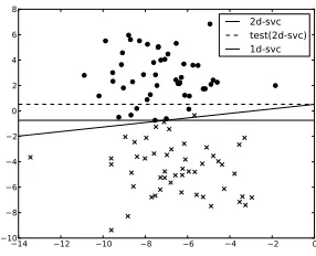
This is a potential source of error, since the best decision boundary inndimensions is not necessarily the best boundary inm<ndimensions. If we remove dimensions, our optimal decision boundaries may suddenly be far from optimal. Consider, for example, the plot in Figure 1. 2D-SVC is the optimal decision boundary for this two-dimensional dataset (the non-horizontal, solid line). If we remove one dimension, however, say because this variable is never instantiated in our test data, the learned weight vector will give us the decision bound-aryTEST(2D-SVC) (the dashed line). Compare this to the optimal decision boundary for the reduced, one-dimensional dataset, 1D-SVC (the horizontal, solid line).
−14 −12 −10 −8 −6 −4 −2 0 −10
−8 −6 −4 −2 0 2 4 6 8
2d-svc test(2d-svc) 1d-svc
Figure 1: Optimal decision boundary is not optimal when one dimension is removed
mensions are to be removed in our target data in advance, however. In this paper we therefore, inspired by previous work on robust optimization (Ben-Tal and Nemirovski, 1998), suggest to minimize our expected loss under all (orKrandom) possible removals. We will implement this strategy for perceptron learning and SGD with hinge loss and apply it to text classification, as well as POS tagging. Results are very promising, with error reductions up to 70% and average error reductions up to 18%.
2 Robust learning under random subspaces
In robust optimization (Ben-Tal and Nemirovski, 1998) we aim to find a solutionwthat min-imizes a (parameterized) cost function f(w,ξ), where the true parameterξmay differ from the observedξˆ. The task is to solve
min w maxξˆ∈∆
f(w,ξˆ) (1)
with∆all possible realizations ofξ. An alternative to minimizing loss in the worst case is minimizing loss in the average case, or the sum of losses:
min w
X
ˆ ξ∈∆
f(w,ξˆ) (2)
The learning algorithms considered in this paper aim to learn modelswfrom finite samples (of sizeN) that minimize the expected loss on a distributionρ(with, say,Mdimensions):
min
1: X={〈yi,xi〉}Ni=1
2: fork∈Kdo
3: w0=0,v=0,i=0
4: ξ←random.bits(M)
5: forn∈Ndo
6: ifsign(w·x◦ξ)6=ynthen
7: wi+1←update(wi)
8: i←i+1
9: end if
10: end for
11: v←v+wi
12: end for
13: return w=v/(N×K)
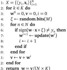
Figure 2: Robust learning in random subspaces
likely to be suboptimal, as discussed in the introduction. In this paper we will instead minimize average expected lossunder random subspaces:
min w
X
ˆ ξ∈∆
E〈y,x〉∼ρL(y, sign(w·x◦ξˆ)) (4)
We refer to this idea as robust learning in random subspaces (RLRS). Since the number of possible instantiations ofξis 2Mwe randomly sampleKinstantiations removing 10% of the dimensions, withK≤250.2
RLRS can be applied to any linear model, and we present the general form in Figure 2. Given a datasetX={〈yi,xi〉}Ni=1we randomly drawξfrom the set of binary vectors of lengthM. We now pass over{〈yi,xi◦ξ〉}Ni=1Ktimes, updating our linear model according to the learning algorithm. The weights of theKmodels are averaged to minimize the average expected loss in random subspaces. In our experiments we will use perceptron (Rosenblatt, 1958) and SGD with hinge loss (Zhang, 2004) as our learning algorithms. A perceptroncconsists of a weight vectorwwith a weight for each feature, a bias termband a learning rateα. For a data point
xj,c(xj) =1 iffw·x+b>0, else 0. The threshold for classifying something as positive is thus−b. The bias term is left out by adding an extra variable to our data with fixed value -1. The perceptron learning algorithm now works by maintainingwin several passes over the data (see Figure 2). Say the algorithm at timeiis presented with a labeled data point〈xj,yj〉. The current weight vectorwiis used to calculatex
j·wi. If the prediction is wrong, an update occurs:
wi+1←wi+α(y
j−sign(wi·xj))xj (5) The numbers of passesKthe learning algorithm does (if it does not arrive at a perfect separa-tor any earlier) is typically fixed by a hyper-parameter. The number of passes is fixed to 5 in our experiments below. The RLRS variant of the perceptron (P-RLRS) is obtained by replacing 2Our choice to constrain ourselves to instantiations ofξremoving 10% of the dimensions was somewhat arbitrary,
−4 −3 −2 −1 0 1 2 3 4 −3
−2 −1 0 1 2 3
perc r-perc
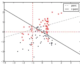
Figure 3: Robust learning in random subspaces (Perceptron on artificial data)
line 8 in Figure 2 with Equation 5. The application of P-RLRS to an artificial two-dimensional dataset in Figure 3 (the solid line) illustrates how P-RLRS can lead to very different decision boundaries than the regular perceptron (the black dashed line) by averaging decision bound-aries learned in random subspaces (red dashed lines).
A perceptron finds the vectorwthat minimizes the expected loss on training data where the loss function is given by:
L(y, sign(w·x)) =max{0,−y(w·x)} (6)
which is 0 wheny is predicted correctly, and otherwise the confidence in the mis-prediction. This reflects the fact that perceptron learning is conservative and does not update on correctly classified data points. Equation 6 is the hinge loss withγ=0. SGD uses hinge loss withγ=1 (like SVMs) (Zhang, 2004). Our objective function thus becomes:
min w
X
ˆ ε∈∆
E〈y,x〉∼ρmax{0,γ−y(w·x◦ξˆ)) (7)
withγ=0 for the perceptron andγ=1 for SGD. We call the RLRS variant of SGD SGD-RLRS.
3 Evaluation
In our experiments we use perceptron and SGD with hinge loss, regularized using theL2-norm. Since we want to demonstrate the general applicability of RLRS, we use the default parameters in a publicly available implementation of both algorithms.3Both algorithms do five passes over the data. SGD uses ’optimal’ learning rate, and perceptron uses a learning rate of 1.
Text classification. The goal of text classification is the automatic assignment of documents into predefined semantic classes. The input is a set of labeled documents〈y1,x1〉, . . . ,〈yN,xN〉, and the task is to learn a functionf :X 7→ Y that is able to correctly classify previously unseen documents. It has previously been noted that robustness is important for the success of text
⊤
comp rec sci talk other
sys others sport vehicles politics religion
(a) (b) (c) (d) (e) (f) (g) (h)
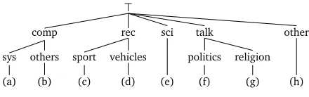
Figure 4: Hierarchical structure of 20 Newsgroups. (a) IBM, MAC, (b) GRAPHICS, MS-WINDOWS, X-WINDOWS, (c) BASEBALL, HOCKEY, (d) AUTOS, MOTORCYCLES, (e) CRYPTOGRAPHY, ELECTRONICS, MEDICINE, SPACE, (f) GUNS, MIDEAST, MISCELLANEOUS, (g) ATHEISM, CHRISTIANITY, MISCELLA -NEOUS, (h) FORSALE
classification in down-stream applications (Lipka and Stein, 2011). In this paper we use the 20 Newsgroups dataset.4 The topics in 20 Newsgroups are hierarchically structured, which enables us to do domain adaptation experiments (Chen et al., 2009; Sun et al., 2011) (except that we will not assume unlabeled data is available in the target domain). See the hierarchy in Figure 4. We extract 20 high-level binary classification problems by considering all pairs of top-level categories, e.g. COMPUTERS-RECREATIVE(comp-rec). For each of these 20 problems, we have different possible datasets, e.g. IBM-BASEBALL, MAC-MOTORCYCLES, etc. Aproblem
instancetakes training and test data from twodifferentdatasets belong to the same high-level problem, e.g. MAC-MOTORCYCLESand IBM-BASEBALL. In total we have 280 available problem instances in the 20 Newsgroups dataset. For each problem instance, we create a sparse matrix of occurrence counts of lowercased tokens and normalize the counts using TF-IDF in the usual way. Otherwise we did not do any preprocessing or feature selection. The code necessary to replicate our text classification experiments is available from the main author’s website.5
POS tagging. To supplement our experiments on the 20 Newsgroups corpus, we also evaluate our approach to robust learning in the context of discriminative HMM training for POS tagging using averaged perceptron (Collins, 2002). The goal of POS tagging is to assign sequences of labels to words reflecting their syntactic categories. We use a publicly available and easy-to-modify reimplementation of the model proposed by Collins (2002).6 We evaluate our tagger on the English Web Treebank (EWT; LDC2012T13). We use the original PTB tag set, and our results are therefore not comparable to those reported in the SANCL 2012 Shared Task of Parsing the Web. Our model is trained on the WSJ portion of the Ontonotes 4.0 (Sect. 2-21). Our initial experiments used the Email development data, but we simply applied document classification parameters with no tuning. We evaluate our model on test data in the remaining sections of EWT: Answers, Newsgroups, Reviews and Weblogs.
3.1 Results and discussion
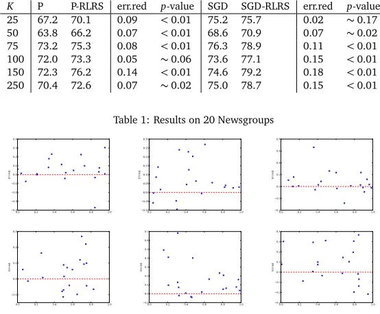
Figure 1 presents our main results on text classification. The left column is the number of extracted subspaces (Kin Figure 2). Note that rows are not comparable, since the 20/280 problem instances were randomly selected for each experiment. Neither are the perceptron and SGD results. We observe that P-RLRS consistently outperforms the regular perceptron
4http:
//people.csail.mit.edu/jrennie/20Newsgroups/ 5http://cst.dk/anders
K P P-RLRS err.red p-value SGD SGD-RLRS err.red p-value
Table 1: Results on 20 Newsgroups
0.0 0.2 0.4 0.6 0.8 1.0
Figure 5: Plots of P-RLRS error reductions withK=25 (upper left),K=50 (upper right), K=75 (lower left),K=100 (lower mid),K=150 (lower mid) andK=250 (lower right).
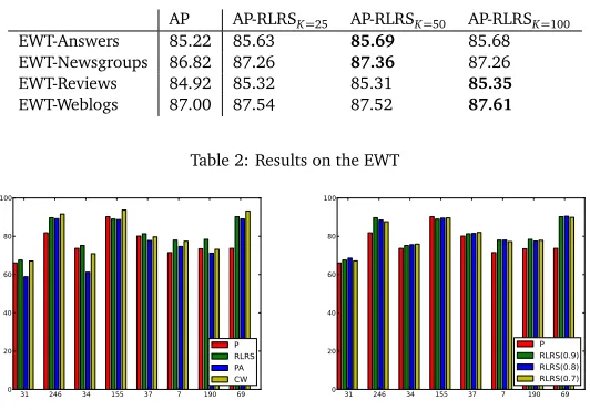
(P), with error reductions of 7–14%. SGD-RSRL consistently outperforms SGD, with error reductions of 2–18%. Note that statistical significance isacross datasets, not across data points. Since we are interested in the probability of success on new datasets, we believe this is the right way to evaluate our model, putting our results to a much stronger test. All results, except two, are still statistically significant, however. As one would expect our models become more robust the more instantiations ofξwe sample. The error reductions for each problem instance in the P/P-RLRS experiments are plotted in Figure 5. The plots show that error reductions are up to 70% on some problem instances, and that RLRS seldom hurts (in 3-8 out of 20 cases). We include a comparison with state-of-the-art learning algorithms for completeness. In Fig-ure 6 (left), we compare SGD-RLRS to passive-aggressive learning (PA) (Crammer et al., 2006) and confidence-weighted learning (CW) (Dredze et al., 2008), using a publicly available im-plementation,7on randomly chosen 20 Newsgroups problem instances. CW is known to be relatively robust to sample bias, reducing weights under-training for correlating features. All algorithms did five passes over the data. Our results indicate that RLRS is more robust than other algorithms, but on some datasets algorithms CW performs much better that RLRS. The results on the EWT are similar to those for 20 Newsgroups, and we observe consistent improvements with both robust averaged perceptron. The results are presented in Table 2. All
AP AP-RLRSK=25 AP-RLRSK=50 AP-RLRSK=100 EWT-Answers 85.22 85.63 85.69 85.68 EWT-Newsgroups 86.82 87.26 87.36 87.26 EWT-Reviews 84.92 85.32 85.31 85.35
EWT-Weblogs 87.00 87.54 87.52 87.61
Table 2: Results on the EWT
31 246 34 155 37 7 190 69
Figure 6: Left: Classifier comparison. Right: Using increased removal rates when samplingξ.
improvements are statistically significant across data points.
As mentioned, fixing the removal rate to 10% when randomly samplingξ∈∆was a relatively arbitrary choice. RLRS actually benefits slightly from increasing the removal rate. See Figure 6 (right) for results on the selection of problem instances we used in our classifier comparison. In order to explain this we investigated and found a statistically significant correlation between the empirical removal rate and the difference in performance of a model with removal rate 0.8 over a model with removal rate 0.9. This, in our view, suggests that the intuition behind RLRS is correct. Learning under random subspacesisa way of equipping NLP for OOV effects.
Related work. The RLRS algorithm in Figure 2 is essentially an ensemble learning algorithm, similar in spirit to the random subspace method (Ho, 1998), except averaging over multi-ple models rather than taking majority votes. Ensemble learning is known to lead to more robust models and therefore to performance gains in domain adaptation (Gao et al., 2008; Duan et al., 2009), so in a way our results are maybe not that surprising. There is also a connection between RLRS and feature bagging (Sutton et al., 2006), a method proposed to reduce weights under-training as an effect of indicative features swamping less indicative fea-tures. Weights under-training makes models vulnerable to OOV effects, and feature bagging, in which several models are trained on subsets of features and combined using a mixture of experts, is very similar to RLRS. Sutton et al. 2006 use manually defined rather than random subspaces. See Smith et al. 2005 for an interesting predecessor.
4 Conclusion
References
Ben-Tal, A. and Nemirovski, A. (1998). Robust convex optimization. Mathematics of Opera-tions Research, 23(4).
Blitzer, J., Dredze, M., and Pereira, F. (2007). Biographies, bollywood, boom-boxes and blenders: Domain adaptation for sentiment classification. InACL.
Chen, B., Lam, W., Tsang, I., and Wong, T.-L. (2009). Extracting discriminative concepts for domain adaptation in text mining. InKDD.
Collins, M. (2002). Discriminative training methods for hidden markov models. InEMNLP.
Crammer, K., Dekel, O., Keshet, J., Shalev-Shwartz, S., and Singer, Y. (2006). Online passive-agressive algorithms.Journal of Machine Learning Research, 7:551–585.
Daumé, H. and Jagarlamudi, J. (2011). Domain adaptation for machine translation by mining unseen words. InACL.
Dredze, M., Crammer, K., and Pereira, F. (2008). Confidence-weighted linear classification. InICML.
Dredze, M., Oates, T., and Piatko, C. (2010). We’re not in Kansas anymore: detecting domain changes in streams. InEMNLP.
Duan, L., Tsang, I., Xu, D., and Chua, T.-S. (2009). Domain adaptation from multiple sources via auxilliary classifiers. InICML.
Gao, J., Fan, W., Jiang, J., and Han, J. (2008). Knowledge transfer via multiple model local structure mapping. InKDD.
Habash, N. (2008). Four techniques for online handling of out-of-vocabulary words in Arabic-English statistical machine translation. InACL.
Ho, T. K. (1998). The random subspace method for constructing decision forests. IEEE Transactions on Pattern Analysis and Machine Intelligence, 20(8):832–844.
Lipka, N. and Stein, B. (2011). Robust models in information retrieval. InDEXA.
McClosky, D., Charniak, E., and Johnson, M. (2010). Automatic domain adaptation for pars-ing. InNAACL-HLT.
Rosenblatt, F. (1958). The perceptron: a probabilistic model for information storage and organization in the brain.Psychological Review, 65(6):386–408.
Smith, A., Cohn, T., and Osborne, M. (2005). Logarithmic opinion pools for conditional random fields. InACL.
Sun, Q., Chattopadhyay, R., Panchanathan, S., and Ye, J. (2011). Two-stage weighting frame-work for multi-source domain adaptation. InNIPS.
Turian, J., Ratinov, L., and Bengio, Y. (2010). Word representations: a simple and general method for semi-supervised learning. InACL.